Anwer A. Abass*![]() | Dhirgham Alkhafaji
| Dhirgham Alkhafaji![]() | Stephen R. Wylie
| Stephen R. Wylie![]()
© 2025 The authors. This article is published by IIETA and is licensed under the CC BY 4.0 license (http://creativecommons.org/licenses/by/4.0/).
OPEN ACCESS
The braking device depends on brake fluid to move pedal force to its braking components. Brake fluid containing excessive water levels diminishes braking performance while generating additional danger to brake system elements. Research has developed a cylindrical microwave sensor which performs real-time non-invasive water content detection in brake fluid while presenting a cost-effective and modern approach to phase separation monitoring. Experimental tests run at the Ministry of Science and Technology’s Industrial Research and Development Department confirmed the cylindrical cavity's operating capability. The sensor uses a brass cavity made of 67% copper and 33% zinc with a horizontal flow system and passes through an acrylic tube 4 cm in diameter. The sensor operates between 3 and 4 GHz microwave frequencies to monitor S22(S-parameters) reflection data for detecting multiple levels of water content in brake fluid solutions between 30% and 70%. The experimental data showed specific frequency shifts occurred when water content changed because elevated water amounts produced rises in peak frequency and energy level intensification. Experimental outcomes verified through HFFS simulation showed a testing range from 92% to 80%. The results indicated that water con-centration increases both shifts the frequency pattern and enhances energy capture and modifies dielectric properties while peak frequency amplitude responses proportionally to the water con-tent levels. The study examines how the sensor works to enhance brake fluid performance through valid links between pure water measurement and changes in fluid electrical properties as well as temperature-dependent changes in fluid viscosity. Vehicle durability improves through this technology which simultaneously produces cost-effective maintenance and paves the way for comprehensive industrial fluid-quality assessment capabilities.
microwave, sensor, brake fluid, multiphase
The braking system is one of the most vital components of a vehicle, as it directly ensures the safety of both drivers and passengers. Brake fluid plays a crucial role in this system by acting as a medium that converts the force exerted on the brake pedal into the force necessary to activate the wheel braking mechanisms. However, over time, brake fluid deteriorates due to water absorption, leading to a reduced braking effect and an increased risk of system failure [1].
Modern braking systems rely on brake fluid as a fundamental hydraulic medium to transfer force from the brake pedal to the braking mechanism. However, brake fluid is highly hygroscopic, meaning it absorbs moisture from the environment. This moisture uptake significantly lowers the boiling point of the fluid, increasing the risk of vapor lock formation and accelerating the corrosion of system components. Consequently, the performance of the braking system deteriorates, reducing its reliability, particularly during emergency braking or high-temperature conditions, which compromises overall vehicle safety [2].
Several factors contribute to brake fluid degradation, including weather conditions, fluctuations in temperature and speed, and the use of incorrect hydraulic brake fluid. At high temperatures, a higher water content in the brake fluid lowers its boiling point, which, while preventing vapor bubble formation in the brake system, also indicates the level of water contamination in the fluid. Maintaining an optimal boiling point is crucial for minimizing the risk of brake failure due to overheating. Additionally, the lifespan of brake fluid serves as a key indicator for monitoring fluid condition and determining when replacement is necessary [3, 4].
Given the importance of maintaining brake fluid quality, developing an effective, economical, and reliable method for measuring its water content has become essential. Traditionally, this has required either frequent inspections or expensive sensors, which placed a financial burden on vehicle owners [5, 6].
Recently, microwave technology seems to have become a valid way to determine the amount of water contained in brake fluid Microwaves are very sensitive to changes in the electrical properties of liquids due to the presence of an aqueous phase, so this application is well suited for this technique [7, 8]. The purpose of this research is to develop and apply a cylindrical microwave sensor that is very sensitive to water content in the measurement of brake fluids. As such, the device aims to provide a means of creating water content in a given brake fluid at a relatively low cost in an easy-to-use form to promote safer cars and therefore safer roads. Thus, providing a way to continuously and accurately measure humidity levels of this instrument can significantly reduce the likelihood of costly repairs due to internal corrosion breakage from high humidity volume.
Yang et al. [9] have previously proposed a new approach using microwave resonance cavity sensor and demonstrated accuracies within 0.01 of water content ratios of 30% to 100% (optimal at 50%), and flow rates of 3 and 7 m3/h. We propose a model of the boundaries related to the new boundary field factor of electromagnetic interference compensated with considerable output enhancement.
In a second work, Abdul Sattar introduced a fractal geometry-based microwave sensor which detects the changes of radio wave reflection from crude oil samples used S parameters for high-accuracy measurement of water concentration. This method offers an efficient means of keeping track of the quality of crude oil [10]. Andria et al. [11] developed a microwave sensor for in situ and real-time fuel quality monitoring considering water contamination. It is a compact, low-cost sensor that can be operated continuously during engine operation. Teng et al. [12] recent years, a microwave sensor application was proposed, which was relatively non-invasive to measure the water hardness in the heat exchangers with a 2.5 GHz cavity resonator, the application takes microwave technology on the side of industrial equip maintenance. These studies show that the electrical property of liquids, which includes electrical permittivity and conductivity, affects the nature of the liquid and the nature of the components. These insulating constants vary with different liquids, and therefore microwave techniques can be used to distinguish them correctly [13, 14].
Water measurement in brake fluid demands strict monitoring but the available conventional techniques have major performance restrictions. The current measurement methods involving phase separation as well as chemical analyses prove insufficient for real-time practical applications because they use invasive methods or take too long or are not precise enough for practical use. Studies conducted during the recent period reveal positive findings about microwave sensory technology within this field. Multiple current prototypes face difficulties during implementation because of their complex setup procedures and high construction expenses and their inability to achieve precision standards [15].
The current research work develops a new cylindrical microwave sensor system to enhance water fluid dynamics monitoring precision. The proposed sensor performs real-time fluid characteristic observation through resonance frequency changes while monitoring the S-parameter in a non-invasive horizontal assessment routine at minimal operational cost [16]. The advanced design method delivers precise and trustworthy performance along with superior accuracy through non-destroying testing frameworks. Rapid fluid quality examinations that ultimately maintain vehicular security and operational reliability are achieved by the findings of this research during urgent braking situations.
Analyzing the findings of the literature of previous studies, the research’s significance is boiled down to two pillars. The first point is a breakthrough in constructing a simple, non-invasive procedure for detecting water content in brake fluid to improve vehicle safety and the brake system. Secondly, it addresses actual issue of vehicle operation bringing down repair costs and increased brake system reliability. The current study also seeks to present a new cylindrical microwave sensor that has high operational efficiency and ease-of-use. It possesses a copper resonant cavity along the horizon flowing direction, and has better estimation than the other technologies. This study also provides a novel view on the applicability of microwave sensors in the 3-4 GHz range. The HFSS simulation program supported the experimental outcome to make this research more authoritative, and it was possible to carry out further experiment in other fields of study.
Resonant frequency of cylindrical cavities, it assigns of boundary conditions for the electromagnetic field expressions with the particularity that the frequency TE and TM modes are different. The cylinder height and radius, as well as the electric boundary conditions at the enclosing plate needs to be taken into account for this study making it applicable for the future usage in electromagnetic waves applications [17].
The formulas for the resonant frequencies of transverse magnetic (TM) and transverse electric (TE) modes in a cylindrical waveguide are given as follows [18, 19]:
For transverse magnetic (TM) modes, the resonant frequency is given by Eq. (1).
$f_{m n p}=\frac{c}{2 \pi \sqrt{\mu_r \varepsilon_r}} \sqrt{\left(\frac{X_{m n}}{R}\right)^2+\left(\frac{p \pi}{L}\right)^2}$ (1)
For transverse electric (TE) modes, the resonant frequency is given by Eq. (2).
$f_{m n p}=\frac{c}{2 \pi \sqrt{\mu_r \varepsilon_r}} \sqrt{\left(\frac{X_{m n}^{\prime}}{R}\right)^2+\left(\frac{p \pi}{L}\right)^2}$ (2)
Eqs. (1) and (2) is utilized in this study, as the TE mode is generated within the cavity. Here, $\left(X_{m n}\right)$ denotes the zero value of the Bessel function, while $\left(X_{m n}^{\prime}\right)$ represents its first derivative. The experimental setup features a Horizontal brass cylinder cavity (sensor) designed at the Ministry of Science for Eq. (2) employed in this paper to generate TE mode in a brass cylinder cavity which is designed by the experts (Ministry of Science and Technology's Department of Industrial Research and Development. The cylindrical cavity sensor is carefully designed based on physical and engineering foundations to ensure high performance and accuracy in detecting water in the (EPG) brake liquid. The outer diameter of the cavity is 100 mm and the inner diameter is 90 mm, while the depth of the cavity is 120 mm. These dimensions were chosen to comply with the wavelength of the microorganisms used in the range of frequencies (3-4 GHz), ensuring the support of the resonant patterns needed to achieve an accurate response to any changes in the electromagnetic properties of the liquid. Also, the inner acrylic tube is designed with an internal diameter of 40 mm and 36 mm to provide a regular flow channel for liquid inside the cavity. The choice of acrylic came due to low electrical insulation, which reduces the effect of the material on the microwaves and ensures that the measurements focus on liquid only as shown Figure 1.
Figure 1. Schematic representation of the cavity sensor along with the coupling structures
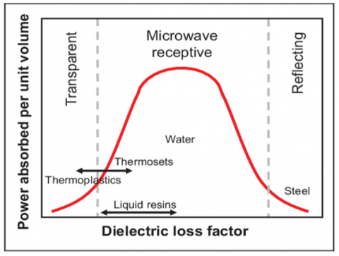
As for materials, yellow copper has been used in the manufacture of the external cavity, as it is characterized by excellent properties in electrical connection, which reduces electromagnetic energy loss and improves the efficiency of the sensor. The yellow copper also provides protection from external interference, which increases the sensitivity and accuracy of the sensor. In addition, Coupling Structures are combined with a diameter of 15 mm to ensure the insertion and exit of electromagnetic signals with high efficiency. The diagram demonstrates the connection between dielectric loss factor and energy absorption rate per unit volume in order to enhance understanding about designing cylindrical cavities for microwave applications. Fluid and thermoplastic substances transparent to microwave frequencies stand opposite to water and similar materials that show high microwave penetration levels thus requiring powerful coupling systems. Insulation purposes need materials with high dielectric loss since they reflect electromagnetic energy like steel does. The ongoing work enables the development of brass cylindrical cavities by selecting proper materials together with ideal dimensions for optimal electromagnetic wave coupling as well as supporting investigations into the effects of different geometric parameters illustrated in Figure 2 [20].
Figure 2. The relationship between the power absorbed per unit volume and the dielectric loss factor of different materials [21]
After preparing the sample and selecting the dimensions based on previous studies, the experimental setup was designed with a cylindrical cavity based on the diameters of the tubes under study. The diameters (4) cm were chosen for horizontal flow testing in the Ministry of Science and Technology / Department of Industrial Research and Development laboratory.
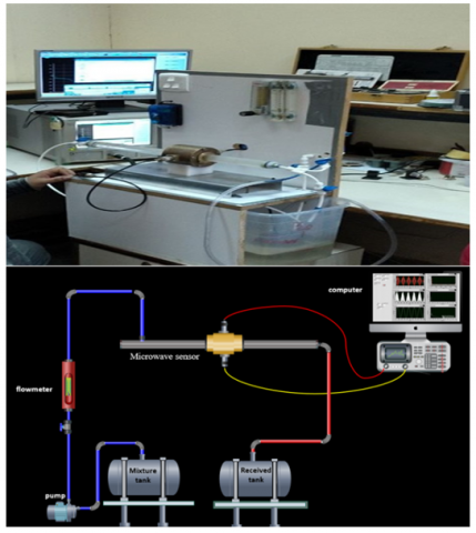
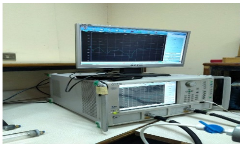
The sample preparation consists of a horizontal cylindrical cavity made of brass containing variable diameters according to the tube diameter used in the study. It also includes a pump to pump the mixture (Water and PEG) that controls the Water mechanism through a valve, as shown in Figure 3. Sample tubes are utilised to introduce substances into the cavity for examination. The cavity sensor apparatus is linked to an Agilent network analyser functioning within the 3-4 GHz range. The analyser device is linked to Port 1 (P1) and Port 2 (P2) by precision cables and appropriate adapters.
The microwave operates by reflecting electromagnetic waves perfectly through a polished copper cylinder. It measures the water content in a liquid mixture with different proportions of water by passing waves through a transparent acrylic tube. The idea lies in how to change the resonant frequencies according to the electrical properties of the materials. The cylindrical vacuum resonant body was designed from a copper alloy, and a lathe machine was used to carve the vacuum resonant body and also to produce the vacuum. Likewise, the cover's hole comes in different diameters, which align with the diameter of the tubing used for the flow as Figure 4.
Figure 3. (a) The experimental rig (b) Schematic diagram of the experimental
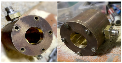
Figure 4. Fabricated cylindrical cavity resonator
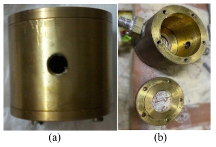
For the part, the cylinder is drilled from the top with a 4 cm hole to pass an acrylic rod, and from the side, it is drilled with a diameter of 10 cm on two opposite sides for mounting a Waveguide adapter with a dipole antenna as Figure 5.
Figure 5. Hole in fabricated cylindrical cavity resonator (a) Side view and (b) Top view
This experiment utilises three acrylic pipes of varying diameters (4cm) and a length of 50 cm. These pipes are interconnected through a manifold area for Water and PEG for different (mixture) supplies, and the opposite end empties into the mixing tank.
Electrical conductivity can vary greatly in brake fluids and water mixes. Increased water volume fractions are often associated with higher conductivity. The chemical formula for polyethene glycol, H-(OCH2CH2)n-OH, is typically used in commercially available braking fluid recipes. The reason behind the high electrical permittivity of the braking fluid, commonly represented as ε = 27 when n = 3, is its chemical makeup. The viscosity of the braking fluid is also strongly dependent on the shear rate due to its non-Newtonian fluid behaviour. In the range of 10 s-1 to 0.1 s-1 shear rate, its viscosity usually varies from 0.7 Ns/m2 to 1000 Ns/m2. Approximately 800 kg/m3 is the density of standard braking fluid made of polyethene glycol. However, Water has a constant viscosity of 1.0 Ns/m2, behaving like a Newtonian fluid. At room temperature of 25℃, it has a higher density of 1000 kg/m3 and a higher electrical permittivity of 78.5, respectively. These empirical data and basic chemical laboratory studies support this project's selection of microwave cavity resonator technology [22].
The complete tool setup for performance an illustration of the tests is shown in Figure 3. The tests were conducted using the VNA tool at the Ministry of Science and Technology / Department of Industrial Research and Development laboratory. The data was then shown on the VNA and the screen, as seen in Figure 6. The hollow can be filled with several substances, including Water, PEG, and a combination of Water and PEG.
The brake fluid (PEG) system with water yielded phase ratio readings at Mix.1, Mix.2, Mix.3, pure water and PEG, for illustrated in Table 1 utilising a benign and non-intrusive microwave cavity-based sensor that scans the entire sample. It was contingent upon the S22 measurements that estimate the extent to which microwave radiation infiltrates the combination.
Figure 6. Show data in VNA and screen
Table 1. Composition and types of water-PEG mixtures
|
No |
Sample Type |
Type of Mixture |
|
1 |
Water |
Pure water |
|
2 |
PEG |
Pure PEG |
|
4 |
Mix.1 |
70 % water with PEG |
|
5 |
Mix.2 |
50 % water with PEG |
|
6 |
Mix.3 |
30 % water with PEG |
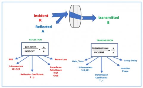
The reflection-to-incident ratio is denoted as A/R, whereas transmittance is defined as B/R, based on the receiver's measurements in the network device analyser, as illustrated in Figure 7 and Figure 8.
Figure 7. Mathematical illustration of waves
Figure 8. Comprehensive schematic of power wave patterns
The load, representing the typical impedance of the testing system, is indicated $Z_0$ [23].
SNR: Signal–to–Noise Ratio.
Return Loss, Impedance, Admittance: R+jX, G+jB
specific description of the incident power wave at any given port is:
$a=\frac{1}{2} \frac{\left(V+Z_0 I\right)}{\sqrt{\left|R\left\{Z_0\right\}\right|}}$ (3)
The wave of reflected power throughout any port can be characterized as:
$b=\frac{1}{2} \frac{\left(V+Z_0^* I\right)}{\sqrt{\left|R\left\{Z_0\right\}\right|}}$ (4)
The S-parameter matrix specifies the powers of the reflected and incident waves.
$b=\mathrm{S} a$ (5)
The elements of S are a $N \times N$ matrix.
Efficient power networks: Electrical power dissipation within the network does not lead to any reduction or loss [24].
$\mathrm{S}_{22}=\frac{{ Reflected }}{{ Incident }}=\left.\frac{b_2}{a_2}\right|_{a_{1=0}}$ (6)
A comprehensive flow diagram of power waves is presented. The load matches the characteristic impedance of the testing system. The variables of network analysis and signal processing are also incorporated.
$S_{22}$: Represents the reflection ratio of the reflected signal at $Z=0$.
$a$: Symbolizes the reflected signal from the incident signal at $Z=0$.
$b$: Represents the transmitted signal from the reflected signal at $Z=0$.
7.1 Characteristics of S-parameter
Reasons for developing S-parameters:
They are easily obtainable at high frequencies.
A vector network analyzer (VNA) can measure voltage-traveling waves.
Bypass or short connections are crucial, as failure may lead to device oscillation and potential self-destruction.
These measurements include gain, loss, reflection coefficients, and other parameters.
S-parameters from cascaded devices facilitate system performance evaluation.
S-parameter measurement files can be easily shared and integrated into the HFSS simulation package.
7.2 The relationship between S-parameters and the permittivity of a mixture
This study concentrates on the reflected S-parameters. Our investigations revealed that the resonant frequencies are distinctly pronounced and highly responsive to alterations within the 3-4 GHz region for the reflected S22 parameters. The gathered experimental data quantifies both the reflected and transmitted characteristics. The permittivity of the mixture can be inferred from the reflected S-parameter, S22, as determined in reference [25].
$S_{22}=\frac{\left(\frac{1}{R}-R\right)\left(e^{\gamma d}-e^{-\gamma d}\right)}{D}$ (7)
The ratio of characteristic impedance with and without the test material is shown as R. The diameter of the material sample being tested is denoted by d, D represents the denominator quantity, and γ signifies the propagation constant.
Where $\gamma$ and $R$ can be found depending on frequency and cut-off frequency as follows,
$R=\sqrt{\frac{1-\left(\frac{f_c}{f}\right)^2}{\varepsilon_{M R}^{\prime}-I \varepsilon_{M R}^{\prime}-\left(\frac{f_c}{f}\right)^2}}$ (8)
$\gamma=i \frac{\omega}{c} \sqrt{\varepsilon_{m r}^{\prime}-i \varepsilon_{m r}^{\prime \prime}-\left(\frac{f_c}{f}\right)^2}$ (9)
where, $f_c, \omega, \varepsilon_{m r}^{\prime}, \varepsilon_{m r}^{\prime \prime}$, i and c represent the cut-off frequency, angular frequency, real, imaginary parts of mixture relative permittivity, $\sqrt{-1}$ and light speed $\left(3 \times 10^8 \mathrm{~ms}^{-1}\right)$ respectively.
7.3 Mixture permittivity
The determination of water-PEG (brake fluid) permittivity remains essential for microwave sensing applications together with dielectric analysis requirements. Multiple mathematical models serve to determine effective permittivity measurements of these mixture types. The models have different applicable scenarios with distinct assumptions about their behavior. The following section provides an analysis of available models together with justification for choosing the optimal model for water-PEG systems for Table 2.
Table 2. Comparison of mathematical models for mixture permittivity calculation
|
Model |
β |
Advantages |
Limitations |
|
Power Law |
Variables |
Flexible; general framework |
Requires specific β for accurate results |
|
Looyenga Model |
1/3 |
Captures nonlinear interactions; suited for water-PEG |
May not apply to heterogeneous systems |
|
Lichtenecker Model |
0 |
Accurate for heterogeneous mixtures |
Less accurate for nonlinear systems |
|
Bertsch Model |
1/2 |
Balances simplicity and accuracy |
Limited to moderately nonlinear systems |
|
Sebrstein Model |
1 |
Simple and efficient |
Fails for nonlinear mixtures like water-PEG
|
The mixture's relative permittivity of water-PEG is determined using several mathematical formulae. A well-known approximation is the power law [26].
$\varepsilon_{\mathrm{r}, \mathrm{eff}}^\beta=\mathrm{f}_1 \varepsilon_{\mathrm{r}, \mathrm{w}}^\beta+\mathrm{f}_2 \varepsilon_{\mathrm{r}, \mathrm{EPG}}^\beta+\left(1-\mathrm{f}_1-\mathrm{f}_2\right) \varepsilon_{\mathrm{r}, \mathrm{g}}^\beta$ (10)
where, $\varepsilon_{\mathrm{reff}}$ represents the relative effective permittivity of the mixture. $\varepsilon_{\mathrm{r}, \mathrm{w}}, \varepsilon_{\mathrm{r}, \mathrm{EPG}} \& \varepsilon_{\mathrm{r}, \mathrm{g}}$ represent the relative permittivity of water, EPG, and gas, respectively. $\mathrm{f}_1$ represents the volume fraction of water, $f_2$ represents the volume fraction of PEG (brake fluid), and β is the power parameter, if applicable.
When $\beta=\frac{1}{3}$, the following equation will provide the Looyenga formula.
7.4 Looyenga model
The Looyenga usage in studying water-PEG mixtures is advantageous because the model incorporates nonlinear water-PEG molecule interactions that exist in homogeneous liquid-liquid systems.
$\begin{gathered}\varepsilon_{r, e f f}=\varepsilon_{r, w}+ {\left[3 f_2 \varepsilon_{r, w}^{\frac{2}{3}}\left(\varepsilon_{r, E P G}^{\frac{1}{3}}-\varepsilon_{r, w}^{\frac{1}{3}}\right)+3 f_2^{\frac{2}{2}} \varepsilon_{r, w}^{\frac{2}{3}}\left(\varepsilon_{r, E P G}^{\frac{1}{3}}-\varepsilon_{r, w}^{\frac{1}{3}}\right)^2\right]} \\ +\left[3 f_3 \varepsilon_{r, w}^{\frac{2}{3}}\left(\varepsilon_{r, a}^{\frac{1}{3}}-\varepsilon_{r, w}^{\frac{1}{3}}\right)++3 f_3^2 \varepsilon_{r, w}^{\frac{2}{3}}\left(\varepsilon_{r, a}^{\frac{1}{3}}-\varepsilon_{r, w}^{\frac{1}{3}}\right)^2\right.\end{gathered}$ (11)
To obtain a more diverse method for determining the effective refractive index of a mixture, please consult references [27].
7.5 Analysis of water permittivity
Relative permittivity is a mathematical notion consisting of two components: the real part, termed the dielectric constant, and the imaginary part, designated as the dielectric loss. It regulates the reflection of electromagnetic waves at any interface and the attenuation of wave energy within materials [28]. To ascertain the relative permittivity of a composite material, it is essential to know the permittivity of its constituent constituents. The permittivity of water is delineated.
$\varepsilon_{r, w}=\varepsilon_r^{\prime}-i \varepsilon_r^{\prime \prime}$ (12)
The dielectric constant, which is the real component, is defined as the stored energy originating from an electric field.
$\varepsilon_{\mathrm{r}}^{\prime}=\frac{\varepsilon_{\mathrm{s}}-\varepsilon_{\infty}}{1+\omega^2 \tau^2}+\varepsilon_{\infty}$ (13)
where, $\varepsilon_s$ and $\varepsilon_{\infty}$ denote static and infinite permittivity’s, respectively, while $\omega$ and $\tau$ signify angular frequency ($2 \pi f$) in radians per second and relaxation time in seconds, respectively.
The program is named High-Frequency Structure Simulator. Numerical techniques are employed for finite element analysis. The system's primary structure is segmented into discrete components with technical specifications. Tetrahedra serve as the finite elements in this study, with a mesh denoting their aggregation. Upon resolving the finite element fields, the interconnections among them are removed to satisfy Maxwell's equations at the element boundaries. This approach offers a comprehensive answer over the whole field. Upon determining the field solution, proceed to ascertain the S-matrix solution [29].
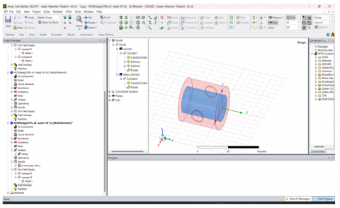
In this research, Ansys Twin Builder 2022 R1 was used as shown in Figure 9.
Figure 9. Depicts a physics model of a cylindrical cavity device utilizing the mixture in the HFSS software
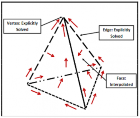
The HFSS adaptive solution procedure validates the accuracy of the results derived from the electromagnetic problem under investigation. Tetrahedral elements get processed in computational simulations by directly solving vertices and edges while performing face interpolations. This method plays a vital role since it maintains correct physics representation as well as efficient computation of results. [30, 31]. The method stands out as important for advanced research in fluid dynamics and heat transfer and structural analysis because it explicitly solves critical points while interpolating interpolation across faces between these points for precision and resource efficiency balance, as seen in Figure 10.
Figure 10. Finite elements for a tetrahedron tangential vector
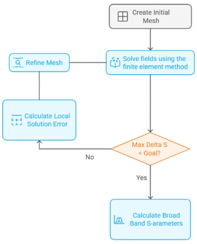
The main steps of the adaptive solution process for the procedural foundation begins by mesh generation that splits a geometric domain into virtual subdivisions before conducting numerical analysis. The finite element method (FEM) operates on the initial mesh configuration to generate physical results regarding quantity measurements. The local solution error gets evaluated by examining differences occurring between calculated results after this step. The computations run again once mesh refinement occurs when the error surpasses the set threshold value. The computational process will repeat until the remaining error reaches a level that is lower than the predefined target value. The system moves to broadband S-parameter calculation after reaching the targeted accuracy level to achieve complete evaluation of electromagnetic performance as shown Figure 11.
Figure 11. Flow diagram of the adaptive solution process
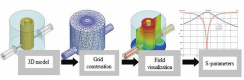
Figure 12. 3D model grid construction field S-parameters visualization in HFSS building
The process of simulating a three-dimensional model using HFSS software starts with designing a 3D model of the target device, as illustrated by Figure 12. The next step is to build a grid around the model, which is an essential step for accurate analysis of the electric and magnetic fields. After that, field visualization approaches are used to provide insights into the wave’s interaction with each of the elements in the model. The last step is the extraction of S-parameters, which is a very exact characterization of the electromagnetic wave behavior and hence the overall model output characteristics [29].
8.1 HFSS procedure
Creating and solving steps of specified HFSS simulation will be:
•Generate 3D structure: The initial step in the process involves creating a three-dimensional structure for further analysis.
•Solve: This step involves solving the problem or simulation following the structure generation.
•Apply boundaries and excitations: In this step, boundaries and excitations are defined and applied to the model.
•Post-process: After solving the simulation, post-processing is done to analyze and interpret the results.
•Solution setup: This step involves setting up the solution parameters before proceeding with the simulation.
•Results processing.
8.2 Two-phase problem simulation
In order to determine the resonant frequencies of various materials, including water and brake fluids, the Eigen-mode and Driven modal techniques are used. In this analysis we hope to assess the Electromagnetic Characteristics of the designed antenna which include the resonant frequencies and the Q-Factor. In Eigen-mode solution, the resonant frequencies are selected by considering five modes, at a minimum frequency step at each frequency of the range from 2GHz to 4GHz, and five passes are carried out for better results. Next, the Driven modal solution is performed with experimental tests conducted to accurately determine the number of modes, with ten passes completed at a maximum delta S-parameter of 0.01 at a frequency of 3GHz. Furthermore, an analysis of the frequency sweep is also performed in the range of 2-4 GHz with a step size of 0.0062422.
Table 3. Resonant frequency specification for the five eigen solution analyses
|
Frequency Range GHz |
Water |
EPG |
||
|
Resonant Frequency GHz |
Q-Factor |
Resonant Frequency |
Q-Factor |
|
|
1-2 5 modes |
2.01468 |
268.704 |
3.54364 |
25597.8 |
|
2-3 5 modes |
2.10813 |
277.428 |
3.54118 |
25676.2 |
|
3-4 5 modes |
3.2127 |
427.932 |
4.40389 |
36908.3 |
|
4-5 5 modes |
4.16007 |
528.59 |
4.40308 |
36959.7 |
|
5-6 5 modes |
5.05525 |
2765.75 |
5.12781 |
41009.4 |
This physical input includes values concerning relative permittivity and the conduction as bulk conductivities of the coupled materials. The results are demonstrated in a tabular form showing the resonant frequencies and quality factors for various materials at different frequencies where the data is then used to determine the highest resonant frequencies and quality factors Table 3 presents the results of this solution. Since the boundaries are symmetrical, the model was divided into two symmetrical sections so as to enable a quicker simulation of the model.
The research investigates water and brake fluid cavity materials because of their dielectric constant properties [32]. Different water volume fractions ranging for 0%, 30%, 50%, 70% and 100% were used for the modal analysis. Symmetrized boundary conditions were employed to improve computational performance in all three parts including the cylinder and ports together with the sample section. The simulation runtime decreased through a method which split the model into symmetrical sections and analyzed only one section because the accuracy of results remained unaffected. This method products efficient resource usage and accurate modeling of system properties alongside physical interactions.
8.3 Error estimation
In order to validate the simulation, it is necessary to compare the experimental results with the simulation results. This can be accomplished by calculating the percentage erro [33].
$\begin{aligned} & \% { Error } =\frac{ { Experimental\,\,Results }- { Sumulation\,\,Results }}{{ Experimetal\,\,Results }}\end{aligned}$ (14)
Since the exact amount is unknown, we divided it by the measured experimental value instead. Since the exact amount is unknown, divided it by the measured experimental value instead.
The detection capability of the microwave sensor relies on its ability to identify small variations in the dielectric properties of the tested material, which are directly correlated with its water content. The sensor's minimum detectable change in water content varies depending on the sensor frequency, in combination with calibration parameters linked to the material's electromagnetic properties.
The sensor exhibits a detection range of 0.1% to 0.5% in water content variation, influenced by system configuration and external environmental conditions. Its measurement accuracy is determined by the calibration technique and the stability of the measurement system, with an expected error range of +1% to -2%, applicable to most use cases.
For optimal sensor performance, well-controlled experimental conditions are essential, as noise, temperature fluctuations, and material inconsistencies can reduce sensitivity and resolution (refer to Table 4).
Table 4. Error and accuracy analysis for measured values
|
Error Percentage (%) |
Measured Value (%) |
Relative Error (RE) |
Accuracy (A) |
|
18% |
24.6% to 35.4% |
18% |
82% |
|
20% |
24% to 36% |
20% |
80% |
8.4 Comparison between experimental and theoretical results
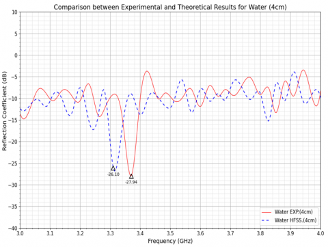
The comparative analysis of curves derived from various calculated and experimental results across differing frequencies ranging from 3 GHz to 4 GHz, as discussed in the earlier exposition, demonstrates a clear trend: the results are negative, suggesting that water does not reflect any electromagnetic energy and hence readily absorbs energy therein. This behavior can be environmentally supported in Figure 13 with events at −26.10 dB and −27.94 dB being statistically significant. Such points demonstrate that, there are changes in reflection coefficients when the MUT composition has been altered, and these values reduce significantly from their former values; hence changing interaction behaviors. Experimental and theoretical results present percentage errors between 18% to 20% because the system experiences complex interactions coupled with measurement uncertainties. Numerous factors which encompass material inaccuracy and measurement imprecision along with theoretical simplifications explain the observed variations between experimental and theoretical results. The theoretical model demonstrates accurate reproduction of essential physical effects based on the data from curve comparison analysis of the system.
Figure 13. Comparison between experimental and theoretical results for S22 of Mix.2 (4 cm)
Brief explanation of the need to involve the subject in the further discussion of the measurement of the water content in the brake fluid with the help of a microwave device. The investigation of properties of various fluids is deem necessary in many an aspect of engineering and sciences. In this case, a cylindrical microwave device was employed for the assessment of the water content in the brake fluid with a 4 cm diameter of acrylic tube inserted passing through it. Varying experiments were carried out using a solution of water with the proportions of 30%, 50%, and 70% and the goal of identifying the changes of the properties of the examined fluid.
Consequently, this work can be considered as making a further contribution to understanding the variations in material properties of the fluid, particularly where concentration of water is a major factor, along with thermal conductivity and viscosity of the fluid, which are deemed significant in the context of numerous applications in industry. From the results obtained from the experiments, it is possible to determine the impacts of water concentration on the fluid properties to design systems that enhance the proper-ties of the fluid. Our subsequent analysis will focus on the results produced by the experiments and discus the concentrations of water and their effects on the efficacy of density and viscosity measuring for fluids with similar physical characteristics.
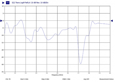
9.1 Results extracted from VNA measurements: Determining water content in peg (brake fluid)
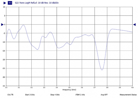
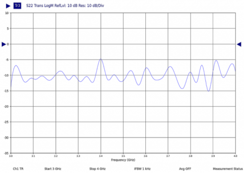
This study conducted VNA measurements to ascertain the water content of brake fluid (PEG). This investigation was conducted within a frequency range of 3 to 4 GHz, utilizing the S22 parameter to assess the reflection characteristics of the fluid. The study's conclusions indicated alterations in the observed signal level that signify fluctuations in water concentration within the fluid. The fluctuations are crucial for characterizing the dielectric constant of PEG, as its water content determines its electromagnetic response. Understanding the correlation between signal response and water content in the samples, we developed a method to quantify moisture concentration in stop fluids by the analysis of S22 data. This method enhances moisture detection accuracy and is beneficial in various fluid-based industrial processes where such information is crucial (refer to Figures 14-18).
Figure 14. Results extracted from VNA measurements pure water
Figure 15. Results extracted from VNA measurements Mix.1
Figure 16. Results extracted from VNA measurements Mix.2
Figure 17. Results extracted from VNA measurements Mix.2
Figure 18. Results extracted from VNA measurements PEG
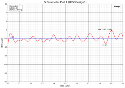
9.2 Simulation of electromagnetic properties of S22 parameter using HFSS: A study on PEG effects
S-parameter measurements, particularly S22, play a crucial role in evaluating system performance at high frequencies. This study investigates the behavior of S22 within the 3 GHz to 4 GHz frequency range, considering mixtures of water stoppers at 30%, 50%, and 70%, as well as pure water solvent and pure stopping fluid. The simulations were conducted using HFSS, a software well-suited for analyzing the electromagnetic properties of materials under various conditions.
The study of effect of water addition in the brake fluid (PEG) inside 4 cm diameter tube was a main topic for both electrical engineering and materials science. Experimental results reveal that the permittivity and conductivity of the resultant mixture changes considerably when introducing water, leading to significant alterations in reflection coefficients for frequencies between 3–4 GHz Such changes can be attributed to the intricate water and PEG interactions referred as a plasticizing agent, since it increases the ability of absorbing energy from mixture due to high carbon dioxide generation recently reported by the study [34]. But it is worth noting that increasing the water content in the brake fluid can slow down its effects of by degrading brake efficiency on systems used for various applications.
Characterization of properties but its physical property is changing when the water was adding, it can be seen in Figures 14-22. This behaviour is identified as one in which the reflection coefficient increases with water content, accompanied by a higher energy loss, the influence of permittivity is illustrated at different frequencies through which we can judge how it would become difficult to convey energy on account of water increasing its volume. The figures conductance versus water content shows the changing behaviour in response to hot components within a mixture.
Figure 19. Results of S-parameter (S22) study in the HFSS simulation for PEG flow with pure water
Figure 20. Results of S-parameter (S22) study in the HFSS simulation for PEG flow with 70% water
Figure 21. Results of S-parameter (S22) study in the HFSS simulation for PEG flow with 50% water
Figure 22. Results of S-parameter (S22) study in the HFSS simulation for PEG flow with 30% water
The net results of this analysis suggest that for water, the level of absorption is higher in comparison to others components (in a mixture), since energy reflected from port 2 has more losses. The ratio of moisture between the constituents is directly proportional to an increased auditory frequency loss coefficient enhancing water effectivity on overall performances. This highlights the need-to-know physical dynamics of individual particles to help design electronic systems [35]. Here it is extremely important to tweak up the water content if needed and be sure about balancing between having an effective brake fluid and inefficient [35].
This can help in understanding how the water as well as PEG affect the system for example by determining resonance ratios of a mixture components via information’s about their permittivity and conductivity. We use these results to identify the moisture amount in stopping fluid, thus assisting with offline endeavors like fabrication engineering and electronic system design.
9.3 Comparison between experimental and theoretical results for the reflection coefficient of water (4 cm)
The Curve Comparison with respect to the various calculated and experimental results of different frequencies from 3 GHz to 4 GHZ for water reflection coefficient. From the previous commentary, it is easily discernable that negative reflection coefficient values mean water absorbs electromagnetic energy but not in a reflecting manner. For example, it can be seen in the figures that at −26.10 and −27.94 dB there are critical points on a chart, these represent highlights how the variation of chemical elements transformation leads to changes its behavior as well through reflection coefficients significantly reduced.
In this case, it is possible to trust the program that was used for calculations which then showed their coincidence of experimental and theoretical results in determining percentage amount of water on the stopping fluid. This reliance is due to the precision of it leading all results converge and hence by using this program, we can confidently rely on its output for determining the water content in other mixtures. Hence, application of such computational tools can play a significant role for better understanding the material interactions with EM waves and their applications in different fields as shown Figure 23.
Figure 23. Comparison between experimental and theoretical results for the reflection coefficient of water (4 cm)
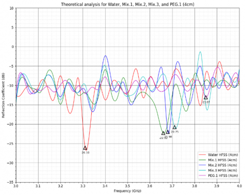
9.4 Analysing the reflection coefficient of mixtures theoretically at frequencies ranging from 3 to 4 (GHz)
The reflection coefficient for various combinations of water and different concentrations of PEG has been theoretically calculated within the 3–4 GHz frequency range, as shown in Figure 24. In the chart, the x-axis represents frequency (GHz), while the y-axis represents the reflection coefficient (dB). The color-coded lines indicate different materials: red for water, green for Mix.1, blue for Mix.2, purple for Mix.3, and black for PEG.
The negative reflection coefficient values are primarily due to energy absorption rather than reflection, significantly influencing the electrical properties of the materials. This effect is particularly evident in the reflectivity curve. Notably, the graph and system frequency response do not align as expected, mainly because material reflection coefficients vary significantly across different frequencies and chemical compositions, affecting their overall behavior.
This analysis is crucial for the design of electronic systems, as it helps evaluate the response of materials to electromagnetic waves. Key factors such as reflection properties, electrical conductivity, and specific energy absorption rates for each mixture can be assessed, allowing for the determination of optimal water content proportions in the development of advanced components.
Figure 24. Analysis of reflection coefficient for a series of mixtures at 3 to 4 GHz
Measurement Accuracy: The design of the cylindrical microwave sensor shows that the device has the potential of accurately determining the degree of water content in brake fluid hence improving the safety of performance in braking systems.
Impact of Chemical Composition: The results provide evidence of the variation of the reflection coefficient based on the variation of the chemical concentration of the brake fluid confirming the relevant effect upon the designing of sensors.
Reliability of Results: The reiteration of experimental results with theory strengthens the stability of microwave sensors as accurate instruments in measuring water in brake fluids.
Multiple Applications: This technology could be adopted in other related fields that may need measurement of water content in various fluids expanding its use in industries and medicine.
Efficiency Improvement: Microwave sensors are known to assist in enhancing the efficiency of braking systems through tracking of water content with a view of minimizing failure related risks.
Development of Measurement Tools: The results suggest potential for creating new ways of measuring via microwave technology and therefore, further creativity in sensor construction.
[1] Aqachmar, Z., Raoufi, M., El Gourari, A., Bouhal, T., Jenhi, M., Hajji, B., Barhdadi, A. (2022). Modelization and simulation of a low cost concentrated photovoltaic solar cell: Parametric and sensitivity study under MATLAB. Instrumentation Mesure Métrologie, 21(1): 1-6. https://doi.org/10.18280/i2m.210101
[2] Irawan, A.P., Fitriyana, D.F., Tezara, C., Siregar, J.P., Laksmidewi, D., et al. (2022). Overview of the important factors influencing the performance of eco-friendly brake pads. Polymers, 14(6): 1180. https://doi.org/10.3390/polym14061180
[3] Sethupathi, P.B., Chandradass, J., Saibalaji, M.A. (2021). Comparative study of disc brake pads sold in Indian market—Impact on safety and environmental aspects. Environmental Technology & Innovation, 21: 101245. https://doi.org/10.1016/j.eti.2020.101245
[4] Sunday, B., Usman, T., Mijinyawa, E.P., Ityokumbul, I.S. (2019). An overview of hydraulic brake fluid contamination. In Proceedings of the 15th iSTEAMS Research Nexus Conference, Abeokuta, Nigeria, pp. 47-56. https://doi.org/10.22624/AIMS/iSTEAMS-2019/V15N1P5
[5] Hunter, J.E., Cartier, S.S., Temple, D.J., Mason, R.C. (1998). Brake fluid vaporization as a contributing factor in motor vehicle collisions. SAE Transactions, 107: 867-885.
[6] Tseng, W.K., Chou, H.J. (2020). An alarm system for detecting moisture content in vehicle brake fluid with temperature compensation. International Journal of Mechanical Engineering, 7(12): 1-6. https://doi.org/10.14445/23488360/IJME-V7I12P101
[7] Kiani, S., Rezaei, P., Navaei, M. (2020). Dual-sensing and dual-frequency microwave SRR sensor for liquid samples permittivity detection. Measurement, 160: 107805. https://doi.org/10.1016/j.measurement.2020.107805
[8] Ebrahimi, A., Tovar-Lopez, F.J., Scott, J., Ghorbani, K. (2020). Differential microwave sensor for characterization of glycerol–water solutions. Sensors and Actuators B: Chemical, 321: 128561. https://doi.org/10.1016/j.snb.2020.128561
[9] Yang, Y., Xu, Y., Yuan, C., Wang, J., Wu, H., Zhang, T. (2021). Water cut measurement of oil–water two-phase flow in the resonant cavity sensor based on analytical field solution method. Measurement, 174: 109078. https://doi.org/10.1016/j.measurement.2021.109078
[10] Abdulsattar, R.K., Elwi, T.A., Abdul Hassain, Z.A. (2021). A new microwave sensor based on the moore fractal structure to detect water content in crude oil. Sensors, 21(21): 7143. https://doi.org/10.3390/s21217143
[11] Andria, G., Attivissimo, F., Di Nisio, A., Trotta, A., Camporeale, S.M., Pappalardi, P. (2019). Design of a microwave sensor for measurement of water in fuel contamination. Measurement, 136: 74-81. https://doi.org/10.1016/j.measurement.2018.12.076
[12] Teng, K.H., Shaw, A., Ateeq, M., Al-Shamma’a, A., et al. (2018). Design and implementation of a non-invasive real-time microwave sensor for assessing water hardness in heat exchangers. Journal of Electromagnetic Waves and Applications, 32(7): 797-811. https://doi.org/10.1080/09205071.2017.1406408
[13] Nyfors, E. (2005). Microwave semisectorial and other resonator sensors for measuring materials under flow. In Electromagnetic Aquametry: Electromagnetic Wave Interaction with Water and Moist Substances, Berlin, Heidelberg, pp. 217-241.
[14] Komarov, V., Wang, S., Tang, J. (2005). Permittivity and measurements. Encyclopedia of RF and Microwave Engineering. https://doi.org/10.1002/0471654507.eme308
[15] Oon, C.S., Ateeq, M., Shaw, A., Wylie, S., Al-Shamma’a, A., Kazi, S.N. (2016). Detection of the gas–liquid two-phase flow regimes using non-intrusive microwave cylindrical cavity sensor. Journal of ElEctromagnEtic WavEs and applications, 30(17): 2241-2255. https://doi.org/10.1080/09205071.2016.1244019
[16] Al-Kizwini, M.A., Wylie, S.R., Al-Khafaji, D.A., Al-Shamma’a, A.I. (2013). The monitoring of the two phase flow-annular flow type regime using microwave sensor technique. Measurement, 46(1): 45-51. https://doi.org/10.1016/j. Measurement.2012.05.012
[17] Pozar, D.M. (2021). Microwave Engineering: Theory and Techniques (4th ed.). John Wiley & Sons, pp. 174-190. https://www.wiley.com/en-us/Microwave+Engineering%2C+4th+Edition-p-9780470631553.
[18] Collin, R. (2001). Fundations for Microwave Engineering (2nd ed.). https://csva.s3.amazonaws.com/schools/839/Civil/738/Foundations%20for%20Microwave%20Engineering%20by%20Robert%20E.%20Collin.pdf.
[19] Scott, A.W. (2005). Understanding Microwaves. John Wiley & Sons Inc. https://books.google.iq/books/about/Understanding_Microwaves.html?id=LHJGAAAAYAAJ&redir_esc=y.
[20] Sheen, J. (2007). Microwave measurements of dielectric properties using a closed cylindrical cavity dielectric resonator. IEEE Transactions on Dielectrics and Electrical Insulation, 14(5): 1139-1144. https://doi.org/10.1109/TDEI.2007.4339473
[21] Thostenson, E.T., Chou, T.W. (1999). Microwave processing: Fundamentals and applications. Composites Part A: Applied Science and Manufacturing, 30(9): 1055-1071. https://doi.org/10.1016/S1359-835X(99)00020-2
[22] Eshgarf, H., Nadooshan, A.A., Raisi, A. (2022). An overview on properties and applications of magnetorheological fluids: Dampers, batteries, valves and brakes. Journal of Energy Storage, 50: 104648. https://doi.org/10.1016/j.est.2022.104648
[23] Agilent Technologies. Agilent network analyzer basics. https://anlage.umd.edu/Microwave%20Measurements%20for%20Personal%20Web%20Site/Agilent%20NWA%20Basics%205965-7917E.pdf.
[24] Baden-Fuller, A. J. (1990). Microwaves: An Introduction to Microwave Theory and Techniques (3rd ed.). Pergamon. https://www.amazon.com/Microwaves-Third-Introduction-Microwave-Techniques/dp/0080404936-Microwave-Theory-and-Techniques.
[25] Challa, R., Kajfez, D., Demir, V., Gladden, J., Elsherbeni, A. (2008). Permittivity measurement with a non-standard waveguide by using TRL calibration and fractional linear data. Progress in Electromagnetics Research B, 2: 1-13.
[26] Shivola, A.H. (1989). Self-consistency aspects of dielectric mixing theories. IEEE Transactions on Geoscience and Remote Sensing, 27(4): 403-415. https://doi.org/10.1109/36.29560
[27] Sihvola, A.H. (1999). Electromagnetic Mixing Formulas and Applications (No.47). IET.
[28] Meissner, T., Wentz, F.J. (2004). The complex dielectric constant of pure and sea water from microwave satellite observations. IEEE Transactions on Geoscience and remote Sensing, 42(9): 1836-1849. https://doi.org/10.1109/TGRS.2004.831888
[29] Ansoft. (2009). HFSS user guide (Version 11.1). Ansoft LLC. https://www.scribd.com/document/363943560/HFSS-User-Guide-11-11.
[30] Djordjevic, A.R., Biljié, R.M., Likar-Smiljanic, V.D., Sarkar, T.K. (2001). Wideband frequency-domain characterization of FR-4 and time-domain causality. IEEE Transactions on Electromagnetic Compatibility, 43(4): 662-667. https://doi.org/10.1109/15.974647
[31] Sun, D.K., Lee, J.F., Cendes, Z. (2001). Construction of nearly orthogonal Nedelec bases for rapid convergence with multilevel preconditioned solvers. SIAM Journal on Scientific Computing, 23(4): 1053-1076. https://doi.org/10.1137/S1064827500367531
[32] Clippers Controls Inc. Dielectric properties of materials. http://www.clippercontrols.com/pages/Dielectric-Constant-Values.html.
[33] Wrede, R., Spiegel, M.R. (2002). Theory and Problems of Advanced Calculus. McGraw-Hill.
[34] Moon, J.D., Webber, T.R., Brown, D.R., Richardson, P.M., et al. (2024). Nanoscale water–polymer interactions tune macroscopic diffusivity of water in aqueous poly (ethylene oxide) solutions. Chemical Science, 15(7): 2495-2508. https://doi.org/10.1039/D3SC05377F
[35] Marioni, N., Nordness, O., Zhang, Z., Sujanani, R., et al. (2024). Ion and water dynamics in the transition from dry to wet conditions in salt-doped PEG. ACS Macro Letters, 13(3): 341-347. https://doi.org/10.1021/acsmacrolett.4c00046