Ramesh Babu Padamata*![]() | Sri Krishna Atluri
| Sri Krishna Atluri![]()
© 2023 IIETA. This article is published by IIETA and is licensed under the CC BY 4.0 license (http://creativecommons.org/licenses/by/4.0/).
OPEN ACCESS
Agriculture is critical to human survival. Almost 70% of the population is involved in agriculture, either directly or indirectly. There are no technologies in the old system to identify diseases in diverse crops in an agricultural environment, which is why farmers are not interested in expanding their agricultural productivity all days. Crop diseases control the growth and production of their particular species; hence early detection is also essential. There have been many attempts to use Machine Learning (ML) methods for disease detection and classification in agriculture, but recent advances in a subset of ML called Deep Learning (DL) have given this field of study renewed hope for improved accuracy. The widespread spread of diseases in the tomato crop has an impact on both the quality and quantity of the crop. A rapid, dependable, and non-destructive way of diagnosing Tomato diseases early on may be useful for farmers. The approach employs two deep learning based algorithms, the AlexNet and the SegNet Model, with input including seven different color images of tomato leaves, six of which are afflicted and one of which is healthy. This algorithm is applicable for other plants like potato, corn diseases of bacterial, fungul infection leaves. Some examples of hyperparameters that have been investigated for their effect on classification accuracy and execution time are mini-batch size, weights, and bias learning rate.
weight learning rate, tomato disease detection, deep learning, SegNet Model, mini-batch size, deep learning and Bias learning rate
Identification of crop diseases using digital cameras or mobile photographs looks to be difficult. A number of plant diseases and crops have benefited from the current trend of utilising several machine learning algorithms for disease diagnosis. [1]. Additionally, the progression of deep Convolutional Neural Network (CNN) related designs has greatly improved classification accuracy [2]. AlexNet, produced by Krizhevsky et al. [3] and worn to succeed the ImageNet Large Scale Visual Recognition Challenge (ILSVR - 2010) by correctly classifying thousand item classes from 1.3 million training pictures, was an unfortunately timed success. In AlexNet, each of the convolution layers has its own dynamic receptive field. Some layers use batch normalisation and maxpooling, and there are also convolution layers and a Rectified Linear Unit named as ReLU included. As compared to common shallow or one-dimensional machine learning algorithms with sufficient regularisation methodologies [4], our stacking design achieved significantly superior results. In order to classify images of diseases, Mohanty et al. [5] employed a transfer learning approach, defined as "the process of leveraging pre-trained AlexNet for categorization of new categories of picture". It used 54,316 images to accurately categorise 25 unique diseases across 15 crop species. With 23 layers, GoogleNet is more complex than AlexNet and has an inception module developed with a network-in-network architecture. AlexNet and GoogleNet were used to categorize eight different tomato diseases by Rangarajan et al. [6]. When compared to previous machine learning methods, that are the Support Vector Machine (SVM) and the random forest, the performance of the deep architectures was shown to be significantly greater. Several deep learning models [7] that are including the Visual Geometry Group named as VGG net, Inception V4, DenseNet, and ResNet, were put to the test on the Plant Village dataset, which contains information on 14 different plant species and their susceptibility to disease. With a test accuracy of 99.75%, DenseNet produced the best outcomes. To classify 9 illnesses and 1 healthy tomato crop in the PlantVillage dataset, Durmus et al. [8] employed AlexNet and SqueezeNet. AlexNet achieved 95.65% accuracy whereas SqueezeNet achieved 94.30% accuracy with the same amount of processing resources. To classify tomato illnesses, Shiji et al. [9] utilised VGG16 to extract the features as of the fully connected layer and then apply those features [10-16] to SVM. When applied to a test set, the aforementioned model achieved 88% classification accuracy.
Using the publicly available Village picture dataset, this study classified six distinct tomato crop illnesses and a healthy class using two pre-trained deep learning models, AlexNet [17-25] and SegNet [25-30] Model. The AlexNet [31] model's architecture and operational flow diagram are explored in detail in Section 2. In section 3, we covered the SegNet Model architecture and a tiered explanation of the precise tuning of the network for illness classification, as well as the effect of the specified hyperparameters. Section five detailed the improvement in performance over time and compared AlexNet and SegNet [7] models. The summary and citations were supplied in section 6.
This section gives a succinct overview of the deep learning model's architecture, including hardware and software configurations.
2.1 Hardware and software system configuration
The performance of deep learning models is highly dependent on GPUs that have the Compute Unified Device Architecture (CUDA) cores activated. The research was conducted using a GIGABYTE Geforce GTX 1050 Ti 4GB gddr5 pci-e Graphic Card (GV-N105TD5-4GD) as well as 8GB of Random Access Memory (RAM). For the purposes of this investigation, the AlexNet and SegNet Models included in MAT LAB 2017b were utilised.
2.2 AlexNet model
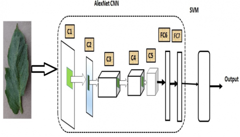
As can be seen in Figure 1, the pre-trained AlexNet model used in this analysis is primarily prepared up of five convolutional layers (conv layers) and three fully connected layers. In AlexNet, each of the convolution layers has its own dynamic receptive field. Some layers use batch normalisation and maxpooling, and there are also convolution layers and a Rectified Linear Unit named as ReLU included.
In the first starting convolution layer, an image with dimensions of 227×227×3 is processed via a filter with dimensions of 11x11x3. This filter represents the height, width, and depth of the input image. Specifically, the filter is work on a pixel by doing the dot product of the filtered matrix by the value of that pixel in the receptive fields of the input images. The 96 filters are applied the receptive fields in the first layer. At the end, the same no of activation maps are produced by the ReLU (Rectified Linear Unit) layer of the initial convolution layer. Using a same method, we performed convolutional operations on a second layer of convolutional with 256 filters with a dimension of 5×5×48, a third layer of convolutional with a count of 384 filters pixel dimension of 3×3×256, a fourth convolutional layer with a count of 384 filters of pixel dimension 3×3×192, and a fifth convolutional layer with a count of 256 filters of pixel dimension of 3×3×192, resulting in activation maps with distinct sets of neurons activated.
The resulted output of the preceding convolution layer is decreased in the dimension by fully connected layers, which do this by preserving the receptive field's maximum value. Forty thousand and nighty-six (4096) neurons are related to each other throughout layers six and seven. It has been shown that increasing network performance during testing is possible by using the dropout layer to randomly avoid the no. of connectional interfaces in a network for training [11]. The final completely linked layers have been fine-tuned to account for the entire complement of classes (7 in all, including the healthy category).
It was crucial that the model's main result was correct for the model to perform so well. GPUs, or Graphics Processing Units, make this possible during training while being very computationally costly. When it comes to convolutional neural networks, the hidden layers are involved of convolutional layers, pooling layers, fully connected layers, and normalising layers.
Using a filter to transform an image or signal is known as convolution. It's a method of sample-based discretization. The primary motivation is to reduce the high dimensionality of the input. Therefore, inferences may be drawn about the characteristics present in the discarded sub-regions.
The Convolutional Neural Network (CNN) Architecture is a multi-layered stack that utilises a differentiable function to convert an audio signal into a corresponding audio signal. That is to say, you may think of CNN architecture as just a particular stacking order for those components. Many distinct CNN designs have emerged over time as variants on common themes.
The most common amongst them are:
1. LeNet-5
2. AlexNet
3. ZFNet
4. GoogleNet
5. VGGNet
6. ResNet
There are five convolutional layers, three max-pooling layers, two normalisation layers, two fully connected layers, and last one softmax layer in AlexNet's architecture. Each layer of convolutional employs convolutional filters and the non-linear activation function called ReLU. For maximum pooling, utilise the layers designated as "pooling." Over sixty million parameters make up AlexNet. The winning model has been fine-tuned for a number of factors, including:
First, ReLU is an activation function. Second, it employed a technique known as a "Normalization layer," which is rarely used nowadays. Third, a batch sizes of 73, 173, 273, 373.
Fourth, SGD Momentum is an effective learning method. Fifth, extensive data enhancement by means of flipping, jittering, cropping, colour normalising, etc. Model assembly for optimal performance at last.
In the proposed paper we introduce the SegNet Model for image classification for better performance. Developed by a group of members in the University of Cambridge, the SegNet network is a free and open- source program for extracting the pixel-by-pixel boundaries of various objects in an image such as vehicles (cars, motorcycles), people, roads, and so on. There is no computational convolution or need for temporary storing of pixel blocks in SegNet networks. The SegNet Model architecture and a tiered explanation of the precise tuning of the network for illness classification, as well as the effect of the specified hyperparameters. These hyperparameters are used to improve the learning of the model, and their values are set before starting the learning process of the model. In Machine Learning/Deep Learning, a model is represented by its parameters. In contrast, a training process involves selecting the best/optimal hyperparameters that are used by learning algorithms to provide the best result. "Hyperparameters are defined as the parameters that are explicitly defined by the user to control the learning process."
In that they are taught from beginning to finish categorizing collections of pixels, they are analogous to more conventional neural networks. One distinctive feature of the SegNet network model is the presence of separate the encoding layers and decoding layers.
Figure 1. AlexNet architecture
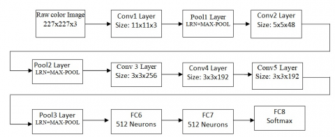
Figure 2. Flow diagram of AlextNet Convolutional Neural Network (CNN)
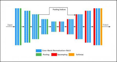
By constructing a symmetric encoder-decoder structure with the help of the semantic distribution of the full convolutional neural network, the network is able to carry out fully-fledged pixel-level image segmentation. This is accomplished by using the distribution of the full convolutional neural network. Downsampling is accomplished by the encoder through the utilization of pooling, while gradual restoration of the original image's spatial dimension and level of detail is accomplished by the decoder through the utilization of inverse convolution. When you're done with SegNet, you'll have a fully convolutional neural network. A coding network, a decoding network, and a pixel-level classification layer are the three basic components of the architecture. Low-resolution features can be attributed to the fact that the coding network's structure is identical to the layout of VGG16's 13 convolutional layers [14]. By reducing the encoding precision of the fully connected layer's output location, high-resolution feature maps are preserved. The low-resolution features are mapped into the entire input image-level resolution feature map, and the decoding network, which is responsible for pixel-level classification, essentially replaces the pooling layer in the coding network with the upsampling layer.
As a rule, the network may be divided in half. On the left, we find the encoding layer, which combines images into a single one and draws out the graph's high-dimensional data and attribute. The right side of the model is the decoding layer, which performs operations like deconvolution and upsampling. The Upsampling operation performs the image to its original size whereas deconvolution enables classification and feature regeneration. Finally, a segmentation map is generated using a softmax classifier as shown in Figure 2.
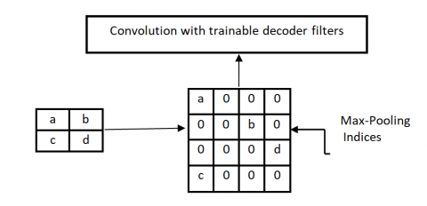
The term "pooling" refers to the process of collecting feature data from several locations within a defined region of an image. The SegNet network is downsampled using max pooling; the correct index position is saved during encoding, and the upsampled version is used during decoding. Pooling serves three main purposes, which are as follows: As a result of translational inconsistency, pooling abstracts regional characteristics without regard to position, thereby reducing the complexity and number of parameters required for optimization, and thereby increasing the perceptual region (as one pixel can correspond to an area in the original image).
The SegNet Model employs an upsampling strategy that uses a well crafted pooling index, which significantly lessens the amount of data that is lost as a result of the pooling process. To send the more information of the features since the layer jumping connection is used to carry the features of lower-layer. As a conclusion, the model is able to greatly increase the success rate of image segmentation.
Figure 3. A proposed SegNet Model
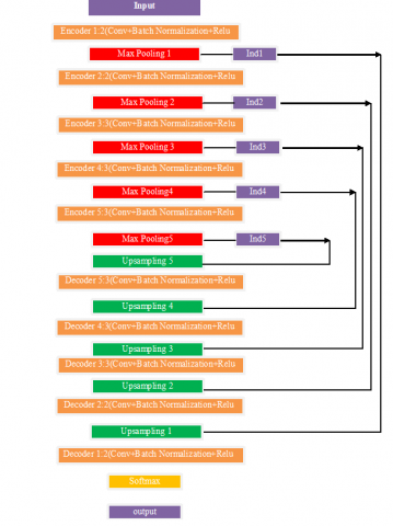
One component of the encoding layer that makes use of the SegNet Model network. Figure 3 depicts the subsample's division into five halves, each containing thirteen layers [14]. First and second parts have two 3 3 convolution layers and a 2 2 pooling layer, whereas third, fourth, and fifth sections have three 3 3 convolution layers and a 2 2 pooling layer. Activation functions trigger batch normalization after every convolution operation's output. The maximum pooling operation is used to extract picture features; the pooling layer stores its maximum index throughout each pooling operation (the location information of the maximum feature value, for example) and releases it during the upsampling process.
The decoding layer makes use of a mapping approach to convert the particular high-order, less resolution feature graph into a high resolution quality map. During the reverse of decoding is encoding process, the layer that keeps track of indices logs the highest value found in the pool. Figure 4 demonstrates how the decoding network accomplishes nonlinear upsampling on the picture using a pooled index in the biggest pooling layer, which does not need learning [15]. Figure 4 depicts the five-step decoding procedure that mirrors the five-step encoding process. The first and second parts are made up of a 2 2 deconvolution layer and two 3 3 convolutional layers, respectively. Following a 2 2 deconvolution layer and three 3 3 convolutions in the third, fourth, and fifth stages, a softmax classifier makes predictions for each pixel in the resultant feature picture in the sixth stage. The encoder has the potential to enhance edge characterization, decrease the number of network training parameters, and speed up the training process.
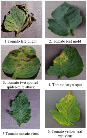
Experts in the fields of plant biology, epidemiology, and computer science are constantly developing new machine learning and deep learning strategies to combat a wide variety of plant diseases and improve crop yields. The researchers used the PlantVillage dataset [13] to get pictures of plants grown in a laboratory setting. Computer vision and deep learning have been used to develop very accurate systems for the autonomous detection of plant diseases. Combining pre-existing photos with well-known deep learning methods, image augmentation creates novel visuals in a wide range of settings. Tomatoes, potatoes, grapes, apples, maize, blueberries, raspberries, soybeans, squash, and strawberries are just a few of the 14 crops included in the over 50,000 images contained in the collection. Tomatoes will be our main produce. There are six main groups of tomato infections: 1) Late blight 2) Target Spot 3) Leaf Mold 4) Yellow Leaf Curl Virus 5) Mosaic virus 6) Spider mites: Two-spotted spider mite. In this proposed study, we use 6 different tomato leaf disease datasets in addition to 1 healthy tomato leaf as shown in Table 1, with a total of 16,000 pictures over the three datasets (10,000 for training, 7,000 for validation, and 500 for testing). Among the training set of 10,000 images, 1571 were assigned to the "healthy" group, while the remaining 15432 were assigned to each of the illness categories for tomatoes. While there are 700 photographs of each class in the validation set, there are 73, 173, 273, 373 images in the test set. For comparisons only we take the test sets for convenient and easy calculations.
We selected 73 images at random from each category in the training set before running the tests. Using the leftover training dataset, we divided the images evenly between classes and used it to create our project training dataset. When there were fewer than a thousand images available for any given category, we used data augmentation to create some more images.
The Python Augmentor package was used to accomplish the augmentation, which involved the rotation, flipping, cropping, and scaling of existing photographs to produce visually identical new ones. We picked the first 1000 images from each category in the training dataset when there were more than 1000 pictures in that category. On the validation set, we followed the identical steps and distributed 700 images to each category. This procedure is essential for CNN training to occur without discrimination toward a certain class. All the images are JPEGs with a 256x256 pixel resolution.
Table 1. The no. of tomato leaf images for healthy and unhealthy classes
|
Class |
Unhealthy |
Healthy |
||||
|
|
Fungi |
Bacteria |
Mold |
Virus |
Mite |
|
|
Sub Class |
Late blight-1910 |
Target spot-2127 |
Leaf Mold (1771) |
Yellow Leaf curl virus-5357 |
Two spotted spidermite-1676 |
Healthy-1591 |
|
|
|
|
Tomato Mosaic Virus-1000 |
|
|
|
Figure 4. The complete diagram of the detailed SegNet network
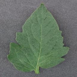
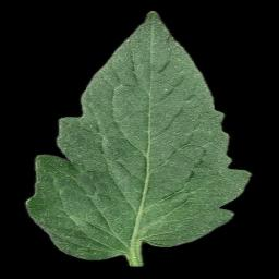
The Plant Village dataset [13] was used to collect tomato photos for six distinct illnesses as well as healthy tomato crop samples. To conduct this test, we segmented the dataset by setting the entire background pixels in the three different colour channels that are Red, Green, and Blue to 0 (as shown in Figure 5). There were 15432 segmented images in the dataset, including both those with diseases and those without diseases. To train the AlexNet model, we raised the input picture size to 227×227, while the SegNet Model used an even smaller image at 224×224. Increased noise in the original picture caused by signal oscillations is shown in Figure 6. The median filter averages out pictures by swapping out each pixel for its median. The main benefit of the median filter is that it maintains edges while reducing spikes.
As can be seen in Figure 7(a), the best method for dealing with random and unequal noise is to apply filters to the images. Salt and pepper noise is present in the majority of the images in the collection, according to the analysis. Research utilizing a median filter to decrease these sounds yielded the results shown in Figure 7(b). Both the SegNet Model's encoding layers and the Max pooling levels get the filtered picture as input.
Figure 5. Diagram of the unsampling process
Figure 6. Different diseases of tomato leaves dataset
Figure7(a). Original image
Figure7 (b). Filtered image
Using deep learning models that have already been trained, a technique called "transfer learning," is used to create new categories of objects. Initial analysis involved feeding the altered images into models of AlexNet and SegNet that had already been trained. To accommodate the models' training on the 1000 classes present in the village plant dataset, the last layer was swapped out for an output layer with the same amount of classes. There are seven categories total, with six different diseases and one category of healthy images. At last added a one softmax layer and one fully connected layer has been added to this design. The final three layers of both models were consequently revised as a consequence. The all-inclusive learning rate for both models is 0.0001. The last three layers of the classification network are fine-tuned with a bias learning rate of 20 and a weight learning rate of 10.
In other words, the learning rates for bias and weight are 20 and 10 times, respectively, faster than the total learning rate for the fully connecter layer 8, which is itself 10 times faster. It is a pre-trained network optimised for the classification of ImageNet datasets, therefore only the most basic of training parameters are used for the first few layers. Stochastic gradient descent with momentum is used to make the necessary adjustments to the weights, and it does so by averaging the gradients with an exponential weight. Minibatch size was 32 and the epoch number was set at 10. The minibatch size is shorthand for the lesser batches generated by partitioning the trained datasets into sections and updating the model's coefficients via gradient descent. The first step of developing weights for unequal selection is pretty straight forward. Adjusting Weights for Non Response The second step in weight development is about compensating for a unit or complete non-response. Making Addition Adjustments with Auxiliary Data. Checking Variability in Estimated Weights.
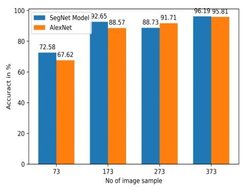
Using AlexNet and SegNet Models, we were able to acquire a classification accuracy of 97.49% and 97.23%, respectively, on a dataset of 13,264 images. In the next part of the research, the model performance was analysed by changing both the sample size and the hyperparameter. The performance and time required to run 10 epochs were examined after varying minibatch size, weight, and bias learning rate. Each class's accuracy was evaluated by having it classify the same amount of images. There were a total of 373 images in the tomato mosaic virus disease category. As a result, the AlexNet and SegNet Models can only take in as much as 373 image files per class as their input. Classification accuracy is shown in Figure 8; in each trial, 100 fewer images were used in the research.
Figure 8. Comparing the SegNet Model to Alex Net’s classification accuracy
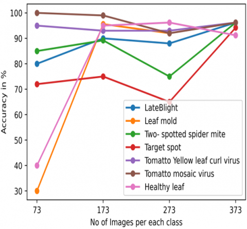
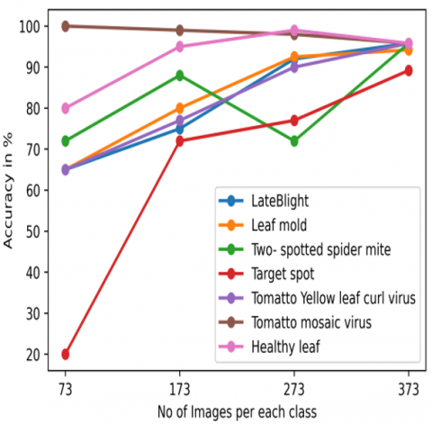
It proves the SegNet Model is superior to the AlexNet in almost every scenario. Both models improved when 373 images were included from each group. The SegNet Model achieved 96.19% accuracy in classification, whereas AlexNet only managed 95.81%, a slight decrease from the prior model. Figure 8 shows that as sample group reduces, prediction accuracy reduces. A comparison of the two architectures' performance on a dataset consisting of varied amounts of images for each class is shown in Figure 9. The AlexNet and SegNet Models can only take in as much as 373 image files per class as their input. In my model maximum data set must be 373 images.
Figure 9(a). SegNet Model classification accuracy for a class of images
Figure 9(b). Alex Net’s classification accuracy for a class of images
Both models achieved a maximum accuracy of 89.33% when classifying the target location from a set of 373 pictures. Figure 9(a) and 9(b) represents that the overall performance of the algorithms was negatively impacted by the class target point. In the instance of the SegNet Model, which consisted of 373 images for every class, healthy leaves and target spot disease had disturb on the performance of the SegNet Model.
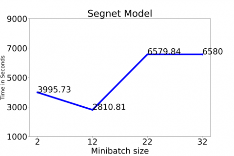
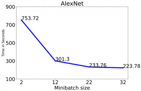
The following example examines the effect of varying a hyperparameter, minibatch size, on both classification precision and runtime. Comparison of the two models' runtimes was performed using 373 images and 10 epochs. Changing the minibatch size had a major impact on the execution time, as seen in Figures 10(a) and 10(b). The execution time rose as the minibatch size was increased in the SegNet Model, but it decreased in the AlexNet Model. It takes more time for the SegNet Model to process an image than it does for the AlexNet Model.
Figure 10(a). SegNet execution time analysis for different minibatch size
Figure 10(b). AlexNet execution time analysis for different minibatch size
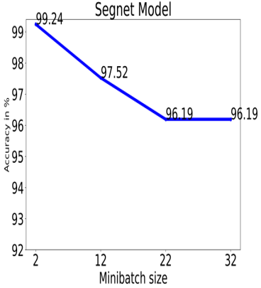
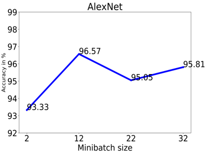
The SegNet Model obtains a maximum accuracy of 99.24% with a minibatch size of 2, whereas the AlexNet Model achieves a maximum accuracy of 96.51% with a size of minibatch is 12 (shown in Figures 11(a) and 11(b)). The target site consistently has low categorization accuracy relative to the other categories. The inability to tell the aforementioned class apart visually from the others may be to blame for its low accuracy. For the SegNet Model, if the minibatch size was more than 32, the algorithm could not be executed because of a memory allocation fault.
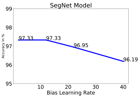
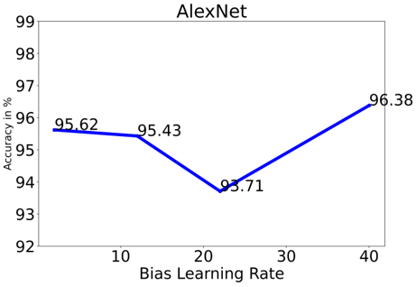
As shown in Figures 12(a) and 12(b), the subsequent portion of the experiment involved varying the weight and bias learning rate (b). If you use the SegNet Model and increase the bias and learning rate by a factor of 0 to 40 times the networks total learning rate, the accuracy of classification drops from 97.33% to 96.19%. But AlexNet's performance dropped until it reached a learning rate of 30, at which point it obtained a best classification accuracy of 96.38%. The SegNet Model accuracy was diminished by the rapid learning rate implemented in the final three layers.
Figure 11(a). SegNet classification accuracy analysis for different minibatch size
Figure 11(b). AlexNet classification accuracy analysis for different minibatch size
As a result, using the SegNet Model, the size of a minibatch is 2 and a learning rate that is just ten times the global learning rate yields the best results. However, AlexNet is effective since it is shallower, whereas the SegNet Model is computationally costly. Max accuracy of 96.38% is achieved with AlexNet using a size of a minibatch is 32 and a 40 is the used learning rate.
Images from the PlantVillage dataset were used for disease classification in the tomato crop, together with pre-trained deep learning architectures like AlexNet and the SegNet Model. In a test employing 13,269 images, the SegNet Model achieved a 97.29% accuracy in classification, while the AlexNet Model achieved a 97.49% accuracy. By adjusting the training set size, minibatch size, and weight and bias learning rates, we were able to evaluate the models' accuracy. The quality of the models was greatly affected by the number of images taken. For maximum precision, 373 images are used. Classification accuracy did not seem to decrease as a result of improvement the minibatch size in AlexNet, but it did decrease in the SegNet Model. When the minibatch size is less the SegNet Model is best. In a similar vein, Alex Net's accuracy dropped until it reached 30, and once the learning rate for weight and bias was fine-tuned. The accuracy of the SegNet Model improved with increasing weight and bias learning rates. The deep SegNet Model in terms of accuracy is also improved when compared to AlexNet and also less time to run, making it a more attractive option for use in production environments.
Figure 12(a). SegNet classification analysis using different weight and learning rate
Figure 12(b). AlexNet classification analysis using different weight and learning rate
The article describes a new method for identifying and categorizing different tomato plant leaf diseases based on their color, texture and shape. The study compares this method to existing models like AlexNet and SegNet, and found that the new model was more accurate at detecting diseases. The research focused on biotic diseases caused by fungal and bacterial pathogens such as blight, mold, and browns. In the future the researchers plan to expand the model to include abiotic diseases caused by nutrient deficiencies in the plant. They hope together more data on different plant diseases and use new technology to improve the accuracy of their model.
The 1st author conceived of the study, developed the methodology, software, validated the methodology, conducted the research, gathered the resources, selected the data, drafted the article, drafted, reviewed, and edited it, and created the visualisations. The second author has been in charge of project management and oversight.
[1] Barbedo, J.G.A.B. (2016) A review on the main challenges in automatic plant disease identification based on visible range images. Biosystems Engineering, 144: 52-60. https://doi.org/10.1016/j.biosystemseng.2016.01.017
[2] Liu, B., Zhang, Y., He, D., Li, Y. (2017). Identification of apple leaf diseases based on deep convolutional neural networks. Symmetry, 10(1): 11. https://doi.org/10.3390/sym10010011
[3] Krizhevsky, A., Sutskever, I., Hinton, G.E. (2015). Imagenet classification with deep convolutional neural network. Advances in Neural Information Processing Systems, pp. 1097-1105.
[4] Pasupa, K., Sunhem, W. (2016). A comparison between shallow and deep architecture classifiers on small dataset. In 2016 8th International Conference on Information Technology and Electrical Engineering (ICITEE), Yogyakarta, Indonesia, pp. 1-6, https://doi.org/10.1109/ICITEED.2016.7863293
[5] Mohanty, S.P., Hughes, D.P., Salathe, M. (2016). Using deep learning for image-based plant disease detection. Frontiers in Plant Science, 7: 1419. https://doi.org/10.3389/fpls.2016.01419
[6] Rangarajan, A.K., Purushothaman, R., Ramesh, A. (2018). Tomato crop disease classification using pre-trained deep learning algorithm. Procedia Computer Science, 133: 1040-1047. https://doi.org/10.1016/j.procs.2018.07.070
[7] Karnik, J., Suthar, A. (2023). Agricultural plant leaf disease detection using deep learning techniques. Proceedings of the 3rd International Conference on Communication & Information Processing (ICCIP). https://ssrn.com/abstract=3917556, accessed on Jan. 10, 2023.
[8] Durmuş, H., Gunes, E.O., Kirci, M. (2017). Disease detection on the leaves of the tomato plants by using deep learning. 2017 6th International Conference on Agro-Geoinformatics, VA, USA, pp. 1-5. https://doi.org/10.1109/Agro-Geoinformatics.2017.8047016
[9] Shijie, J., Peiyi, J., Siping, H., Haibo, L. (2017). Automatic detection of tomato disease and pests based on leaf images. Chinese Automation Congress, Jinan, China, pp. 3507-3510. https://doi.org/10.1109/CAC.2017.8243388
[10] Srivastava, N., Hinton, G., Krizhevsky, A, Sutskever, I., Salakhutdinov, R. (2015). Dropout: a simple way to prevent neural network from overfitting. Journal of Machine Learning Research, 15: 1929-1958.
[11] Hughes, D.P., Salathe, M. (2015). An open access repository of images on plant health to enable the development of mobile disease diagnostics. arXiv:1511.08060. https://doi.org/10.48550/arXiv.1511.08060
[12] Simonyan, K., Zisserman, A. (2014). Very deep convolutional networks for large-scale image recognition. arXiv:1409.1556. https://doi.org/10.48550/arXiv.1409.1556
[13] Badrinarayanan, V., Kendall, A., Cipolla, R. (2017). Segnet: A deep convolutional encoder-decoder architecture for image segmentation. IEEE. 39: 2481-2495. https://doi.org/10.1109/TPAMI.2016.2644615
[14] Long, J., Shelhamer, E., Darrell, T. (2015). Fully convolutional networks for semantic segmentation. Proceedings of the IEEE Conference on Computer Vision and Pattern Recognition, pp. 3431-3440.
[15] Brostow, G., Fauqueur, J., Cipolla, R. (2009). Semantic object classes in video: A high-definition ground truth database. PRL, 30(2): 88-97. https://doi.org/10.1016/j.patrec.2008.04.005
[16] Noh, H., Hong, S., Han, B. (2015). Learning deconvolution network for semantic segmentation. CoRR, arXiv:1505.04366. https://doi.org/10.48550/arXiv.1505.04366
[17] Liu, W., Rabinovich, A., Berg, A.C. (2015). Parsenet: Looking wider to see better. CoRR, arXiv:1506.04579. https://doi.org/10.48550/arXiv.1506.04579
[18] Chen, L., Papandreou, G., Kokkinos, I., Murphy, K., L. Yuille, A. (2014). Semantic image segmentation with deep convolutional nets and fully connected CRFs. IEEE, 40(4): 834-848. https://doi.org/10.1109/TPAMI.2017.2699184
[19] Hong, S., Noh, H., Han, B. (2015). Decoupled deep neural network for semisupervised semantic segmentation. arXiv:1506.04924. https://doi.org/10.48550/arXiv.1506.04924
[20] Hariharan, B., Arbelaez, P., Bourdev, L., Maji, S., Malik, J. (2011). Semantic´ contours from inverse detectors. Computer Vision (ICCV), Barcelona, Spain, pp. 991-998. https://doi.org/10.1109/ICCV.2011.6126343
[21] Arepalli, P.G., Akula, M., Kalli, R.S., Kolli, A., Popuri, V.P., Chalichama, S. (2022). Water quality prediction for salmon fish using gated recurrent unit (GRU) model. In 2022 Second International Conference on Computer Science, Engineering and Applications (ICCSEA), IEEE, pp. 1-5.
[22] Gu, Z., Cheng, J., Fu, H., Zhou, K., Hao, H., Zhao, Y., Zhang, T., Gao, S., Liu, J. (2019). CE-Net: Context encoder network for 2D medical image segmentation. arXiv: 1903.02740. https://doi.org/10.1109/TMI.2019.2903562
[23] Naqvi, R.A., Hussain, D., Loh, W.K. (2021). Artificial intelligence-based semantic segmentation of ocular regions for biometrics and healthcare applications. Computers, Materials & Continua, 66(1): 715-732. https://doi.org/10.32604/cmc.2020.013249
[24] Yamanakkanavar, N., Lee, B. (2020). Using a patch-wise M-Net convolutional neural network for tissue segmentation in brain MRI images. IEEE Access, 8: 120946-120958. https://doi.org/10.1109/ACCESS.2020.3006317
[25] Bhattacharya S., Mukherjee A., Phadikar S. (2020). A deep learning approach for the classification of rice leaf diseases. Intelligence Enabled Research. Advances in Intelligent Systems and Computing, Singapore, pp. 61-69. http://dx.doi.org/10.1007/978-981-15-2021-1_8
[26] Guo, Y., Zhang, J., Yin, C.X., Hu, X.N., Zou, Y., Xue, Z.P., Wang, W. (2020). Plant disease identification based on deep learning algorithm in smart farming. Discrete Dynamics in Nature and Society, 2020(2479172), 1-11. https://doi.org/10.1155/2020/2479172
[27] Faye, M., Chen, B.C., Sada, K.A. (2020). Plant disease detection with deep learning and feature extraction using plant village. Journal of Computer and Communications, 8(6): 10-22. http://dx.doi.org/10.4236/jcc.2020.86002
[28] Ayaluri, M.R., K, S.R., Konda, S.R., Chidirala, S.R. (2021). Efficient steganalysis using convolutional auto encoder network to ensure original image quality. PeerJ Computer Science, 7: e356. https://doi.org/10.7717/peerj-cs.356.,2021
[29] Abbas, A., Jain, S., Gour, M., Vankudothu, S. (2021). Tomato plant disease detection using transfer learning with C-GAN synthetic images. Computers and Electronics in Agriculture, 187, 106279. https://doi.org/10.1016/j.compag.2021.106279
[30] Karnik, J., Suthar, A. (2023). Agricultural plant leaf disease detection using deep learning techniques. Proceedings of the 3rd International Conference on Communication & Information Processing (ICCIP). https://ssrn.com/abstract=3917556, accessed on Jan. 10, 2023.
[31] Gopi, A.P., Gowthami, M., Srujana, T., Gnana Padmini, S., Durga Malleswari, M. (2022). Classification of Denial-of-service attacks in IoT networks using AlexNet. In Human-Centric Smart Computing: Proceedings of ICHCSC, Singapore, pp. 349-357.