Wahyudi Setiawan![]() | Moch. Andyka Saputra | Meidya Koeshardianto
| Moch. Andyka Saputra | Meidya Koeshardianto![]() | Riries Rulaningtyas*
| Riries Rulaningtyas*![]()
© 2024 The authors. This article is published by IIETA and is licensed under the CC BY 4.0 license (http://creativecommons.org/licenses/by/4.0/).
OPEN ACCESS
Seeds play an essential role in corn cultivation. Seed is one of the determining factors for plants to grow well. Corn seeds generally are diploid, with two chromosomes in one set. Besides diploid, there are haploid seeds that only have one chromosome. The haploid is only 0.1% of the total natural corn seed. Engineering technology development produced double haploid (DH). Corn seed yields can genetically improve plants. DH can shorten the period and improve breeding efficiency. In this article, we classify the image of corn seeds—public data from a rovile dataset with 1,230 haploid and 1,770 diploid images. The research steps included pre-processing, resizing, and undersampling the majority class for balanced data. Then, split 80% training and 20% testing data. The training data uses 5-fold cross-validation. Classification using a Convolutional Neural Network (CNN) with modified VGG architecture was made by adding two dropout layers 0.5 after the dense layer. The CNN architecture also uses transfer learning and fine-tuning techniques. Transfer learning improves performance, minimizes computing, and reduces training time. Fine tuning aims to taking a model that has been trained on a specific task and then piecing together the last few layers of that model to solve a new task. The model from the cross-validation results is then used for data testing. The test results show that the performance for accuracy, precision, recall, f1-score, and AUC is 96.83%, 95.9%, 98.87%, 97.36%, and 96.39%, respectively.
image classification, haploid-diploid, corn seed, VGG, transfer learning, fine-tuning, Convolutional Neural Network
Corn has many roles as food, feed, industrial raw material, and even cosmetic ingredients. Currently, the production of corn as feed is the most significant part of the utilization of corn products. The potential and demand that tends to increase is an opportunity and a challenge to increase production in quality and quantity [1, 2].
There are generally diploid and haploid seeds. Diploid seeds are present in most of the corn. Diploid seeds have two chromosomes in one set. In contrast, haploid seeds have only one chromosome in a group. Haploid seeds are substances that produce high-quality seeds. However, only 0.1% of haploid seeds are natural. Chromosomal engineering produces double haploid (DH) seeds. DH can increase corn's growth production and productivity [3, 4].
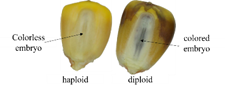
The manual selection of haploid seeds is strict because only very few diploid seeds are found, requiring a long process and a high error rate. Separation of seeds can be through differences in color in the embryo. Separation through color differences makes it possible to classify images. This research performs image classification for haploid and diploid seeds. It isn't easy to distinguish these two types of seeds by the naked eye, except with detailed observations. Figure 1 shows the visual difference between haploid and diploid seeds [5].
Haploid seeds have a colorless embryo, whereas diploid seeds tend to be dark brown.
Figure 1. Haploid and diploid corn seeds
An alternative for selecting haploid and diploid seeds is through computer vision (CV). This knowledge includes artificial intelligence, which trains computers to interpret and understand the visual world. CV involves image processing, machine learning, and deep learning. Image processing aims to improve images to make mining tasks easier. Meanwhile, machine learning and deep learning play a role in the feature extraction and image mining processes (classification, clustering, recognition, segmentation, and detection). The haploid and diploid seeds can be differentiated by classification mining.
The feature extraction process uses machine learning. The limitation of machine learning is determining features manually. Therefore, we use deep learning (DL). DL techniques extract simple to complex features from experimental datasets. In DL, feature extraction and classification only use one method. One that has widespread use is the Convolutional Neural Network (CNN) [5].
The benefits of classifying using computer vision compared to manual selection are:
Classification is essential in grouping an image based on class. Classification using the Convolutional Neural Network (CNN) with the popular transfer learning approach produces good performance. The transfer learning (TL) approach is used by utilizing a model that has been trained. TL provides faster training time than conventional methods. Generally, the model uses weights from the ImageNet dataset [6].
CNN has various architectural models. In previous studies, classification was done using the transfer learning pre-trained network from AlexNet, VGG, GoogleNet, and Resnet. Researchers reported that VGG-19 produced the highest accuracy at 94.22% [7]. In addition, other studies classify haploid and diploid using pre-trained networks such as Alexnet, GoogleNet, Resnet, and VGG. The classifier layer uses a decision tree, k-nearest Neighbor, and Support Vector Machine (SVM). Pre-trained network ResNet50 produces the highest accuracy of 91.4% [8].
In previous studies, the data between classes needed to be balanced. Therefore, there is an opportunity to improve performance. This study carried out the process of balancing the data with undersampling techniques.
Novelties in this research include:
Classification of haploid-diploid corn seed images has the following steps:
The complete steps of the proposed research are shown in Figure 2.
Figure 2. System proposed
2.1 Randomized undersampling
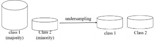
Randomized undersampling aims to balance data between classes. Undersampling is done by reducing the data in the majority class to the same as the minority class. The undersampling process is done by dropping randomized data on the majority class. The undersampling illustration is shown in Figure 3.
Figure 3. Technique undersampling
2.2 Visual Geometry Group (VGG)
VGG is one of the CNN series that won second place in the 2014 ImageNet Large Scale Visual Recognition Challenge (ILSVRC). However, VGG became the primary winner in the localization task. VGG is from the University of Oxford. Well-known VGG models are the VGG16 and VGG19. In this study, the VGG19 is used. The architecture comprises 19 layers, including 16 convolutional layers and three fully connected layers. Besides that, it has five max-pooling and one softmax layer. The number of parameters on VGG19 is over 144 million [9]. Therefore, this study uses modified VGG19 with more than 46 million parameters. The complete architecture of the modified VGG19 is shown in Table 1.
Modified VGG19 can be found in the classification layer; two dropout layers are 0.5 after the dense layer. Dropout performs random parameter deletion according to the input dropout value.
Table 1. Architecture of VGG19
|
No. |
Layer (type) |
Output Shape |
Param # |
|
1. |
input_1 (InputLayer) |
(None, 224, 224, 3) |
0 |
|
2. |
block1_conv1 (Conv2D) |
(None, 224, 224, 64) |
1792 |
|
3. |
block1_conv2 (Conv2D) |
(None, 224, 224, 64) |
36928 |
|
4. |
block1_pool (MaxPooling2D) |
(None, 112, 112, 64) |
0 |
|
5. |
block2_conv1 (Conv2D) |
(None, 112, 112, 128) |
73856 |
|
6. |
block2_conv2 (Conv2D) |
(None, 112, 112, 128) |
147584 |
|
7. |
block2_pool (MaxPooling2D) |
(None, 56, 56, 128) |
0 |
|
8. |
block3_conv1 (Conv2D) |
(None, 56, 56, 256) |
295168 |
|
9. |
block3_conv2 (Conv2D) |
(None, 56, 56, 256) |
590080 |
|
10. |
block3_conv3 (Conv2D) |
(None, 56, 56, 256) |
590080 |
|
11. |
block3_conv4 (Conv2D) |
(None, 56, 56, 256) |
590080 |
|
12. |
block3_pool (MaxPooling2D) |
(None, 28, 28, 256) |
0 |
|
13. |
block4_conv1 (Conv2D) |
(None, 28, 28, 512) |
1180160 |
|
14. |
block4_conv2 (Conv2D) |
(None, 28, 28, 512) |
2359808 |
|
15. |
block4_conv3 (Conv2D) |
(None, 28, 28, 512) |
2359808 |
|
16. |
block4_conv4 (Conv2D) |
(None, 28, 28, 512) |
2359808 |
|
17. |
block4_pool (MaxPooling2D) |
(None, 14, 14, 512) |
0 |
|
18. |
block5_conv1 (Conv2D) |
(None, 14, 14, 512) |
2359808 |
|
19. |
block5_conv2 (Conv2D) |
(None, 14, 14, 512) |
2359808 |
|
20. |
block5_conv3 (Conv2D) |
(None, 14, 14, 512) |
2359808 |
|
21. |
block5_conv4 (Conv2D) |
(None, 14, 14, 512) |
2359808 |
|
22. |
block5_pool (MaxPooling2D) |
(None, 7, 7, 512) |
0 |
|
23. |
to flatten |
(None, 25088) |
0 |
|
24. |
dense (Dense) |
(None, 1024) |
25691136 |
|
25. |
dropout (Dropout) |
(None, 1024) |
0 |
|
26. |
dense_1 (Dense) |
(None, 1024) |
1049600 |
|
27. |
dropout_1 (Dropout) |
(None, 1024) |
0 |
|
28. |
dense _2(Dense) |
(None, 2) |
2050 |
|
Total params: 46,767,170 Trainable params: 26,742,786 Non-trainable params: 20,024,384 |
|
||
Modified VGG19 has more than 46 million parameters, comprising 26 million trainable and 20 million non-trainable parameters. The difference between trainable and non-trainable parameters is updating the value of parameters. If trainable is updating, non-trainable is not updating during training.
The number of parameters in VGG19 is 144 million, so it takes more time to process them. Modified VGG19 adds dropout 0.5 twice. It can save resources by more than 66.67% (from 144 million to 46 million parameters).
2.3 Transfer learning and fine-tuning
Transfer learning (TL) aims to save computing resources. The system does not need to conduct training dataset experiments from the start. Transfer learning uses resources from previously trained pre-trained networks to new tasks. In this study, CNN uses the weights and biases of imagenet.
Meanwhile, fine-tuning aims to perform tuning according to the experimental dataset. Generally, fine-tuning is applied to the classification layer. If the results do not meet expectations, fine-tuning can be used for the final block convolutional layers that extract complex features.
Transfer learning uses an initial freeze, the first until the fourteenth convolution layer. Freeze layers aim to skip training on the basic features generated by the extraction feature layers. Furthermore, the fifteenth and sixteenth convolutional layers conduct training on the classification task of the new dataset. Figure 4 shows the steps of transfer learning [10, 11].
Figure 4. Transfer learning
Figure 4 shows an illustration of the transfer learning. Image data uses size 224. The convolutional layer block consists of the convolutional layer and max-pooling. The first up to the fourteenth convolutional layer is frozen and immediately retrieved from the imagenet weight.
The pre-trained network weights are not updated during training. One way to improve model performance is by training the weights of the VGG-19. The adjustments were made to some of the top layers rather than the entire VGG-19 layer.
The extraction feature layers learn simple and standard features in almost every image: the higher the layer, the more specific the features. Fine-tuning is done by unfreezing some of the classification layers. This technique makes refining the model more relevant for a particular task. The goal is to adapt special features to the new dataset. The model from the previous training is continued; this step can improve the model's performance.
Modification of VGG-19 was carried out in the classifier section with modifications according to fine-tuning carried out as a test scenario with unfreeze starting at layer 15. Fine-tuning aims to adapt the pre-trained model to new tasks—adaptation by training the corn seed image dataset. Fine-tuning is to retrain the model on new data. The classification layer section has a fully connected layer with activation of the rectified linear unit (relu) and softmax.
2.4 Cross-validation
When the training process requires proper validation, this research uses 5-fold cross-validation, which divides the training data into two parts: training and validation. Split into 80% training data and 20% validation data. At this stage, the aim is to get the model with the performance from five training and validation data variations. The model is saved for experiments using testing data [12, 13].
2.5 Performance measures
The confusion matrix is used in the model evaluation process as a solution to determine the performance of the CNN model. In the binary classification task, the confusion matrix includes four indices: True Positive (TP), True Negative (TN), False Positive (FP), and False Negative (FN) [14-16]. An illustration of the confusion matrix can be seen in Figure 5.
Figure 5. Confusion matrix
Performance measures include precision, recall, accuracy, f1-score, and Area Under Curve (AUC). The precision is determined by dividing the number of true positives by the total number of positive predictions made. The recall represents the accurate prediction of positive cases, indicating the total number of cases correctly identified. To determine the accuracy of a dataset, one must divide the total number of correct predictions by the overall dataset size. The f1-score is a measure of a model's accuracy, considering both precision and recall.
$A c c .=\frac{T P+T N}{T P+F P+T N+F N}$ (1)
$Prec. =\frac{T P}{T P+F P}$ (2)
$rec. =\frac{T P}{T P+F N}$ (3)
$f 1- score =\frac{2 \times T P}{2 \times(T P+F N+F P)}$ (4)
$A U C=\frac{1}{2}\left(\frac{T P}{T P+F N}+\frac{T N}{T N+F P}\right)$ (5)
If the accuracy, precision, recall, and f1-score can be obtained with the confusion matrix, the Receiver Operating Characteristic (ROC) curve shows the AUC value.
3.1 Test environment
This section describes the hardware and software testing environment used for experiments and test scenarios. The hardware consists of Google Colaboratory, Python 3, 12 GB RAM, Tesla T4 GPU, 78 GB Disk, Intel(R) Xeon(R) CPU @ 2.00GHz. Tensorflow Libraries 2.9.2, Keras 2.9.0. Numpy 1.21.6. Open CV 4.6.0.66, Seaborn 0.11.2, Scikit Learn 1.0.2, and Imblearn 0.8.1.
3.2 Experiment scenario
The test has four experiment scenarios. It aims to get the results. Comparison of imbalanced and balanced data and fine-tuning are the differentiating factors. Testing has four plans, including:
3.3 The dataset
Rovile public data has two classes, 1.230 haploid, and 1.770 diploid—total image data of 3,000. Split data training, validation, and testing are shown in Table 2.
Table 2. Split data
|
|
Imbalanced Data |
Balanced Data |
||
|
|
Haploid |
Diploid |
Haploid |
Diploid |
|
Training |
787 |
1133 |
787 |
787 |
|
Validation |
197 |
283 |
197 |
283 |
|
Testing |
246 |
354 |
246 |
354 |
|
Total |
1230 |
1770 |
1230 |
1338 |
In addition to balancing the data, it is necessary to initialize the hyperparameter values, learning rate 0.0001, epoch 64, and batch-size 32. Meanwhile, the Optimizer uses Adaptive Moment Estimation (Adam) [17]. The Adam optimizer combines two approaches: momentum and Adaptive sub-gradient from Root Means Square Propagation (RMSProp) [18] and Gradient Descent with Momentum (GDM) [19].
3.4 Result
3.4.1 Training with 5-fold cross-validation
The training data is split into training and validation data using 5-fold cross-validation. Tables 3 through 6 show the performance measures from the training results from the first until the fourth scenario.
Table 3. Result of the first scenario
|
fold |
Acc. |
Prec. |
Rec. |
f1-score |
AUC |
|
1 |
0.85 |
0.88 |
0.86 |
0.87 |
0.8462 |
|
2 |
0.86 |
0.88 |
0.88 |
0.88 |
0.8536 |
|
3 |
0.84 |
0.88 |
0.83 |
0.86 |
0.8365 |
|
4 |
0.88 |
0.92 |
0.88 |
0.90 |
0.8798 |
|
5 |
0.86 |
0.88 |
0.88 |
0.88 |
0.8519 |
Table 4. The result of the second scenario
|
fold |
Acc. |
Prec. |
Rec. |
f1-score |
AUC |
|
1 |
0.91 |
0.91 |
0.93 |
0.92 |
0.9063 |
|
2 |
0.97 |
0.99 |
0.95 |
0.97 |
0.9667 |
|
3 |
0.98 |
1.00 |
0.98 |
0.99 |
0.9833 |
|
4 |
0.99 |
1.00 |
0.98 |
0.99 |
0.9875 |
|
5 |
0.99 |
1.00 |
0.99 |
0.99 |
0.9917 |
Table 5. The result of the third scenario
|
fold |
Acc. |
Prec. |
Rec. |
f1-score |
AUC |
|
1 |
0.87 |
0.91 |
0.82 |
0.86 |
0.8706 |
|
2 |
0.88 |
0.92 |
0.84 |
0.88 |
0.8807 |
|
3 |
0.86 |
0.93 |
0.78 |
0.85 |
0.8629 |
|
4 |
0.85 |
0.87 |
0.83 |
0.85 |
0.8524 |
|
5 |
0.85 |
0.88 |
0.81 |
0.84 |
0.8499 |
Table 6. Result of the fourth scenario
|
fold |
Acc. |
Prec. |
Rec. |
f1-score |
AUC |
|
1 |
0.93 |
0.97 |
0.90 |
0.93 |
0.9340 |
|
2 |
0.96 |
0.99 |
0.93 |
0.96 |
0.9619 |
|
3 |
0.95 |
0.99 |
0.91 |
0.95 |
0.9518 |
|
4 |
0.97 |
0.98 |
0.95 |
0.97 |
0.9669 |
|
5 |
0.99 |
0.98 |
0.99 |
0.99 |
0.9873 |
Table 3 shows the results of the 5-fold cross-validation from scenarios 1 and 2. The training results in the first scenario (imagined data and without fine-tuning) show that fold-4 has the performance with an accuracy of 0.88, precision of 0.92, recall of 0.88, f1-score of 0.90, and AUC 0.8798.
Table 4 shows the result of the second scenario, using imbalanced data and fine-tuning to produce the performance on fold-5. The version achieved is accuracy 0.99, precision 1.00, recall 0.99, f1-score 0.99, and AUC 0.9917.
Tables 5 and 6 show the results of the third and fourth scenarios. After performing 5-fold cross-validation, the result is in the third scenario (balanced data without fine-tuning), fold-2—performance with accuracy 0.88, precision 0.92, recall 0.84, f1-score 0.88, and AUC 0.8807.
For fourth scenario (balanced data and fine-tuning). The training results show that the model is produced at fold-5. The performance consists of accuracy 0.99, precision 0.98, recall 0.99, f1-score 0.99, and AUC 0.9873.
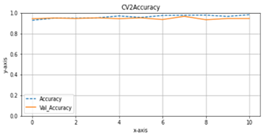
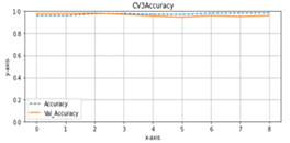
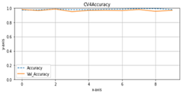
Accuracy and val_accuracy are metrics for evaluating model performance on classification tasks. Both calculate the ratio between the number of correct predictions and the total number of predictions made by the model, but there are differences in the data used. Accuracy is calculated on training data the model operates in the learning process, while val_accuracy is calculated on validation data not used in training. In model training, the main goal is to optimize the accuracy value of the training data so that the model can learn the patterns contained in the data. However, model performance is measured on training and validation data that the model has never seen before. If model performance on training data increases but performance on data validation decreases, this can indicate overfitting.
Val_accuracy that is lower than accuracy indicates that the model is learned from the training data and cannot generalize well to new data. Generalization is the ability of a model to produce accurate predictions on data that has never been seen before. Figure 6 shows that the accuracy and val_accuracy during the model training process can be generalized well to data that has never been seen before. The test results with the model are obtained in scenario 2. The model produced in scenario 2 is in fold-5.
(a)
(b)
(c)
(d)
(e)
Figure 6. Graphics of accuracy and validation accuracy in the second scenario. (a) until (e) is fold-1 until fold-5 (x-axis=epoch, y-axis=accuracy)
3.4.2 Time of training
This section describes the time needed to carry out the training process. Figure 7 shows the time required to train each fold of the second scenario.
Figure 7. The training time of the second scenario (in sec.)
Model training takes time, using Google Colaboratory Pro, the training time for the second experiment can be seen in Figure 7. Each fold that is trained requires a different training time from one another. One reason for the difference in training time is that the model training uses early stopping. It makes the model automatically stop according to the command given. They are making the amount of training for each model different. In the first test experiment, the time needed is around 150 to 400 seconds.
3.4.3 Receiver Operating Characteristic (ROC)
Figure 8. ROC result of the second scenario
The ROC Curve is a graph that evaluates the performance of a classification model in distinguishing between positive and negative classes. The ROC Curve line that is further away from the diagonal line indicates better model performance. The AUC value is the area under the ROC curve and provides a numerical value for model performance; the more significant the AUC value, the better the model performance [20-22]. Figure 8 shows the ROC with the AUC value in the second scenario.
ROC compares the true positive rate and false positive rate. The second scenario gained AUC 0.9917 in fold-5, as discussed in Table 4.
3.5 Testing experiment
The model from each scenario is used for experiments with testing data because there is no guarantee that the model from a system is optimal for testing in different methods. The testing data is 20%, excluding training and validation data.
When training a model, the dataset will usually be divided into three parts: training, validation, and testing data. The purpose of testing data is to test the model's performance on data the model has never seen before. In the model training process, we use the training data to teach the model how to recognize patterns and learn the relationship between features and labels. However, a model that is too adapted to the training data can cause overfitting. Therefore, we need validation data to evaluate model performance on data that has never been seen before and avoid overfitting.
After we have succeeded in selecting the model using validation data, we need to test the model's performance on testing data that the model has never seen before. It is essential to ensure that the model is optimal for training and validation data and generally usable for data that has never been seen before. Testing data can provide a more accurate evaluation of model performance and measure how well the model can be used in real situations. It helps to ensure that the model not only remembers the patterns present in the training data but also generalizes and performs well on data it has never seen before. Table 7 presents the results of the model performance from each experiment conducted on the testing data. The fourth test experiment gave the model performance results.
Table 7. The model testing results for each scenario
|
Scenario |
Acc. |
Prec. |
Rec. |
f1-score |
AUC |
|
1 |
0.918 |
0.896 |
0.975 |
0.934 |
0.906 |
|
2 |
0.952 |
0.931 |
0.992 |
0.960 |
0.943 |
|
3 |
0.907 |
0.907 |
0.938 |
0.922 |
0.899 |
|
4 |
0.968 |
0.959 |
0.989 |
0.974 |
0.964 |
After completing the training and validation process, the model is used to predict the testing data. The confusion matrix is used to measure model performance by comparing the number of correct and incorrect predictions made by the classifier in the model's testing set, as shown in Table 7. Because there are only two classes, haploid and diploid, in this study, the positive class has been determined as haploid, and the negative class has been selected as diploid. Among the samples labeled as haploid in the dataset is the TP data predicted by the haploid algorithm, which is haploid. What the algorithm predicts to be diploid but haploid is called FP. Among the samples labeled as diploid in the data set, so-called TNs are indicated by the algorithm as diploid. The algorithm also predicted data as haploid, but the truth is diploid is called FN. Table 8 shows the confusion matrix from the 20% testing results.
Table 8. Confusion matrix of all scenarios
|
Scenario 1 |
Scenario 2 |
Scenario 3 |
Scenario 4 |
||||
|
206a |
40b |
220a |
26b |
212a |
34b |
231a |
15b |
|
9c |
345d |
3c |
351d |
22c |
332d |
4c |
350d |
aTP; bFP; cFN; dTN
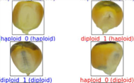
Figure 9. Sample of right and wrong recognition
The testing data is classified using the model obtained from the previous learning process. Scenario 4 gets the testing results. The results show an accuracy of 0.968, a precision of 0.959, a recall of 0.989, an f1-score of 0.974, and an AUC of 0.964. Figure 9 shows an example of an image successfully recognized correctly (text: blue) and incorrectly (text: red).
Table 8 shows that of the four test scenarios, haploid seeds have a higher FP value than diploid seeds. The difference between haploid and diploid seeds lies in the embryo's color and the endosperm at the top of the seeds. The embryo tends to be colorless in haploid seeds, and the endosperm is paler. On the other hand, diploid seeds have a more apparent dark brown color in the embryo and endosperm. Experiments show that there are more classification errors in haploid seeds.
This study used transfer learning and fine-tuning approaches to the modified VGG-19 model for classifying haploid and diploid corn seed images. It modified VGG-19 by adding twice dropout 0.5 after the dense layer. The transfer learning approach provides an advantage in applying a previously trained model to new data. Four test scenarios are carried out: unbalanced data without fine-tuning, unbalanced data with fine-tuning, balanced data without fine-tuning, and flat data with fine-tuning. The undersampling technique is used to balance between haploid and diploid data. Data balancing gives the result that with proportional data, it can minimize prediction errors from classes that have less data.
This study shows that the VGG-19 model can be used effectively for image classification of corn seeds. With balanced data and the application of fine-tuning, it has got the performance. The results show accuracy, precision, recall, f1-score, and AUC are 96.83%, 95.9%, 98.87%, 97.36%, and 96.39%.
This research has limitations, including that the resulting performance can still be improved. Next, the experiment can use multiclass for other types of corn seeds. Tuning can also be done to determine the influence of each CNN hyperparameter (learning rate, epoch, batch size)
This research can be used as an alternative to support the classification of haploid and diploid corn seeds. The system can be implemented automatically to recognize the data entered for further development directly.
This research funded by Penelitian Mandiri - National Collaborative Research - University of Trunojoyo Madura 2023.
[1] Berman, J., Zorrilla-López, U., Farré, G., Zhu, C., Sandmann, G., Twyman, R.M.,Christou, P. (2015). Nutritionally important carotenoids as consumer products. Phytochemistry Reviews, 14(5): 727-743 https://doi.org/10.1007/s11101-014-9373-1
[2] Panikkai, S., Nurmalina, R., Mulatsih, S., Purwati, H. (2017). Analisis ketersediaan jagung nasional menuju swasembada dengan pendekatan model dinamik. Inform. Pertan., 26(1): 41.
[3] Chaikam, V., Molenaar, W., Melchinger, A.E., Boddupalli, P.M. (2019). Doubled haploid technology for line development in maize: Technical advances and prospects. Theoretical and Applied Genetics, 132(12): 3227-3243. https://doi.org/10.1007/s00122-019-03433-x
[4] Turgut, İ. (2019). Production of double haploid plants using in vivo haploid techniques in corn. Journal of Agricultural Sciences, 25(1): 62-69. https://doi.org/10.15832/ankutbd.539000
[5] Altuntaş, Y., Kocamaz, A.F., Cömert, Z., Cengiz, R., Esmeray, M. (2018). Identification of haploid maize seeds using gray level co-occurrence matrix and machine learning techniques. In 2018 International Conference on Artificial Intelligence and Data Processing (IDAP), pp. 1-5. https://doi.org/10.1109/IDAP.2018.8620740
[6] Liao, W., Wang, X., An, D., Wei, Y. (2019). Hyperspectral imaging technology and transfer learning utilized in haploid maize seeds identification. In 2019 International Conference on High Performance Big Data and Intelligent Systems (HPBD&IS), pp.157-162. https://doi.org/10.1109/HPBDIS.2019.8735457
[7] Altuntaş, Y., Cömert, Z., Kocamaz, A.F. (2019). Identification of haploid and diploid maize seeds using convolutional neural networks and a transfer learning approach. Computers and Electronics in Agriculture, 163(40): 104874. https://doi.org/10.1016/j.compag.2019.104874
[8] Dönmez, E. (2020). Classification of haploid and diploid maize seeds based on pre-trained convolutional neural networks. Celal Bayar University Journal of Science, 16(3): 323-331. https://doi.org/10.18466/cbayarfbe.742889
[9] Simonyan, K., Zisserman, A. (2014). Very deep convolutional networks for large-scale image recognition. arXiv preprint arXiv:1409.1556. 1-14, https://doi.org/10.48550/arXiv.1409.1556
[10] Kim, Y.G., Kim, S., Cho, C.E., Song, I.H., Lee, H.J., Ahn, S., Kim, N. (2020). Effectiveness of transfer learning for enhancing tumor classification with a convolutional neural network on frozen sections. Scientific Reports, 10(1): 21899. https://doi.org/10.1038/s41598-020-78129-0
[11] Marlow, R., Kuriyakose, S., Mesaros, N., Han, H.H., Tomlinson, R., Faust, S.N., Finn, A. (2018). A phase III, open-label, randomised multicentre study to evaluate the immunogenicity and safety of a booster dose of two different reduced antigen diphtheria-tetanus-acellular pertussis-polio vaccines, when co-administered with measles-mumps-rubella vaccine in 3 and 4-year-old healthy children in the UK. Vaccine, 36(17): 2300-2306. https://doi.org/10.1016/j.vaccine.2018.03.021
[12] Arlot, S., Lerasle, M. (2012). Choice of V for V-fold cross-validation in least-squares density estimation. The Journal of Machine Learning Research, 17: 1-50. https://doi.org/10.48550/arXiv.1210.5830
[13] Anguita, D., Ghelardoni, L., Ghio, A., Oneto, L., Ridella, S. (2012). The'K'in K-fold Cross Validation. In ESANN pp. 441-446.
[14] Luque, A., Carrasco, A., Martín, A., de Las Heras, A. (2019). The impact of class imbalance in classification performance metrics based on the binary confusion matrix. Pattern Recognition, 91: 216-231. https://doi.org/10.1016/j.patcog.2019.02.023
[15] Belavkin, R., Pardalos, P., Principe, J. (2022). Value of information in the binary case and confusion matrix. In Physical Sciences Forum, 5(1): 8.
[16] Ruuska, S., Hämäläinen, W., Kajava, S., Mughal, M., Matilainen, P., Mononen, J. (2018). Evaluation of the confusion matrix method in the validation of an automated system for measuring feeding behaviour of cattle. Behavioural processes, 148: 56-62. https://doi.org/10.1016/j.beproc.2018.01.004
[17] Kingma, D.P., Ba, J. (2014). Adam: A method for stochastic optimization. arXiv preprint arXiv:1412.6980. in ICLR, 2015: 1-15. https://doi.org/10.48550/arXiv.1412.6980
[18] Hinton, G., Srivastava, N., Swersky, K. (2012). Lecture 6a overview of mini–batch gradient descent. Coursera Lecture slides.
[19] Ruder, S. (2016). An overview of gradient descent optimization algorithms. arXiv preprint arXiv:1609.04747. 1-14. https://doi.org/10.48550/arXiv.1609.04747
[20] Muschelli III, J. (2020). ROC and AUC with a binary predictor: A potentially misleading metric. Journal of classification, 37(3): 696-670. https://doi.org/10.1007/s00357-019-09345-1
[21] Huang, J., Ling, C.X. (2005). Using AUC and accuracy in evaluating learning algorithms. IEEE Transactions on knowledge and Data Engineering, 17(3): 299-310. https://doi.org/10.1109/TKDE.2005.50
[22] Narkhede, S. (2018). Understanding auc-roc curve. Towards data science, 26(1): 220-227.