Djedidi Imene* | Naimi Djemai | Salhi Ahmed | Bouhanik Anes
© 2022 IIETA. This article is published by IIETA and is licensed under the CC BY 4.0 license (http://creativecommons.org/licenses/by/4.0/).
OPEN ACCESS
This paper presents a novel and efficient optimization approach based on the Artificial Ecosystem Optimization (AEO) algorithm to solve the problem of finding optimal location and sizing of Distributed Generation (DGs) in radial distribution systems. The objective is to satisfy a fluctuating demand in a constant and instantaneous way while respecting the requirements of power loss reduction, operating cost minimization and voltage profile improvement within the equality and inequality constraints. The robustness of the proposed technique in terms of solution quality and convergence characteristics is evaluated using the IEEE-33 bus radial distribution network test system. The simulation results are compared with those of other methods recently used in the literature for the same test system. The experimental outcomes show that the proposed AEO approach is comparatively able to achieve a higher quality solution within a timeliness of computation.
Distributed Generation (DG), power loss, voltage profile, AEO, active network management, power distribution network
Nowadays, the integration of DGs is a key step in the active network management process for economic, ecological and political reasons [1]. The active management process permits, in particular, to decrease power plant capacity, increase the use of distribution networks, reinforce system security and minimize both operational costs and CO2 emission rates.
However, several challenges constrain the effective DGs integration. Among these challenges, the location and size of DG in the grid constitute a major integration issue. In fact, DG is located closer to the consumer and requires less transmission and distribution network services [2].
Also, experience shows that such integration affects the power flows in the grid. DGs are mainly based on renewable energies, local combined heat and power (CHP) plants and the use of wastes. For economic and geographical reasons, many of these sustainable energy sources are integrated into the distribution networks rather than transmission grids. The generation is then distributed within the system and not centralized.
But this integration leads to the inversion of the power flows and the distribution network becomes an active system where voltages, real (P) and reactive (Q) power flows are defined by the production as well as the loads and not a passive component feeding loads in a unidirectional power flow. The change in the behavior of the grid caused by DGs incorporation leads to important technical and economic consequences for the power system.
These are manifested by the increase in system losses, the disruption of voltage performance and consequently the increase in operational cost. Therefore, effective network connection involves the search for the optimal DGs location and size to address the above problems. Achieving this objective is an optimization problem for which many approaches have been proposed in order to provide solutions using appropriate methods. Mathematical methods include, among others, Newton Raphson load flow dedicated initially to the transmission networks are not adapted to the radial distribution network to which the DGs are connected and consequently do not provide accurate results [ 3]. Backward forward sweep is the most appropriate method for load flow analysis of radial distribution network [4].
Different metaheuristic methods are proposed to solve the DGs integration problem for optimal location and size such as the Whale Optimization Algorithm (WOA) [5], the Invasive Weed Optimization Algorithm (IWO) [6], the Artificial Bee Colony algorithm (ABC) [7], and the Dragonfly optimization Algorithm (DA) [8], multiple objective particle swarm optimization algorithm (MOPSO) [9]. The hybrid approach, which combines analytical and metaheuristic tools to deal with DGs optimal location and sizing problem, is suggested in Ref. [10].
Accordingly, this paper applies an efficient optimization approach based on the Artificial Ecosystem Optimization (AEO) [11] to solve the problem of optimal DGs location and sizing in radial distribution network.
The objective is to evaluate the convergence capabilities and the respect of the equality and inequality constraints of the AEO algorithm through various simulations.
These are performed on IEEE-33 bus test system by creating two different situations according to the type of integrated DG. Type 1 DG that injects only real power P to the system and Type 2 DG that injects both real P and reactive power Q [12]. The obtained results are compared to those of previous methods. The rest part of this paper is outlined as follows: Section II describes the mathematical model of the DG integration problem. Section III details the procedures of the AEO algorithm. Section IV provides simulation results. Finally, the main conclusions are given in Section V.
DGs integration problem is to minimize the active power losses in the system while satisfying several constraints associated to the power balance, voltage limits and operational cost. The complexity of the problem depends on the nature of the objective function and the type of the considered constraints. The optimal placement and sizing of DG in distribution network is determined from the solution of load flow equations using backward forward sweep technique within the AEO optimization framework (section 3). The objective function is defined as follows:
$\min f=\min T P_{L O S S}=\min \sum_{i=1}^{n_{b r}} P_{L O S S_{i}}$ (1)
where, $P_{L O S s_{i}}$ is power loss in $i$-th branch, $n_{b r}$ is the number of branches, $T P_{\text {LOSS }}$ is total real power loss.
$P_{L O S S_{i}}=R_{i} \cdot\left|I_{i}\right|^{2}$ (2)
where, Ri is the resistance of i-th branch in the network, Ii is the current magnitude of i-th branch.
The problem is to minimize system power losses while respecting the following constraints:
2.1 Equality constraints
Equality constraints are given by the power flow equations as follows:
$P_{\text {substation }}+\sum P_{D G}=P_{\text {load }}+\sum P_{\text {LOSS }}$ (3)
$Q_{\text {substation }}+\sum Q_{D G}=Q_{\text {load }}+\sum Q_{L O S S}$ (4)
2.2 Inequality constraints
The inequality constraints are defined as follows:
2.2.1 Bus voltage limits
$V_{\min } \leq\left|V_{i}\right| \leq V_{\max }; \quad i=1,2, \ldots, n_{\text {bus }}$ (5)
where, $V_{\min }=0.95(p u)$, and $V_{\max }=1.05(p u)$.
2.2.2 Branch current
$I_{i} \leq I_{\text {imax }}; \quad i=1,2, \ldots, n_{b r}$ (6)
where, $I_{i}$ is the current magnitude of i-th branch, $I_{i \max }$ is the maximum permitted current of i-th branch.
2.2.3 Size of DG
$P_{D G}^{\min } \leq\left|P_{D G i}\right| \leq P_{D G}^{\max }$; (7)
$Q_{D G}^{\min } \leq\left|Q_{D G i}\right| \leq Q_{D G}^{\max }$ (8)
2.2.4 Position of DG
$2 \leq D G_{b u s} \leq n_{b u s}$ (9)
where, $n_{\text {bus }}$ is the number of buses, $D G_{b u s}$ is the bus number of the DG installation, $V_{i}$ the bus voltage.
2.3 Operational costs
Operational costs are calculated using the following equations [5, 8]:
$C_{T P_{L O S S}}=T P_{L O S S} \times\left(K_{P}+K_{e}+L_{S f} \times 8760\right) \$$ (10)
$C_{D G}=\sum K_{D G_{P}} \times P_{D G}+\sum K_{D G_{q}} \times Q_{D G}$ (11)
$T O C=C_{T P_{L \Omega S S}}+C_{D G}$ (12)
where, $K_{P}$ is annual demand cost of power loss $(\$ / \mathrm{kW}), K_{e}$ is the annual cost of energy loss $(\$ / \mathrm{kWh}) ; L_{s f}$ is the loss factor expressed as:
$L_{s f}=K \times L_{f}+(1-K) \times L_{f}^{2}$ (13)
where,
$K=0.2, \quad L_{f}=0.47, \quad K_{P}=57.6923 \$ / K W$,
$K_{e}=0.0096153 \$ / K W h K_{D G_{P}}=5 \$ / K W$,
$K_{D G_{Q}}=0.2211 \$ / K V a r$.
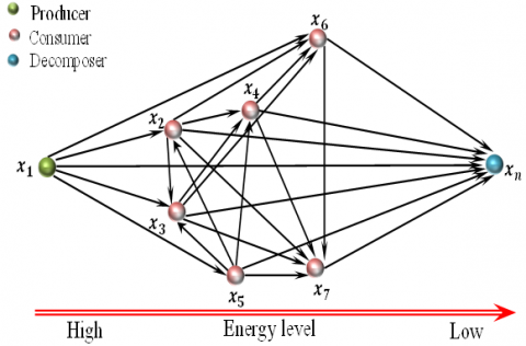
AEO algorithm is created by Zhao et al. [11] in 2019. According to the study [11] the AEO algorithm uses three different operators including production, consumption and decomposition. By analogy with living beings’ natural behaviors within the terrestrial ecosystem. The fundamental utility of these operators is to improve the optimum search process. This process is fully detailed in Ref. [11]. This section focuses on the mathematical basis supporting this tool. Figure 1 shows an AEO ecosystem according to which all individuals are ranked in decreasing sense of their fitness function, such that highest fitness value corresponds to highest energy level.
Figure 1. AEO ecosystem adapted from [11]
The mathematical equations that support the AEO model are given below [11]:
$x_{1}(t+1)=(1-a) x_{n}(t)+a x_{\text {rand }}(t)$ (14)
$a=\left(1-\frac{t}{T}\right) r_{1}$ (15)
$x_{\text {rand }}=\boldsymbol{r}(U-L)+L$ (16)
$C=\frac{1}{2} \frac{V_{1}}{\left|V_{2}\right|}$ (17)
$V_{1} \sim N(0,1), V_{2} \sim N(0,1)$ (18)
where, N(0,1) is a normal distribution with mean=0 and standard deviation = 1.
If the consumer is randomly selected as herbivore, it will eat only producers. The following equation describes this behavior:
$x_{i}(t+1)=x_{i}(t)+C \cdot\left(x_{i}(t)-x_{1}(t+1)\right), i \in[2, \ldots, n]$ (19)
If the consumer is selected as a carnivore, it will eat only the consumers with the higher energy level (lower fitness value). The equation modeling the consumption behavior of a carnivore is as follows:
$\left\{\begin{array}{c}x_{i}(t+1)=x_{i}(t)+C \cdot\left(x_{i}(t)-x_{j}(t)\right), i \in[2, \ldots, n] \\ j=\operatorname{randi}([2 i-1])\end{array}\right.$ (20)
When the consumer is chosen as an omnivore, the consumer has the ability to hunt other consumers with higher energy levels and/or producers. The consumption behavior of an omnivore can be mathematically formulated as follows:
$x_{i}(t+1)=x_{i}(t)+C \cdot\left(r_{2} \cdot\left(x_{i}(t)-x_{1}(t+1)\right)\right)+\left(1-r_{2}\right)\left(x_{i}(t)-x_{j}(t)\right), i \in[3, \ldots, n] j=\operatorname{randi}([2 i-1])$ (21)
$x_{i}(t+1)=x_{n}(t)+D \cdot\left(e \cdot x_{n}(t)-h \cdot x_{i}(t)\right), i=1, \ldots, n$ (22)
$D=3 u, \quad u \sim N(0,1)$ (23)
$e=r_{3} \cdot \operatorname{randi}\left(\left[\begin{array}{ll}1 & 2\end{array}\right]\right)-1,$ (24)
$h=2 \cdot r_{3}-1,$ (25)
where, a is linear weighting coefficient, $r$ is random vector from the interval $[0,1], r_{1}, r_{2}$ and $r_{3}$ are random numbers in $[0,1], L$ is search space lower limit, $U$ is search space upper limit, $N(0,1)$ is a normal distribution, $C$ and $D$ are consumption and decomposition factors, respectively.
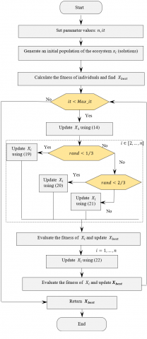
AEO initiates the optimization by generating a random population. For each iteration, the position of the first individual (producer) is updated based on (14), while other individuals in the population will update their positions according to (19), (20), and (21) regarding the type of the consumer except if the individual obtains a higher fitness value, then the position of such individual will be updated based on (22). The updating process will continue until the AEO reaches the end criterion. Finally, the optimal solution will be introduced. The overall process of the AEO is represented in Figure 2.
Figure 2. The AEO algorithm steps
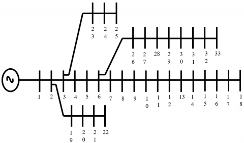
The IEEE-33 bus test system presented in Figure 3 is used to evaluate the AEO robustness. Its characteristics are listed in Table 1 [13]:
Table 1. IEEE-33 bus characteristics
|
Characteristics |
Values |
Units |
|
$n_{\text {bus }}$ |
33 |
[bus] |
|
$\mathrm{n}_{\mathrm{br}}$ |
32 |
[branch] |
|
$\mathrm{P}_{\text {load }}$ |
3.72 |
[MW] |
|
$Q_{\text {load }}$ |
2.30 |
[MVar] |
|
$\mathrm{V}_{\text {substat }}$ |
12.66 |
[KV] |
Figure 3. IEEE-33 bus test system [11]
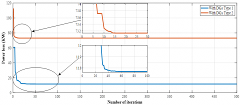
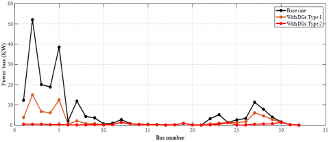
The results reported in Table 2, clearly show how losses decrease from 210.99 KW (base values) to 73.13 KW for DG type 1 integration and decrease to 11.76 KW for DG type 2 installation, minimum voltage values increase and operational costs reduce. These important outcomes are achieved during the first thirty iterations as illustrated in Figure 4.
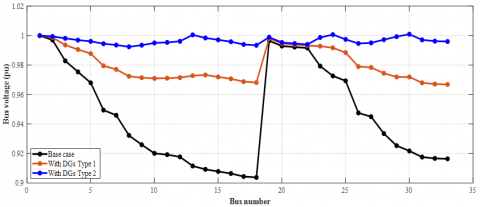
This notable decrease in losses enhanced in Figure 6 is accompanied by an improvement in the voltage profile highlighted in Figure 5.
AEO results are compared to those found with WOA, IWO ALO, and ABC methods as shown in Tables 3 and 4 for DG type 1 and DG type 2, respectively. AEO results are much better.
Figure 4. AEO convergence characteristics
Figure 5. Voltage profile of IEEE-33 bus system
Figure 6. Power Loss at every branch of IEEE-33 bus test system
Table 2. Summary of the obtained results
|
|
Uncompensated |
Compensated |
||||
|
Type 1 |
Type 2 |
|||||
|
bus |
$P_{D G}(K W)$ |
bus |
$P_{D G}(K W)$ |
$Q_{D G}(K V a r)$ |
||
|
DG Optimal location and size |
- |
14 |
755.7328 |
13 |
798.54 |
371.9419 |
|
30 |
1031.13 |
30 |
1039.2820 |
1008.2937 |
||
|
24 |
961.1931 |
24 |
1106.6686 |
504.5372 |
||
|
Total size of DG |
|
|
2748.05 |
|
2944.4907 |
1884.7728 |
|
Total $P_{L O S S}$ (KW) |
210.99 |
73.13 |
11.76 |
|||
|
Total $Q_{\text {LOSS }}$ (Kvar) |
143.13 |
50.78 |
9.8 |
|||
|
% Reduction in $P_{L O S S}$ |
- |
65.33 |
94.42 |
|||
|
% Reduction in $Q_{\text {LOSS }}$ |
- |
64.52 |
93.15 |
|||
|
Minimum voltage (pu) |
0.9038 |
0.9668 |
0.9924 |
|||
|
Operational costs (\$/year) |
512532.9979 |
191388.3115 |
43687.6397 |
|||
|
Net savings (\$/year) |
- |
321144.6864 |
468845.3582 |
|||
|
% Savings |
- |
62.65 |
91.47 |
|||
Table 3. DGs Type1: comparison results
|
Methods |
DG |
Power Loss (KW) |
% reduction in Power Loss |
Total Operational Cost (\$/year) |
Net savings (\$/year) |
% savings |
|
|
Size (KW) |
Bus |
||||||
|
WOA [5] |
1072.83 |
30 |
73.75 |
65.05 |
192664.151 |
319868.84 |
62.40 |
|
772.488 |
25 |
||||||
|
856.678 |
13 |
||||||
|
IWO [6] |
624.7 |
14 |
90.69 |
57.02 |
229232.973 |
283300.02 |
55.27 |
|
104.9 |
18 |
||||||
|
1056 |
32 |
||||||
|
ABC [7] |
1750 |
6 |
79.25 |
61.13 |
208014.8212 |
304518.1767 |
59.41 |
|
570 |
15 |
||||||
|
780 |
25 |
||||||
|
ALO [14] |
1500 |
32 |
75.26 |
65.01 |
195322.2769 |
317210.72 |
61.89 |
|
750 |
5 |
||||||
|
250 |
18 |
||||||
|
AEO |
755.7328 |
14 |
73.13 |
65.33 |
191388.3115 |
321144.6864 |
62.65 |
|
1031.13 |
30 |
||||||
|
961.1931 |
24 |
||||||
Table 4. DGs Type 2: comparison results
|
Method |
DG Size and location |
Power Loss (KW) |
% reduction in Power Loss |
Total Operational Cost (\$/year) |
Net savings (\$/year) |
% savings |
||
|
$P_{D G}(K W)$ |
$Q_{D G}($ KVar $)$ |
Bus |
||||||
|
WOA [5] |
1171.38 |
602.811 |
24 |
16.28 |
92.28 |
55023.42 |
457509.57 |
89.26 |
|
881.88 |
644.027 |
13 |
||||||
|
953.62 |
750 |
30 |
||||||
|
IWO [6] |
1098 |
766.26 |
6 |
22.29 |
89.43 |
69424.41 |
443108.58 |
86.45 |
|
1098 |
766.26 |
30 |
||||||
|
768 |
535.96 |
14 |
||||||
|
ABC [7] |
1014 |
628.21 |
12 |
15.91 |
92.45 |
55790.81 |
456742.18 |
89.11 |
|
960 |
594.76 |
25 |
||||||
|
1363 |
844.43 |
30 |
||||||
|
AEO |
798.54 |
371.9419 |
13 |
11.76 |
94.42 |
43687.6397 |
468845.3679 |
91.47 |
|
1039.282 |
1008.2937 |
30 |
||||||
|
1106.4907 |
504.5372 |
24 |
||||||
In this paper, AEO is applied to search DGs optimal location and sizing in radial distribution network, with main objective to minimize power losses and operating cost. This method is tasted on IEEE-33 bus test system. Depending on the nature of the injected power, two different situations are simulated.
The first consists on injecting only real power (Type 1), the obtained results clearly show how the values of the objective function (active power losses) and total operational cost decrease from 210.99 KW and 512532.9979 (\$/year) to 73.13 KW and 191388.3115 (\$/year) respectively, also the voltage profile has been improved from 0.9038 pu to 0.9698 pu.
In the second situation both real and reactive power are injected (Type 2), the obtained results show that the values of the objective function (active power losses) and total operational cost decrease from 210.99 KW and 512532.9979 (\$/year) to 11.76 KW and 43687.6397 (\$/year) respectively and it should be noted that the voltage profile has been dramatically increased from 0.9038 pu to 0.9924 pu.
The obtained results are compared with those of WOA, IWO, ABC and ALO methods to validate the efficiency of the AEO method. It’s concluded that the AEO algorithm, in comparison with other recent algorithms from the literature, provides the best optimum in terms of power loss, voltage profile, total operational cost and convergence capability.
[1] Jenkins, N., Ekanayak, Strbac, G. (2010). Distributed Generation. The Institution of Engineering and Technology, London, United Kingdom. https://doi.org/10.1049/PBRN001E
[2] Sivanagaraju, S., Satyanarayana, S. (2012). Electric power transmission and distribution. Dorling Kindersley Pvt. Ltd, India.
[3] Bayliss, C., Hardy, B. (2007). Transmission and Distribution Electrical Engineering. Elsevier Ltd.
[4] Bompard, E., Carpaneto, E., Chicco, G., Napoli, R. (2000). Convergence of the backward/forward sweep method for the load-flow analysis of radial distribution systems. International Journal of Electrical Power and Energy Systems, 22(7): 521-530. https://doi.org/10.1016/s0142-0615(00)00009-0
[5] Prakash, D.B., Lakshminarayana, C. (2018). Multiple DG placements in radial distribution system for multi objectives using Whale Optimization Algorithm. Alexandria Engineering Journal, 57(4): 2797-2806. https://doi.org/10.1016/j.aej.2017.11.003
[6] Rama Prabha, D., Jayabarathi, T. (2016). Optimal placement and sizing of multiple distributed generating units in distribution networks by invasive weed optimization algorithm. Ain Shams Engineering Journal, 7(2): 683-694. https://doi.org/10.1016/j.asej.2015.05.014
[7] Mareddy, P.L., Reddy, S., Reddy, V.C.V. (2010). Optimal DG placement for maximum loss reduction in radial distribution system using ABC algorithm. International Journal of Reviews in Computing, 3: 44-52.
[8] Boukaroura, A., Slimani, L., Bouktir, T. (2020). Optimal placement and sizing of multiple renewable distributed generation units considering load variations via dragonfly optimization algorithm. Iranian Journal of Electrical and Electronic Engineering, 16(3): 353-362. https://doi.org/10.22068/IJEEE.16.3.353
[9] Kamarposhti, M.A., Lorenzini, G., Solyman, A.A.A. (2021). Locating and sizing of distributed generation sources and parallel capacitors using multiple objective particle swarm optimization algorithm. Mathematical Modelling of Engineering Problems, 8(1): 10-24. https://doi.org/10.18280/mmep.080102
[10] Mohamed, A.A., Kamel, S., Selim, A., Khurshaid, T., Rhee, S.B. (2021). Developing a hybrid approach based on analytical and metaheuristic optimization algorithms for the optimization of renewable DG allocation considering various types of loads. Sustainability, 13(8): 4447. https://doi.org/10.3390/su13084447
[11] Zhao, W.G., Wang, L.Y., Zhang, Z.X. (2019). Artificial ecosystem-based optimization: A novel nature-inspired meta-heuristic algorithm. Neural Comput & Applic., 32: 9383-9425. https://doi.org/10.1007/s00521-019-04452-x
[12] Hung, D.Q., Mithulananthan, N., Bansal, R.C. (2010). Analytical expressions for DG allocation in primary distribution networks. IEEE Transactions on Energy Conversion, 25(3): 814-820. https://doi.org/10.1109/TEC.2010.2044414
[13] Khodabakhshian, A., Andishgar, M.H. (2016). Simultaneous placement and sizing of DGs and shunt capacitors in distribution systems by using IMDE algorithm. International Journal of Electrical Power and Energy Systems, 82: 599-607. https://doi.org/10.1016/j.ijepes.2016.04.002
[14] Samala, R.K., Kotaputi, M.R. (2017). Multi distributed generation placement using ant-lion optimization. European Journal of Electrical Engineering, pp 253-267. https://doi.org/10.3166/EJEE.19.253-267