Abdelkarim Chemidi* | Mohamed Horch | Mohammed El Amin Bourouis
© 2022 IIETA. This article is published by IIETA and is licensed under the CC BY 4.0 license (http://creativecommons.org/licenses/by/4.0/).
OPEN ACCESS
In this paper, a new approach to control active and reactive powers for DFIG wind power system is proposed. Where parameters of the RST controller are tuned by the Particle Swarm Optimization (PSO) algorithm. First the calculation of conventional RST polynomial is presented. The main goal of this study is to apply and compare the performances of two kinds of regulators (conventional RST and PSO-RST) for DFIG wind turbine system. A vector control of the DFIG is also presented in order to accomplish the control of active and reactive powers. The obtained results show the effectiveness and good performances of PSO-RST controller compared to the conventional RST in terms of reference tracking and disturbances rejection.
Double Fed Induction Generator (DFIG), Particle Swarm Optimization (PSO), RST controller, wind turbine
Nowadays, the use of renewable energies becomes very important due to increasing obstruction in regard the use of fossil energies. The wind energy represents a solution which helps generate electricity.
Wind energy has been used for centuries. In the beginning, this energy was only harnessed in the mechanical fields. Subsequently, this type of clean energy was used to generate electricity. Over time, wind power systems have improved in terms of performance and profitability due to the development in the field of electronics and power semiconductors.
Wind turbine systems contain two parts: mechanical and electrical; in the mechanical one we have blades and gearbox, on the other side the generator and converters constitute the electrical part.
The interest in wind turbine systems based on double fed induction generator keeps increasing, which led to the proposal and the development of various control techniques because of its difficulty; this latter is due to the non-linearity of the system, parametric variation and disturbances. To deal with this problem, many methods have been proposed among them, the sliding mode and backstepping control [1-4]. The inconvenience of these techniques is that their conception depends directly on the model of the system. For that some authors have proposed the use of the RST polynomial control [5, 6] which has a simple structure and good performances in large range of operating conditions.
Appropriate regulator parameters exceptionally improve system performances. Notwithstanding, the adjustment of these parameters is troublesome because of the unpredictability and complexity of nonlinear system [7].
In this work we propose a new approach to control active and reactive powers by using the RST controller where unlike the conventional methods proposed in [6, 7], the parameters of the regulator are set by utilizing the PSO algorithm. The control performances of the system are studied where the tracking of the desired response and disturbances sensibility are considered and tested.
To approve the viability of the suggested control method, the simulation of the wind power system including wind turbine, DFIG and control system has been done under MATLAB/SIMULINK environment. The simulation results show the performances obtained by the conventional RST controller and the proposed controller.
2.1 Modeling of wind turbine
The main factor of wind turbines operation is the wind. So, the mechanical power Pt is created from the rotation of blades. Pt is expressed as follow [8]:
$\mathrm{P}_{\mathrm{t}}=0.5 \mathrm{C}_{p}(\lambda, \beta) \rho \mathrm{s} \mathrm{v}^{3}$ (1)
The power coefficient Cp is expressed by [9]:
$C_{p}=C_{1}\left(C_{2}(\mathrm{~A}-\mathrm{B}) \mathrm{C}_{3} \beta-\mathrm{C}_{4}\right) \exp \left(-\mathrm{C}_{5}(\mathrm{~A}-\mathrm{B})\right)+\mathrm{C}_{6} \lambda$ (2)
where, $\mathrm{A}=\frac{1}{\lambda+0.08 \beta^{3}}$, $\mathrm{B}=\frac{0.0035}{\beta+1}$, C1=0.5109, C2 = 116, C3= 0.4, C4=5, C5=21, C6= 0.0068.
The power Pt generates a torque on the shaft (turbine side) given by the following equation [10]:
$T_{\mathrm{t}}=0.5 \rho \mathrm{C}_{p}(\lambda, \beta) \mathrm{SV}^{3} \frac{1}{\Omega_{t}}$ (3)
The total inertia in the gearbox is given by the following equation:
$J=\frac{J_{t}}{G^{2}}+J_{m}$ (4)
The mechanical dynamic fundamental equation on the generator’s shaft is given by [10]:
$T_{m}=\mathrm{J} \frac{d \Omega_{m e c}}{d t}+f_{v} \Omega_{m e c}+T_{e}$ (5)
2.2 Maximum power extraction
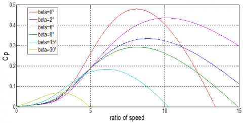
Since the wind speed is not zero after the wind turbine, only a percentage of the captured power is converted. This percentage is given by the coefficient Cp which depends on the speed ratio λ and the blade angle β.
In order to obtain the maximum power of the wind system the Cp_max should be optimized [9]. The Cp curves given in Figure 1 are obtained from Eq. (2). It can be seen that the coefficient Cp decrease when blade angle β increase. The maximum power coefficient Cp_max= 0.47 is reached when λ=8.1 and the blade angle β=0.
Figure 1. Power coefficient for wind systems
Figure 2. MPPT control for wind turbine model
The maximum power point tracking (MPPT) algorithm control for wind turbines is given by Figure 2. The concept is to determinate the speed of the turbine which allows obtaining the maximum power generated. The optimal speed turbine is given by:
$\Omega_{t_{-} o p t}=\frac{\lambda_{o p t} . v}{R}$ (6)
The mechanical speed is controlled by the electromagnetic torque Tm as shown in the following equation:
$T_{m}=\left(\Omega_{\text {mec_ref }}-\Omega_{\text {mec }}\right) . R E G$ (7)
The reference mechanical speed is obtained from the optimal turbine speed as follow:
$\Omega_{\text {mec_ref }}=G . \Omega_{t_{-} o p t}$ (8)
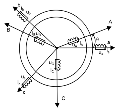
The double fed induction generator (DFIG) is represented by Figure 3. (a,b,c) and (A,B,C) denotes the stator and the rotor phases respectively, where the phase angle between the phases is 120°, θ represent the instantaneous relative position between stator and rotor magnetic axis.
Figure 3. Schematic representation of DFIG
The classical voltages equations of DFIG are given by [11]:
$\left[V_{a b c}\right]=R_{s}\left[i_{a b c}\right]+\frac{d}{d t}\left[\varphi_{a b c}\right]$ (9)
$\left[V_{A B C}\right]=R_{r}\left[i_{A B C}\right]+\frac{d}{d t}\left[\varphi_{A B C}\right]$ (10)
where,
$\left[\begin{array}{l}V_{a b c}\end{array}\right]=\left[\begin{array}{lll}V_{a} & V_{b} & V_{c}\end{array}\right]^{T}$,$\left[\varphi_{a b c}\right]=\left[\begin{array}{lll}\varphi_{a} & \varphi_{b} & \varphi_{c}\end{array}\right]^{T}$, $\left[i_{a b c}\right]=\left[\begin{array}{lll}i_{a} & i_{b} & i_{c}\end{array}\right]^{T}$ , $\left[\begin{array}{l}V_{A B C}\end{array}\right]=\left[\begin{array}{lll}V_{A} & V_{B} & V_{C}\end{array}\right]^{T}$, $\left[\varphi_{A B C}\right]=\left[\begin{array}{lll}\varphi_{A} & \varphi_{B} & \varphi_{C}\end{array}\right]^{T}$, $\left[\begin{array}{l}i_{A B C}\end{array}\right]=\left[\begin{array}{lll}i_{A} & i_{B} & i_{C}\end{array}\right]^{T}$
The total flux equations are expressed by:
$\left[\varphi_{a b c}\right]=\left[L_{s}\right]\left[i_{a b c}\right]+\left[L_{s r}\right]\left[i_{A B C}\right]$ (11)
$\left[\varphi_{A B C}\right]=\left[L_{r}\right]\left[i_{A B C}\right]+\left[L_{r s}\right]\left[i_{a b c}\right]$ (12)
where,
[Ls]: stator inductance matrix, [Lr]: rotor inductance matrix.
[Lsr]: stator-rotor mutual inductance matrix.
From Eq. (9), Eq. (10), Eq. (11), and Eq. (12) we obtain:
$\left[V_{a b c}\right]=R_{s}\left[i_{a b c}\right]+\left[L_{s}\right] \frac{d}{d t}\left[i_{a b c}\right]+\frac{d}{d t}\left\{\left[L_{s r}\right]\left[i_{A B C}\right]\right\}$ (13)
$\left[V_{A B C}\right]=R_{r}\left[i_{A B C}\right]+\left[L_{r}\right] \frac{d}{d t}\left[i_{A B C}\right]+\frac{d}{d t}\left\{\left[L_{r s}\right]\left[i_{a b c}\right]\right\}$ (14)
The equations of the DFIG in the PARK frame d-q are given by [12]:
$\left\{\begin{array}{l}\mathrm{V}_{\mathrm{ds}}=\mathrm{R}_{\mathrm{s}} \mathrm{i}_{\mathrm{ds}}+\dot{\varphi}_{\mathrm{ds}}-\omega_{\mathrm{s}} \varphi_{\mathrm{qs}} \\ \mathrm{V}_{\mathrm{qs}}=\mathrm{R}_{\mathrm{s}} \mathrm{i}_{\mathrm{qs}}+\dot{\varphi}_{\mathrm{qs}}+\omega_{\mathrm{s}} \varphi_{\mathrm{ds}} \\ \mathrm{V}_{\mathrm{dr}}=\mathrm{R}_{r} \mathrm{i}_{\mathrm{dr}}+\dot{\varphi}_{\mathrm{dr}}-\omega_{r} \varphi_{\mathrm{qr}} \\ \mathrm{V}_{\mathrm{qr}}=\mathrm{R}_{r} \mathrm{i}_{\mathrm{qr}}+\dot{\varphi}_{\mathrm{qr}}+\omega_{r} \varphi_{\mathrm{dr}}\end{array}\right.$ (15)
With: $\omega_{r}=\omega_{s}-\omega$
$\left\{\begin{array}{l}\varphi_{\mathrm{ds}}=\mathrm{L}_{\mathrm{s}} \mathrm{i}_{\mathrm{ds}}+\mathrm{Mi}_{\mathrm{dr}} \\ \varphi_{\mathrm{qs}}=\mathrm{L}_{\mathrm{s}} \mathrm{i}_{\mathrm{qs}}+\mathrm{Mi}_{\mathrm{qr}} \\ \varphi_{\mathrm{dr}}=\mathrm{L}_{\mathrm{r}} \mathrm{i}_{\mathrm{dr}}+\mathrm{Mi}_{\mathrm{ds}} \\ \varphi_{\mathrm{qr}}=\mathrm{L}_{\mathrm{r}} \mathrm{i}_{\mathrm{qr}}+\mathrm{Mi}_{\mathrm{qs}}\end{array}\right.$ (16)
where:
Rs, Rr: stator and rotor resistances respectively.
Ls, Lr: stator and rotor inductances respectively.
M: mutual inductance.
The electromagnetic torque is expressed by:
$T_{\mathrm{e}}=\mathrm{p}\left(\varphi_{\mathrm{ds}} \dot{1}_{\mathrm{qs}}-\varphi_{\mathrm{qs}} \dot{1}_{\mathrm{ds}}\right)$ (17)
From Eq. (14) it can be seen that the currents and fluxes are strongly coupled. In order to get a decoupled control of stator powers, the use of vector control is necessary. For that the stator flux is oriented along d axis.
The voltage and the frequency are supposed constant:
$\left\{\begin{array}{c}\varphi_{\mathrm{ds}}=\varphi_{\mathrm{s}} \\ \varphi_{\mathrm{qs}}=0\end{array}\right.$ (18)
From Eq. (16) and Eq. (18), we obtain the stator current as follows:
$\left\{\begin{array}{c}\mathrm{I}_{\mathrm{ds}}=\frac{\varphi_{\mathrm{ds}}-M \mathrm{I}_{\mathrm{dr}}}{L_{\mathrm{s}}} \\ \mathrm{I}_{\mathrm{qs}}=\frac{-M \mathrm{I}_{\mathrm{qr}}}{L_{\mathrm{s}}}\end{array}\right.$ (19)
Then the electromagnetic torque becomes:
$T_{\mathrm{em}}=-\frac{p M}{L_{s}} \varphi_{\mathrm{s}} \mathrm{i}_{\mathrm{qr}}$ (20)
In wind turbine systems the power of generators is medium or high, this means that the value of the stator resistance can be neglected. By considering that the flux is constant, the stator voltage will be:
$\left\{\begin{array}{c}\mathrm{V}_{\mathrm{ds}}=0 \\ \mathrm{~V}_{\mathrm{qs}}=\mathrm{V}_{\mathrm{s}}=\omega_{\mathrm{s}} \varphi_{\mathrm{ds}}\end{array}\right.$ (21)
The active and reactive powers are respectively defined as [12]:
For the stator:
$\left\{\begin{array}{l}\mathrm{P}_{\mathrm{s}}=\mathrm{V}_{\mathrm{ds}} \mathrm{i}_{\mathrm{ds}}+\mathrm{V}_{\mathrm{qs}} \mathrm{i}_{\mathrm{qs}} \\ \mathrm{Q}_{\mathrm{s}}=\mathrm{V}_{\mathrm{qs}} \mathrm{i}_{\mathrm{ds}}-\mathrm{V}_{\mathrm{ds}} \mathrm{i}_{\mathrm{qs}}\end{array}\right.$ (22)
And for the rotor:
$\left\{\begin{array}{c}\mathrm{P}_{\mathrm{r}}=\mathrm{V}_{\mathrm{dr}} \mathrm{i}_{\mathrm{dr}}+\mathrm{V}_{\mathrm{qr}} \mathrm{i}_{\mathrm{qr}} \\ \mathrm{Q}_{\mathrm{r}}=\mathrm{V}_{\mathrm{qr}} \mathrm{i}_{\mathrm{dr}}-\mathrm{V}_{\mathrm{dr}} \mathrm{i}_{\mathrm{qr}}\end{array}\right.$ (23)
By substituting Eq. (18) and Eq. (21) in Eq. (22) we obtain:
$\left\{\begin{array}{c}P_{\mathrm{s}}=-\mathrm{V}_{\mathrm{s}} \frac{M}{L_{\mathrm{s}}} \mathrm{I}_{q r} \\ Q_{\mathrm{s}}=\frac{\mathrm{V}_{\mathrm{s}} \varphi_{\mathrm{s}}}{L_{\mathrm{s}}}-\frac{\mathrm{V}_{\mathrm{s}} M}{L_{\mathrm{s}}} \mathrm{I}_{d r}\end{array}\right.$ (24)
From Eq. (24) it can be seen that the q-axis current can be used to control the active power, and the d-axis current can be used to control the reactive power. It means that the control of the active and reactive power is decoupled.
In order to be able to control the machine, the relationship between the currents and rotor voltages applied to the machine should be established.
By substituting Eq. (19) in Eq. (16) we obtain the rotor fluxes:
$\left\{\begin{array}{c}\varphi_{\mathrm{dr}}=\left(\mathrm{L}_{\mathrm{r}}-\frac{M^{2}}{L_{s}}\right) \mathrm{i}_{\mathrm{dr}}+\frac{M V_{s}}{L_{s} \omega_{s}} \\ \varphi_{\mathrm{qr}}=\left(\mathrm{L}_{\mathrm{r}}-\frac{M^{2}}{L_{s}}\right) \mathrm{i}_{\mathrm{qr}}\end{array}\right.$ (25)
The obtained flux expressions are then substituted in Eq. (15); by using the Laplace transform we obtain:
$\left\{\begin{array}{c}V_{\mathrm{dr}}=R_{r} \mathrm{i}_{\mathrm{dr}}+\left(\mathrm{L}_{\mathrm{r}}-\frac{M^{2}}{L_{s}}\right) s \mathrm{i}_{\mathrm{dr}}-g \omega_{s}\left(\mathrm{~L}_{\mathrm{r}}-\frac{M^{2}}{L_{s}}\right) \mathrm{i}_{\mathrm{qr}} \\ V_{\mathrm{qr}}=R_{r} \mathrm{i}_{\mathrm{sr}}+\left(\mathrm{L}_{\mathrm{r}}-\frac{M^{2}}{L_{s}}\right) s \mathrm{i}_{\mathrm{qr}}+g \omega_{s}\left(\mathrm{~L}_{\mathrm{r}}-\frac{M^{2}}{L_{s}}\right) \mathrm{i}_{\mathrm{dr}}+g \omega_{s}\left(\frac{M V_{s}}{\omega_{s} L_{s}}\right)\end{array}\right.$ (26)
From Eq. (26) the rotor current can be deduced and substituted in Eq. (24) we obtain the final expressions of stator powers:
$\left\{\begin{array}{c}P_{s}=-V_{s} \frac{M}{L_{s}} \frac{V_{q r}-g \omega_{s}\left(\mathrm{~L}_{\mathrm{r}}-\frac{M^{2}}{L_{s}}\right) \mathrm{i}_{\mathrm{dr}}-g \omega_{s}\left(\frac{M V_{s}}{\omega_{s} L_{s}}\right)}{R_{r}+\left(L_{r}-\frac{M^{2}}{L_{s}}\right) s} \\ Q_{s}=\frac{V_{s} \varphi_{s}}{L_{s}}-V_{s} \frac{M}{L_{s}} \frac{V_{d r}+g \omega_{s}\left(\mathrm{~L}_{\mathrm{r}}-\frac{M^{2}}{L_{s}}\right) \mathrm{i}_{\mathrm{qr}}}{R_{r}+\left(L_{r}-\frac{M^{2}}{L_{s}}\right) s}\end{array}\right.$ (27)
The Eq. (27) shows first order transfer functions for the active and reactive stator powers expressed by [13]:
$T F=\frac{M V_{s}}{L_{s} R_{r}+s L_{s}\left(L_{r}-\frac{M^{2}}{L_{s}}\right)}$ (28)
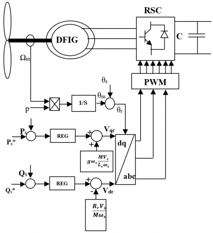
The control scheme of stator active and reactive powers is given by Figure 4.
Figure 4. DFIG control
The RST controller’s structure provides a design method, for reference tracking and disturbance rejection. Usually, the pole placement technique is used to determinate the polynomial D(p), calculate S(p) and R(p) as stated by Bezout's equation [14].
$D(p)=A(p) S(p)+B(p) R(p)$ (29)
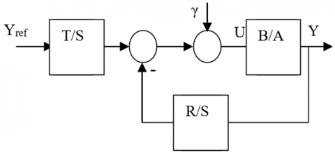
The RST controller block diagram is shown in Figure 5. where: S, R and T represent the controller polynomials.
Figure 5. RST controller structure
The relationship between the input and the output is:
$Y=\frac{B}{A}(U+\gamma)$ (30)
The control law is defined by:
$U=\frac{T}{S} Y_{r e f}-\frac{R}{S} Y$ (31)
With:
R= r0+r1.p+r2.p2+……+rn.pn
S= s0+s1.p+s2.p2+……+sn.pn
T= t0+t1.p+t2.p2+……+tn.pn
Closed loop transfer function is:
$Y=\frac{B T}{A S+B R} Y_{r e f}+\frac{B S}{A S+B R} \gamma$ (32)
To get good performance, the choice of the polynomials orders is important. A strictly proper regulator is chosen which mean if deg (A) is n than:
$\left\{\begin{array}{c}\operatorname{deg}(D)=2 n+1 \\ \operatorname{deg}(S)=\operatorname{deg}(A)+1 \\ \operatorname{deg}(R)=\operatorname{deg}(A)\end{array}\right.$ (33)
However, the polynomials forms are given by the following equations:
$\left\{\begin{array}{c}A=a_{1} p+a_{0} \\ B=b_{0} \\ D=d_{3} p^{3}+d_{2} p^{2}+d_{1} p+d_{0} \\ R=r_{1} p+r_{0} \\ S=s_{2} p^{2}+s_{1} p\end{array}\right.$ (34)
With: $A=L_{s} R_{r}+p L_{s}\left(L_{r}-\frac{M^{2}}{L_{s}}\right) ; B=M V_{s}$.
The objective is to determinate the coefficients of each polynomial; a robust placement pole strategy is used which give:
$D(s)=C F=\left(p+\frac{1}{T_{c}}\right) \cdot\left(p+\frac{1}{T_{f}}\right)^{2}$ (35)
where:
$P_{c}=-\frac{1}{T_{c}}$ is the pole of C (control pole) and $P_{f}=-\frac{1}{T_{f}}$ represents the double pole of F (filter pole).
The control pole Pc is usually chosen 2 to 5 times bigger than the pole PA. Pf is selected 3 to 5 times greater than Pc [15].
The identification between Bezout equation and Eq. (34) gives a system of four equations:
$\left[\begin{array}{l}d_{3} \\ d_{2} \\ d_{1} \\ d_{0}\end{array}\right]=\left[\begin{array}{cccc}a_{1} & 0 & 0 & 0 \\ 0 & a_{1} & 0 & 0 \\ 0 & a_{0} & b_{0} & 0 \\ 0 & 0 & 0 & b_{0}\end{array}\right]\left[\begin{array}{c}s_{2} \\ s_{1} \\ r_{1} \\ r_{0}\end{array}\right]$ (36)
For the determination of polynomial T coefficients, we consider S (0)=0 and $\lim _{p \rightarrow 0} \frac{B T}{A S+B R}=1$ (Yref = Y in steady state) then we have: T=hF.
With $h=\frac{R(0)}{F(0)}$; polynomial T is obtained as follow:
$T=t_{2} p^{2}+t_{1} p+t_{0}$ (37)
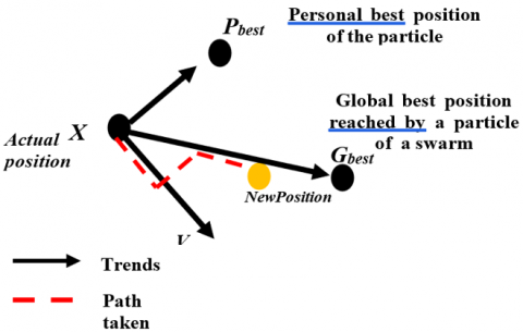
PSO is a progressive algorithm that investigates a group of candidate solutions to obtain an optimal solution for problems. This latter is measured by a fitness function. This algorithm is inspired by the collective and synchronous movement of birds’ flight. This method is considered as a progressive algorithm with a populace of agents named particles i. these latter are dispersed in the problem space [16]. Firstable, a swarm is randomly dispersed in the search area, as shown in Figure 6; the particles have also a random speed.
Figure 6. Movement principle of a particle
After that, at each time step, a particle can judge the quality of its position and remember the best position reached so far.
The particle can also ask a certain number of her congeners and obtain from them their own best performance. So each particle changes its speed and moves according to this information. In the D-dimensional search area, a particle i is represented by its position vector (X) and its speed vector (V); formulated as follows:
$X_{i}=\left(x_{i 1}, x_{i 2}, \ldots, x_{i n}\right)$ (38)
$V_{i}=\left(v_{i 1}, v_{i 2}, \ldots, v_{i n}\right)$ (39)
The assessment of her position quality is stopped by the fitness function value at this point. It is important that this particle can memorize the best position through which it has already passed, formulated as follows:
$P_{i}=\left(p_{i 1}, p_{i 2}, \ldots, p_{i n}\right)$ (40)
The equation of a particle movement for each iteration (iter) is:
$v_{i}^{\text {iter }+1}=x\left(\omega . v_{i}^{\text {iter }}+c_{1} . r_{1}^{i t e r}\left(P_{i}^{i t e r}-X_{i}^{i t e r}\right)+c_{2} . r_{2}^{i t e r}\left(P_{g}^{\text {iter }}-X_{i}^{\text {iter }}\right)\right)$ (41)
where,
$\omega$: Coefficient of inertia.
c1, c2: Acceleration coefficients which control the attraction at its best and at the best overall respectively.
r1, r2 € [0, 1]: uniform random variables.
The update of the particle position is done through the following equation:
$X_{i}^{\text {iter }+1}=X_{i}^{\text {iter }}+V_{i}^{\text {iter }+1}$ (42)
Figure 7. Estimation of the error on the solution between measured values Umes and reference values Uref
The method consists of fitting a digital model to the reference curve by iterative modifications of the input parameters until the output values reproduce the reference data (Figure 7).
The model programming and the results validation were conducted by Simulink/Matlab. This part consists on evaluating the optimal polynomial parameters of RST regulator with PSO. The PSO algorithm optimizes s1, s2, r1, r0, t2 and t1 in Eq. (36) and Eq. (37) such that overshoot D, steady state error E and rise times tr are minimized.
The preprocessing data was performed with the "Min-max" function. The behavior of the algorithm is influenced by the population size which was set at 200 particles. Where, a small amount of population doesn’t allow the good functioning of the algorithm. If c1, c2 are too small, the algorithm will explore slowly, which degrades its performance. Experience has shown that with a value of 2.05 often achieves the best results [17]. According to the study [18] the coefficient of inertia is chosen between 0.5 and 1. In our study we have chosen a value of 0.5 that we consider suitable.
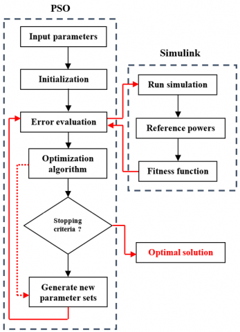
The PSO begins to look for a solution, belonging to a research space. These values are then injected into Simulink (Figure 8). The difference between the result of the measured and the reference curve is evaluated by the fitness function. The values of s1, s2, r1, r0, t2 and t1 are then modified until the fitness function (Eq. (43)) is minimized.
$f_{\min }=\int_{0}^{\infty}\left(U_{r e f}-U_{m e s}\right)^{2}(t) d t=\int_{0}^{\infty}(e)^{2}(t) d t$ (43)
The process is repeated until the difference between the measured values and the reference values is minimal or a maximum number of iterations are achieved.
Figure 8. Schematic steps of proposed RST controllers with PSO algorithm
The performances of the proposed controller are evaluated and simulated in MATLAB/Simulink environment for 1.5 MW wind turbine system. In this paper the boundary conditions are described as the wind speed profile where the minimum wind speed for the wind turbine operation is 4m/s and the rated wind speed is 12 m/s. Controllers will be tested in reference tracking and disturbances sensibility. Both mechanical and electrical parts will be considered for the study.
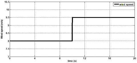
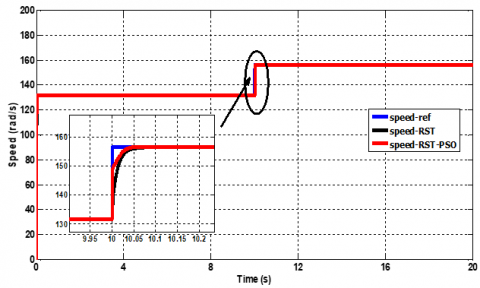
For the mechanical part two wind profiles are applied. The first one is a step change speed profile (Figure 9) and the second one is a random wind profile (Figure 11). The obtained results are shown in Figures 10 and 12 where the PSO-RST controller has a quicker response than the RST controller. The parameters of the studied system are given in the Appendix.
From Figure 12 it can be seen that the PSO-RST controller has better tracking performance where the steady-state error in speed rotation Ω is smaller than the RST controller. Both regulators show no overshoot.
Figure 9. Wind profile
Figure 10. Rotation speed
Figure 11. Random wind profile
Figure 12. Speed rotor for random wind profile
Figure 13. Rotation speed
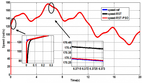
In the electrical part, the active and reactive stator powers are controlled as shown in Figure 4. To test the disturbances rejection performances we applied a step wind profile that change instantly the rotation speed from 145 rad/s to 160 rad/s as shown in Figure 13.
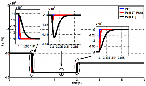
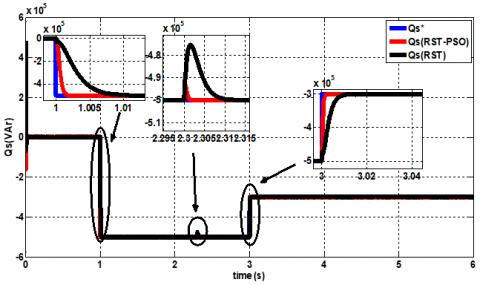
The active and reactive stator powers and their references are shown in Figures 14 and 15 respectively. From these figures it can be seen that the RST-PSO controller gives better performances where it offers a good disturbance rejection and a quicker response than the RST controller.
Figure 14. Stator active power
Figure 15. Stator reactive power
In this work we propose a method to control DFIG wind turbine conversion system where the PSO algorithm is used to determinate RST polynomial parameters. The performances of the PSO-RST controller have been evaluated and compared to the regular RST controller. The obtained results show that the proposed controller improves the performances of the system where it gives better disturbance rejection and quicker response.
|
s |
turbine rotor area, m2 |
|
v |
wind speed, m/s |
|
Cp |
power coefficient |
|
Pt |
power turbine |
|
R |
Radios of the blade, m |
|
Greek symbols |
|
|
ρ |
air density, kg/m3 |
|
$\beta$ |
blade angle, ° |
|
λ |
ratio between the blade speed and wind speed |
Table 1. Controller’s parameters (mechanical part)
|
|
RST |
RST-PSO |
|
s2 |
3.185 |
3.52 |
|
s1 |
4270.43 |
9359.85 |
|
r1 |
880261 |
406749.6 |
|
r0 |
63291139 |
21348490.86 |
|
t2 |
192 |
1955.849 |
|
t1 |
220032 |
296110.225 |
|
t0 |
63291139 |
21348490.86 |
Table 2. Controller’s parameters (electrical part)
|
|
RST |
RST-PSO |
|
s2 |
245700 |
245700 |
|
s1 |
590590121 |
730544099.108 |
|
r1 |
303704.72 |
2503710.407 |
|
r0 |
42941492.21 |
949142099.1981 |
|
t2 |
38.2 |
48.2 |
|
t1 |
81006.4 |
82017 |
|
t0 |
42941492.21 |
949142099.1981 |
Table 3. DFIG parameters
|
|
DFIG |
|
Power |
1.5 MW |
|
Rs |
0.012 Ω |
|
Rr |
0.021 Ω |
|
Ls |
0.0137 H |
|
Lr |
0.0136 H |
|
M |
0.0135 H |
|
J |
1000 kg.m2 |
|
f |
0.0024 |
|
p |
2 |
[1] Liu, X.J., Han, Y.Z. (2014). Sliding mode control for DFIG-based wind energy conversion optimization with switching gain adjustment. Proceeding of the 11th World Congress on Intelligent Control and Automation, Shenyang, China, pp. 1213-1218. https://doi.org/10.1109/WCICA.2014.7052892
[2] Martinez, M.I., Susperregui, A., Tapia, G., Camblong, H. (2011). Sliding-mode control for a DFIG-based wind turbine under unbalanced voltage. IFAC Proceedings Volumes, 44(1): 538-543. https://doi.org/10.3182/20110828-6-IT-1002.00854
[3] Aroussi, H.A., Ziani, E., Bossoufi, B. (2020). Backstepping approach applied to the DFIG-WECS. International Meeting on Advanced Technologies in Energy and Electrical Engineering, 2020: 18. https://doi.org/10.5339/qproc.2019.imat3e2018.18
[4] Amin, I.K., Uddin, M.N. (2020). Nonlinear control operation of DFIG-based WECS incorporated with machine loss reduction scheme. IEEE Transactions on Power Electronics, 35(7): 7031-7044. https://doi.org/10.1109/TPEL.2019.2955021
[5] Boualouch, A., Frigui, A., Nasser, T., Essadki, A., Boukhriss, A. (2014). Control of a doubly-fed induction generator for wind energy conversion systems by RST controller. International Journal of Emerging Technology and Advanced Engineering, 4(8): 94-98.
[6] Elmansouri, A., El mhamdi, J., Boualouch, A. (2016). Wind energy conversion system using DFIG controlled by back-stepping and RST controller. 2016 International Conference on Electrical and Information Technologies (ICEIT), Tangiers, Morocco, pp. 312-318. https://doi.org/10.1109/EITech.2016.7519612
[7] De Almeida, R.G., Lopes, J.A.P., Barreiros, J.A.L. (2004). Improving power system dynamic behavior through doubly fed induction machines controlled by static converter using fuzzy control. IEEE Trans Power Syst, 19(4): 1942-1950. https://doi.org/10.1109/TPWRS.2004.836271
[8] Altun, H., Sunter, S. (2013). Modeling, simulation and control of wind turbine driven doubly-fed induction generator with matrix converter on the rotor side. Electrical Engineering, 95: 157-170. https://doi.org/10.1007/s00202-012-0250-x
[9] Moualdia, A., Mahoudi, M., Nezli, L., Bouchhida, O. (2012). Modelling and control of a wind power conversion system based on the double-fed asynchronous generator. International Journal of Renewable Energy Research, 2(2): 300-306. https://doi.org/10.20508/ijrer.v2i2.193.g118
[10] Cárdenas, R., Pena, R., Wheeler, P., Clare, J., Munoz, A., Sureda, A. (2013). Control of a wind generation system based on a Brushless Doubly-Fed Induction Generator fed by a matrix converter. Electric Power System Reaserch, 103: 49-60. https://doi.org/10.1016/j.epsr.2013.04.006
[11] Chemidi, A., Meliani, S.M., Benhabib, M.C. (2015). Performance analysis of DFIG wind power system fed by matrix converter. Electrotehnica, Electronica, Automatica (EEA), 63(1): 78-87.
[12] Abdelghafour, H., Abderrahmen, B., Samir, Z., Riyadh, R. (2019). Hybrid type-2 fuzzy sliding mode control of a doubly-fed induction machine (DFIM). Advances in Modelling and Analysis C, 74(2-4): 37-46. https://doi.org/10.18280/ama_c.742-401
[13] Amrane, F., Chaiba, A., Francois, B., Babes, B. (2017). Experimental design of stand-alone field oriented control for WECS in variable speed DFIG-based on hysteresis current controller. 15th International Conference on Electrical Machines, Drives and Power Systems. (ELMA), Sofia, Bulgaria, pp. 304-308. https://doi.org/10.1109/ELMA.2017.7955453
[14] Rached, B., Elharoussi, M., Abdelmounim, E. (2020). Design and investigations of MPPT strategies for a wind energy conversion system based on doubly fed induction generator. International Journal of Electrical and Computer Engineering, 10(5): 4770-4781. http://doi.org/10.11591/ijece.v10i5.pp4770-4781
[15] Poitiers, F., Machmoum, M., Le Doeuff, F., Zaim, M.E. (2001). Control of a doubly-fed induction generator for wind energy conversion systems. IEEE Trans, Renewable Energy, 3(3): 373-378.
[16] Eberhart, R., Kennedy, J. (1995). A new optimizer using particle swarm theory. Proceedings of the Sixth International Symposium on micro machine and human science, Nagoya, Japan, pp. 39-43. https://doi.org/10.1109/MHS.1995.494215
[17] Bourouis, M., Zadjaoui, A., Djedid, A. (2020). Contribution of two artificial intelligence techniques in predicting the secondary compression index of fine-grained soils. Innovative Infrastructure Solutions, 5: 96. https://doi.org/10.1007/s41062-020-00348-1
[18] Eberhart, Shi, Y.H. (2001). Particle swarm optimization: developments, applications and resources. Proceedings of the 2001 Congress on Evolutionary Computation (IEEE Cat. No.01TH8546), 1: 81-86. https://doi.org/10.1109/CEC.2001.934374