Gaetani-Liseo Margot* | Alonso Corinne | Jammes Bruno
© 2021 IIETA. This article is published by IIETA and is licensed under the CC BY 4.0 license (http://creativecommons.org/licenses/by/4.0/).
OPEN ACCESS
This paper presents a study about power profiles of micro-grid with highly intermittent sources and their impacts on energy storage system (ESS). The first step of the work consists in generating the ESS power profiles thanks to a new optimal sizing algorithm. Our approach allows to size the ESS and the renewable energy sources (RES) using a power/energy considerations to generate charging and discharging profiles regardless ESS specifics parameters. In a second step, we review the potential damages on Valves Regulated Lead Acid Batteries (VRLAB). This technology has been chosen because it is the most used ESS in case of stationary applications for urban MG with RES integration. We propose some criterion to quantify the batteries stresses generated by MG working operations. Therefore, we give recommendations to enhance the VRLAB lifetime in both micro-grid design and energy management. Our method has been applied to the photovoltaic production and lighting network consumption profiles of the LAAS-CNRS building integrated photovoltaic. We compare four possible configurations of ESS and RES: two determined thanks to Pareto optimisation method and two critical cases corresponding to the minimal and the maximal values of ESS size into all the possible configuration tested.
battery ageing mechanisms, cycle lifetime, charge protocol, energy storage, Lead-acid battery, micro-grid, PV, VRLA batteries
With climate change, the fossil resources depletion and environmental considerations for planet preservation the main challenge is to found a clean and efficient way to produce and distribute the electrical energy. Research interests in micro-grid (MG) integrated to building field has gained a wide international attention during the last few years [1-3]. The considered MG are constituted of distributed power generation, as renewable energy sources (RES), associated with energy storage systems (ESS), and connected or not to the main distribution grid. To be competitive these new MG have to be efficient and sustainable while they ensure the supply of the consumption [4]. The main technical difficulties to design these MG is to deal with RES intermittencies, depending on climate conditions, while we optimize the sustainability of the ESS thanks to energy/power management systems (EMS/PMS) [5, 6]. We consider in first approach that improving the sustainability of an ESS is to enhance the lifetime to reduce the cost in an overall point of view. However, ESS lifetime depends on the energy flow during operation and so it depends both on the EMS and on the ESS sizing, which are themselves related [7, 8]. Thus, the main problematic in MG conception becomes how to define the optimal configuration between the RES and the ESS sizes (energy, power, topology and technology) taking into account the EMS and PMS associated. In addition, it seems important to consider the ESS stress mechanisms involving potentials degradations and therefore prematurely decreasing the ESS lifetime.
With this context we propose as first approach a methodology to RES and ESS sizing in case of self-sufficient application without taking into account an EMS to manage the main grid access. With a MG simulation including ESS model it would be possible to add a more complex EMS. This EMS will allow to reduce the ESS and RES sizes by purchasing power from the main grid. In the meantime, the optimal results of the sizing methodology presented in this paper, allows us to analyse the potential energy flow through the ESS independently of the ESS model. We can also use this optimal solution as the initial configuration for EMS optimization research. Thanks to these profiles we can identify the operating conditions causing benefits or stress factors on ESS and then establish the best ESS management strategy we will apply into the EMS.
We qualify the profile variations in order to compare them to the potential damages on valve regulated lead acid batteries (VRLAB). Indeed, for stationary applications in building MG, the technologies of ESS commonly used are electrochemical storage as VRLAB or Li-ions batteries [9, 10]. Although VRLAB have a limited C-rate in discharging and Li-ion technologies knowing an important increase in the last decade [11], lead acid technology maintaining its interest in the ESS market for four reasons [10, 12, 13]:
However, the main drawback of VRLAB technology is their short lifetime in case of RES operating conditions in particular with high and numerous intermittencies implying frequent incomplete cycles at partial state of charge (pSOC). To contribute on increasing the VRLAB lifetime two approaches exist. The first one consists in studying new materials or batteries geometry, and the other one consists on managing the power flow through the batteries. With this paper we contribute in this last research field.
In section 2, we give the concept and the algorithm of the methodology proposed to build the ESS profiles.
In section 3, we present the VRLAB behaviours and damages, and we give the working conditions that we have to privilege or avoid to improve the battery lifetime.
In section 4, we detail the results on our sizing methodology in case of MG dedicated to a lighting network supply, in building integrated photovoltaic (BiPV). In this section we propose different analysis according to criterion in order to qualify the damages on VRLAB.
Finally in section 5, we conclude about our work and we give some perspectives.
2.1 General sizing methodology
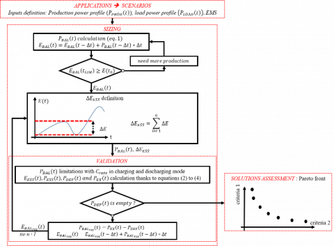
Figure 1 presents the flow char diagram for the proposed algorithm. We define PBAL(t), in equation 1, as the difference between the production power profile and the consumption power profile, respectively PPROD(t) considered positive and PLOAD(t) considered negative. PBAL(t) is negative when the loads need to be supplied.
$P_{B A L}(t)=P_{P R O D}(t)+P_{L O A D}(t)$ (1)
As shown in Figure 1, we use the EBAL(t) profile, calculated thanks to PBAL(t), to estimate the bigger decrease, ∆E, on the energy profile. Before calculating it, we verify that the EBAL(t) profile at a certain time tLIM in the time horizon T, is superior or at least equal to the energy at the beginning of the time horizon, t0. This condition ensure that production is sufficient to charge the ESS at time tLIM. The time horizon tLIM depends on the autonomy that the user wants. Next, we can estimate ∆E on the EBAL(t) profile. ∆E is the quantity of energy that the ESS has to supply to ensure the autonomy, if we consider the ESS as ideal, with an efficiency equal to unity and no limit on power rate. At the end of the first iteration, we obtain ∆EESS equal to ∆E. After this step, the verification block allows to calculate the power exchanged with the ESS, noted PESS(t). This profile depends on the limitations introduced in the algorithm, and it corresponds to the part of the power profile PBAL(t) exchanged through the ESS, having the size ∆EESS. Thanks to equations systems (2) and (3), we calculate respectively PESS(t) and EESS(t). In (2) and (3) the first parts of these equations are for charging and the second ones for discharging.
We use an energy/power consideration with constant power limitation and energy efficiency. In Eq. (2), CrateMAXc and CrateMAXd parameters are the maximum C-rate in charge and discharge. ηE is the energy efficiency of the ESS, applied at the charge, in the first equation of the system equations (3). We fix these values according to datasheet, and then with this model it is easy to test different ESS.
Figure 1. Flow chart diagram of the proposed sizing methodology algorithm
$\left\{\begin{array}{c}P_{E S S}(t)=P_{B A L}(t) \\ { if }\,\, P_{B A L}(t) \leq { Crate }_{M A X c} * \Delta E_{E S S} \\ P_{E S S}(t)=P_{B A L}(t) \\ { if }\,\, P_{B A L}(t) \geq- { Crate }_{M A X d} * \Delta E_{E S S}\end{array}\right.$ (2)
$\left\{\begin{array}{c}E_{E S S}(t)=E_{E S S}(t-\Delta t)+\eta_{E} * P_{E S S}(t-\Delta t) \\ E_{E S S}(t)=E_{E S S}(t-\Delta t)+P_{E S S}(t-\Delta t)\end{array}\right.$ (3)
Then, we can calculate the deficit and the excess power, noted respectively PDEF(t) and PEX(t), according to Eq. (4).
$P_{E S S}(t)=P_{B A L}(t)-P_{E X}(t)-\mathrm{P}_{D E F}(t)$ (4)
The configuration is validated when PDEF(t) is equal to zero in all the time steps of the horizon considered. Because of the power and energy limitations and the ESS efficiency added between the assessments of PBAL(t) and PESS(t), it is possible that we have to do two iterations to achieve the right value of ∆EESSto be autonomous. In these cases, we add to the first ∆EESS value, the estimated ∆E defined thanks to a new balance profile equal to the sum of PEX(t) and PDEF(t). This loop in the complete algorithm is presented in Figure 1, from the validation bloc to the ΔEESS definition bloc. The validated configuration corresponds to the value of ∆EESS we have to install, associated to a certain quantity of production, in order to ensure self-sufficiency.
At the end of the algorithm, the solution assessment block (Figure 1) allows to choose the optimal configuration between all the validated configurations and according to different criterion defined by the user. The final configuration selected can be defined as the optimal configuration for self-sufficient and off-grid applications or, in future works, as the initial configuration in case of connected MG, as explained in section 1.
As show in Figure 1, for each configuration we can express the energy flow into the ESS, EESS(t) by integrating PESS(t), and then the SoC in terms of energy, SoCE(t), according to Eq. (5).
$\operatorname{SoC}_{E}(t)=\frac{\mathrm{E}_{\mathrm{ESS}}(t)}{\Delta E_{E S S}}$ (5)
In our case, we propose to use the Pareto multi-objective optimization method to define the optimal configuration. Thus, as explained in Refs. [17, 18], we can define the optimal compromise between all the criterion as the point in the Pareto front which have the minimal Euclidian distance to the utopia configuration. This point represents a configuration which is impossible to achieve with the minimum of the two (or more) criterion as coordinates.
2.2 Power profiles inputs from the ADREAM BiPV database
The optimized energy building integrated photovoltaic (BiPV) ADREAM, built in 2012, at LAAS-CNRS, FRANCE, owns a 100 kWp of PV platform and more than 6500 sensors [19] and is showed in Figure 2. Its instrumentation system allows to record each minute the consumption, the production, the temperature and the air quality of the building. Nowadays a LVDC MG is deployed into the building to supply servers and USB loads [20]. One of the objectives of this platform is to supply the DC loads of the entire building, such as electrical outlets or lighting network.
Figure 2. ADREAM BiPV with example of working rooms and sensors installed
We apply our methodology in order to size the PV platform and the ESS needed for supply the lighting network of the secondary floor of the building, occupied by office.
The power profiles inputs are:
So, in our case, Eq. (1) becomes Eq. (6).
$P_{B A L}(t)=k_{P V i} * P_{P V}(t)+P_{L O A D}(t)$ (6)
The power profiles used correspond to two years (2016 and 2017) at one minute time step, ∆t. This compromise between time step and number of years studies allows us to consider both intermittency due to cloudy days and seasonal changes, while we keep a reasonable quantity of data.
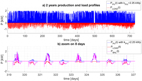
The Figure 3a shows the 2 years data set for an example of kPVi equal to 2.25 kWp.
Figure 3. Consumption data, production data and balance power profiles of the ADREAM BiPV
We can see thanks to Figure 3a the reduced PV production during the winter with an increase of the consumption in the lighting network. The Figure 3b shows a zoom on height days and the PBAL(t) profile associated to PPV(t) and PLOAD(t). We can see the production and consumption time shift on one day, with over production at the middle of the day and power deficit at the beginning and at the end of the day. We also see the PV rapid intermittency during the day, due to cloud or shadows.
In this section we explain how lead acid batteries works and what are the different damages affecting the battery and its lifetime. We give the causes of these mechanisms, and if there is any solution to avoid them. We focus on damages due to operating conditions affecting the battery efficiency and the cycle lifetime. The cycle lifetime is different to the calendar lifetime, in years, define as the battery lifetime when it is not use and impacted by temperature storage, SoC or self-discharged rate [12]. We do not consider either the potentials manufacturing damages. Finally, based on the potentials degradations listed, we determine on which power and SoC variations it is important to focus in order to qualify the VRLAB operating conditions.
3.1 Working principle of lead-acid battery
The general chemical processes occurring in lead acid batteries during charging and discharging can be explained as follows:
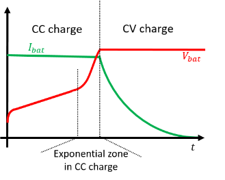
Figure 4. Typical voltage/current VRLAB characteristics during CC-CV charge
3.2 VRLAB stress factors and failure mechanisms
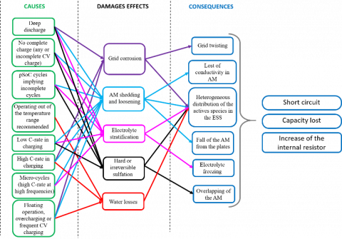
Figure 5. Potential damages with causes and consequences associated on VRLAB
According to the working principles explained previously we can bring out five main degradations processes affecting the VRLA batteries by increasing the internal resistance, involving capacity fade and potentials short circuits. The following list explains each degradations mechanisms, their causing stress factors and the uses able to minimize it. Figure 5 summarises the links between the consequences and the stress factors for each damage.
To synthesis the VRLAB damages analysis, we can see that all the consequences can affect others causes and all the damages are highly dependent and can increase other degradations. For this reason, it is very difficult to clearly do a hierarchy between damages. However, we propose to identify the main phenomenon impacting the battery cycle lifetime (prematurely reduce the battery capacity) and highlight some good practices. For example, it can be noted that operating at pSoC with incomplete cycles increases the degradation of the AM, the sulfation and the stratification. Nevertheless, this phenomenon can be reduced by regular and complete CC-CV charges. Indeed, doing a full charge with CV allows to recover some capacity and avoid hard sulfation and stratification. A patent made in 1998 by Alzieu et al. [37, 38] applies this technique to improve the battery lifetime on hybrid pack of flooded lead acid batteries, charged with RES and dedicated to ancillary services into the main distribution grid. If we consider floating state and long periods at full charge it can be noticed that the working conditions increase the corrosion effect and water losses. The deep discharge and the use at high C-rate affect the battery capacity and increase the internal resistor.
We can resume our study by giving a set of indicators helping us to identify the stress factors impacting the ESS lifetime based on the PESS(t) and the SoCE(t) profiles:
In this section we present the optimisation results following the methodology presented in section 2. We fix the time tLIM on one year over the time horizon T equal to two years. We run the algorithm in the worst case scenario by fixing the initial condition on $\Delta E_{E S S}$ equal to the first minimum of the EBAL(t) curve into the time horizon. In this way we assume that the ESS is at least one time empty during the 2 years. The variables used as criterion for the Pareto optimisation are kPVi and $\Delta E_{E S S i}$, for each i configuration. We choose to use directly these two variables, knowing that all criterion as cost or sustainability depends on these values. kPVi variable vary from 1kWp to 35kWp, with a step from 0.25 kWp, that correspond to one panel. So, we have 137 configurations, indexed by i, validated and ensuring the lightning network self-sufficient operations. We limit the C-rate in charging and discharging respectively at 0.25C and 3C, and the ESS energy efficiency, ηE, is fix at 0.85 according to the values given in [13, 39, 40].
4.1 Pareto optimization sizing results
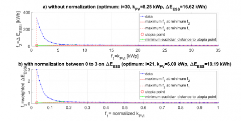
Thanks to the Pareto method we optimize both the PV size according to kPVi and the ESS size with $\Delta E_{E S S i}$. As explained in section 2, the Pareto optimisation allows to find the optimal configuration based on the minimum Euclidian distance to the utopia point. However, this optimal configuration can be different according to the normalization we made on kPVi and $\Delta E_{E S S i}$ criterion. In Figure 6, we show each configuration sizing and the Pareto optimal configuration obtained for two different types of normalization. More precisely, the Figure 6a corresponds to the Pareto curve with the real values of kPVi and $\Delta E_{E S S i}$, but the Figure 6b shows the results when kPVi and $\Delta E_{E S S i}$ are normalized, respectively between 0 to 1 and 0 to 3. Typically, it corresponds to a ratio of 3 between the kWp of PV and the kWh of ESS.
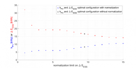
We define this ratio as a weight between kPVi and $\Delta E_{E S S i}$ and it is equal to the limit value of the $\Delta E_{E S S i}$ normalization. The choice of the weight apply on the ESS size criteria returns to the users. It can be chosen according to the ESS cost for example and the ratio between the cost of a kWp of PV and a kWh of VRLAB. In our study, if we use directly the kPVi and the $\Delta E_{E S S i}$ values, the optimal configuration obtained is the configuration with i equal to 30, and 8.25 kWp of PV plants and 16.62 kWh of batteries. The Figure 7 shows the results of the optimal configuration obtained with different normalization on $\Delta E_{E S S i}$ and kPVi . For each Pareto analysis we normalize kPVi from 0 to 1, and $\Delta E_{E S S i}$ from 0 to the $\Delta E_{E S S}$ weight. To verify the sensibility between the optimal configuration result and the weight factor, we do a variation of this weight between 1 to 15, as represented in the Figure 7 abscises axe.
The optimal configuration Pareto results converge to 10 kWp of PV panels and 14 kWh of ESS. The optimal configuration without weight and normalization (black circle) corresponds to a ratio around 9.5 between the kWp of PV installed and the kWh of ESS. This sensibility study shows the impact of the weight factors on the optimisation results. We can see that the quantity of PV increases when $\Delta E_{E S S}$ decreases and when the weight factor increases, because the results of the Pareto optimisation give a configuration with oversize PV sources in order to minimize the ESS capacity which weighs more. With this method we can adjust the optimal configuration according to the $\Delta E_{E S S}$ weight factor (normalization limit).
We choose to focus our study on the comparison of ESS power and SoCE(t) variation on four possible configurations, validated in case of self-sufficient operation, and summarized in Table 1.
Figure 6. Pareto optimization and configurations results without and with normalization on kPVi and ∆EESSi
Figure 7. Sensibility of the optimal configuration results (kPV; ∆EESS) for different normalization on ∆EESS
Table 1. Configurations saved to comparative study
|
configuration number |
i |
kPVi [kWp] |
ΔEESSi[kWh] |
configuration description |
|
1 |
1 |
1 |
332,87 |
minimum kPVi and maximum ΔEESSi ensuring autonomy |
|
2 |
30 |
8.25 |
16.62 |
optimal configuration ensuring autonomy, without normalization |
|
3 |
21 |
6 |
19.19 |
optimal configuration ensuring autonomy with normalization between 0 to 3 for ΔEESSi |
|
4 |
137 |
35 |
9.94 |
maximum kPVi and minimum ΔEESSi ensuring autonomy |
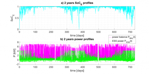
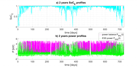
Figure 8. 2 years of power balance, ESS power and SoCE(t) profiles for the optimal configuration n° 2
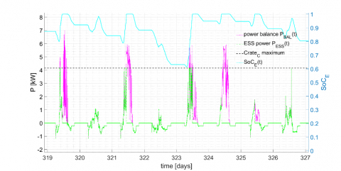
Figure 9. 8 days of power balance, ESS power and SoCE(t) profiles for the optimal configuration n° 2
Figure 10. 2 years of power balance, ESS power and SoCE(t) profiles for the optimal configuration n° 3
Figures 8 and 10 show the power exchanged with the ESS and the balance power profile (subplot b) for the two optimal configurations (2 and 3). The Figure 9 shows a zoom on 8 days of the profiles variations for the configuration 2. On these Figures the SoCE(t) profile is presented (cyan curve).
The difference between Figures 8 and 10 is the values of the ESS size normalization used for the Pareto optimisation. In Figure 8, the profiles represented correspond to the optimal configuration 2. In this case we can see that the quantity of PV is bigger than the ones in the optimal configuration 3, presented in Figure 10. This is because of the ratio between the PV kWp and the ESS kWh is around 9.5 in configuration 2 compared to 3 in configuration 3. So, regarding these two Figures, the optimal configuration 2 corresponds to a PV platform oversized. We see in Figures 8b and 9 that during charging, the PEES(t) profile is more often limitated at CrateMAXc than in configuration 3. As in consequence the PEX(t) values are important, moreover during the summer periods.
We can notice that these limitations depend on the ESS models we used and their limitations. In our case we model the power limitations by a constant power rate in charging and discharging modes, CrateMAXc and CrateMAXc. In reality, due to the voltage evolution during CC charging and discharging, and current decrease during CV charging, the power limits vary during these operating modes.
Thanks to the previous configurations cited in table 1 and the resulting ESS power and SoC profiles, we are able to identify and evaluate the stress factors implied by the working conditions on ESS, and more specifically on VRLAB.
4.2 Profiles analysis according to the VRLAB stress factors
4.2.1 C-rate impacts
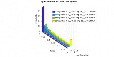
In this subsection we present our analyses of the distribution of the C-rate, during 2 years. Thanks to Figure 11, we can show that the C-rate in charging and discharging mode, respectively Cratec and Crated, depend on the configuration. In charging mode (Figure 11a) we can see that the C-rate take bigger values more often when the ΔEESS decreases. For the two optimal configurations, 2 and 3 (blue and green bars), the distribution is almost the same. For the configuration 1 (purple curve), the C-rate in charge is always smaller than 0.01C. Unlike, in the configuration 4, the C-rate in charging mode is more often between 0.24C and 0.25C, thus close to the maximum C-rate in charge.
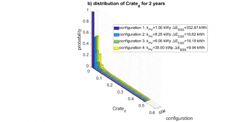
In discharging mode (Figure 11b) and for all the configurations, the C-rate is still inferior to the maximum C-rate limit, CratedMAX. Because of the strategy dedicated to improve autonomy we calculate the size of the ESS according to the more important decrease on the EESS(t) profile, so the ESS size is defined regarding an energy constraint and not a power constraint.
We can conclude that the C-rate in discharging mode is not significant if we keep the ΔEESS size as we define it thanks to the sizing methodology proposed. The C-rate in charge for the two optimal configurations (2 and 3) are distributed in all the C-rate range but mostly at low C-rate under 0.05C. It is an advantage to limit the VRLAB degradations, although it is specified that too low C-rate at the beginning of the charge can favour the AM shedding. In case of configuration 1 and 4, the C-rate distribution in charge can become an issue by using the VRLAB only with low or high C-rate.
Figure 11. Distribution of the C-rate repartition for the 4 different configurations in charging and discharging mode, for 2 years data set
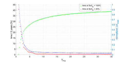
Figure 12. Cumulative time at SOCE equal to 100% or less than 30% during two years, for all the configuration
4.2.2 SoC variations
In this subsection we present the main results on the SoC fluctuations during 2 years. We are particularly interested in the time at full charge and at low SoC. We can see in Figure 12 the total time relatively to the two years data set that the ESS stay at SoCE equal to 100% (green points) or less than 30% (red points). In the right axis of the Figure 12 we report the ESS size for all the calculated and validated configurations. We see in this Figure that the duration when SoCE is lower than 30% decreases when ΔEESSi decreases and kPVi increases. Contrary the duration when SOCE is equal to 100% increases when the ΔEESSi decrease and the kPVi increase.
The first consequences seen in this Figure is that for self-sufficient operations, the damages implied by low SoC (depth discharges) are not significant because of their rarity (lower than 5% for configuration with more than 5 kWp for the kPVi value).
If we complete this observation with the SOCE(t) profile showed in Figure 8 or 10, we observe that these rates of discharge probably occur mainly during the winter.
Concerning the charge, we see that the ESS is at SOCE equal to 100% more than 25% of the time in case of configurations with kPVi is superior at 5 kWp. Full SoCE(t) mainly occur during summer. According to this observation and the mechanisms listed in section 3 it seems important to clearly define what a 100% SoCE(t) really means. With the charge model used to validate the ESS size, we do some assumption about the power limitations. Indeed, it is difficult to affirm that when the SOCE(t) profile reach to 100% the battery is fully charge and has done a complete CC-CV charge knowing that the power is limited during CV phase. Moreover, we do not know during how time the VRLAB stay at SoCE 100% between two discharges. If we assume that the full charge is reached when SoCE(t) is equal to 100%, that means that the battery operates often in floating operation mode during the two years, and it can favorise corrosion and water losses. To avoid this situation a solution could be to limit the VRLAB SoC at 80% but this limitation implies ESS oversizing and at the same time we do not use the benefit of complete recharge which regenerate the capacity loss due to sulfation and stratification, mainly cause by incomplete cycles at pSoC.
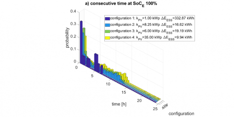
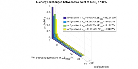
Figures 13 gives us more details about the ESS charge. Figure 13a represents the distribution of the consecutive time at SOCE(t) equal to 100%, during 2 years and for the 4 configurations. The Figure 13b shows the Watthours throughput exchanged, according to the total ESS size ΔEESS, between two time at SOCE(t) equal to 100%.
Figure 13. Distribution of the number of consecutives hours the ESS stays at SoC 100% for the 4 different configurations
For all the configurations the maximum probability corresponds to a time at full SoC less than 0.1h. So if the VRLAB is full when SoCE(t) is achieved the value of 100%, the battery does not stay a long time in floating operation and consequently the impact of corrosion and water losses can be avoided. However, it is important to control the end of the CV charge to ensure that the batteries are not overcharged during this period. In the meanwhile, if the charge process is not fully achieved when the SoCE(t) profile reach 100%, this duration do not ensure that the battery charge is complete before a new discharge.
Watthours throughput between two full charges appear to be less than 1% of the total ESS size, as show in Figure 13b. Therefore, it is difficult to conclude on the level of impact on sulfation and stratification. It would be interesting to evaluate the better compromise between the energy exchanged between two full charges and the number of full charges needed to avoid hard sulfation and stratification. This study will allow us to fix a Watthours limit ensuring the reversible sulfation phenomenon with complete CC-CV charge while we minimize the time in CV phase, when VRLAB efficiency decreases and corrosion and water losses ageing mechanisms occur.
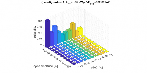
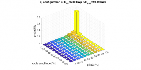
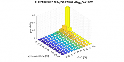
The Figure 14 shows the average pSoC during the two years calculated thanks to the SoCE(t) profile, for the 4 different configurations.
Figure 14. pSoC vs amplitude cycle histogram for each cycle of the SOCE(t) profile for 4 different configurations
We see that for the configuration 1 the cycles amplitudes on the two years are less than 10%. ESS works around the all ranges of pSoC but only doing incomplete cycles. Using the VRLAB in such conditions can cause high risk of hard sulfation and stratification.
The incomplete cycles distribution for the three other configurations (1, 2 and 3) is concentrated above pSoC equal to 50%, which is coherent with the results presented in Figure 12. This figure allows us to conclude that working at incomplete cycle around pSoC is typical of our type of application. In our case the SOC is unlimited so most of the pSoC are around 80% to 100% (more than 60% of the time between 90% to 100% of battery SoC). If we will limit the SoC at 80% the results will be a pSoC repartion mostly between 60%-80% range. In the two cases we damage the VRLAB, on one hand with corrosion and on the other hand with risking hard sulfation. Morever, by using the VRLAB between 80% to 100%, and considering that 100% represented the full charge, we mostly sollicite the battery when the effciency is low.
These figures confirm the utility of full recharge with CC-CV phases in order to recover capacity because of the stratification and sulfation mechanisms. But also confirm that we need a more accurate charge model for power limitations and to define the limit between CC and CV phases, according to the VRLAB SoC.
This paper proposes an algorithm to size the ESS and the RES for self-sufficient operation in BiPV MG. This algorithm allows to study the typical power variations without taking into account a specific ESS model. We made a comparison of the battery’s stresses implying by these power variations for four configurations ensuring the autonomy. We can see that in the cases of optimal sizing, the ESS SoC mainly stays over 60%. However, in the range 60%-100% of SoC the batteries do many incomplete cycles (with amplitude cycle less than 20% of the ESS size). The C-rate during discharging and charging and the frequency of deep-discharges do not have significant negatives impacts on ESS.
According to these observations and the potential degradations of VRLAB listed in section 3, we can conclude that stratification, AM shedding and sulfation mechanisms have to be highly considered. The risk of premature corrosion and water losses resulting of frequent operations at SoC equal to 100% must be taken into account. Moreover, as the VRLAB efficiency decrease in CV phase, as well as the potential power admitted by the battery, we preconize to limit the working operations during CV charging phase. Nevertheless, CV charging operations have positives impacts by avoiding hard sulfation and stratification, if we ensure that full charge is completely achieved.
The future challenge is to develop an accurate model of the charging to represent the power and the transition between CC and CV phases.
This will allow better knowledge of the SoC knowing the real power accepted by the battery during the CV phase.
Such a model will be very useful to manage the VRLAB charge in order to minimize the corrosion and avoid overcharges while we ensure the benefit of a complete charge.
Moreover, this model will improve our sizing algorithm by considering power limitations. We could implement in the charge model two different efficiencies during CC and CV phases. However, we have to take in mind that the power limitations model should be simple in terms of parameters identification and execution.
To manage the duration at full charge and optimize the VRLAB uses, a solution will be to split the ESS into several smaller and distributed ESS in a hybrid ESS. These smaller ESS could mainly work at pSoC around 50% to avoid corrosion and water losses, and switch between the different elements of the hybrid ESS to ensure CV phases. The sizing and the management of such hybrid ESS could be done thanks to a CC-CV charge model.
Another perspective is to search the optimal compromise between full charge benefits and corrosion phenomena. To do this it will be necessary to know the specific value of Watthours a VRLAB can delivered between two full charges. This compromise has to be analyzed with an electrochemical point of view.
|
Abbreviations |
|
|
AM |
Active Materials/Mass (in lead-acid battery) |
|
BiPV |
Building integrated PhotoVoltaic |
|
CC |
Constant Current |
|
C-rate |
Current rate |
|
CV |
Constant Voltage |
|
DC |
Direct Current |
|
EMS |
Energy Management System |
|
ESS |
Energy Storage System |
|
LVDC |
Low Voltage Direct Current |
|
MG |
Micro Grid |
|
PMS |
Power Management System |
|
pSoC |
partial State of Charge |
|
RES |
Renewable Energy Sources |
|
SoC |
State of Charge |
|
VRLAB |
Valve Regulated Lead Acid Battery |
|
Variables |
|
|
Cratec |
C-rate during ESS charging mode, C |
|
Crated |
C-rate during ESS discharging mode, C |
|
EBAL(t) |
energy balance, kWh |
|
EESS(t) |
energy flow throught the ESS, kWh |
|
kPVi |
value of PV plants installed in configuration i, kWp |
|
PBAL(t) |
power balance, kW |
|
PDEF(t) |
deficit power, kW |
|
PESS(t) |
ESS power, kW |
|
PEX(t) |
PV power in excess, kW |
|
PLOAD(t) |
load power, kW |
|
PPROD(t) |
production power, kW |
|
SoCE(t) |
ESS state of charge in terms of energy |
|
DoDE(t) |
ESS depth of discharge in terms of energy |
|
∆E |
energy decrease calculated on E(t) profile, kWh |
|
∆EESSi |
energy needed in storage for configuration i, kWh |
|
Parameters |
|
|
CrateMAXc |
ESS maximum current rate in charging mode |
|
CrateMAXd |
ESS maximum current rate in discharging mode |
|
tLIM |
limit of time to verify the condition on energy profile, h |
|
t0 |
initial time |
|
T |
time horizon |
|
Δt |
time step, h |
|
ηE |
ESS energy efficiency |
|
Indices |
|
|
t |
time |
|
i |
configurations indices |
[1] Sechilariu, M., Wang, B., Locment, F. (2013). Building-integrated microgrid: Advanced local energy management for forthcoming smart power grid communication. Energy and Buildings, 59: 236-243. https://doi.org/10.1016/j.enbuild.2012.12.039
[2] Yamashita, D.Y., Vechiu, I., Gaubert, J.P. (2020). A review of hierarchical control for building microgrids. Renewable and Sustainable Energy Reviews, 118: 109523. https://doi.org/10.1016/j.rser.2019.109523
[3] Marszal, A.J., Heiselberg, P., Bourrelle, J.S., Musall, E., Voss, K., Sartori, I., Napolitano, A. (2011). Zero Energy Building–A review of definitions and calculation methodologies. Energy and Buildings, 43(4): 971-979. https://doi.org/10.1016/j.enbuild.2010.12.022
[4] Martin-Martínez, F., Sánchez-Miralles, A., Rivier, M. (2016). A literature review of Microgrids: A functional layer based classification. Renewable and Sustainable Energy Reviews, 62: 1133-1153. https://doi.org/10.1016/j.rser.2016.05.025
[5] Carpintero-Rentería, M., Santos-Martín, D., Guerrero, J.M. (2019). Microgrids literature review through a layers structure. Energies, 12(22): 4381. https://doi.org/10.3390/en12224381
[6] Zia, M.F., Benbouzid, M., Elbouchikhi, E., Muyeen, S.M., Techato, K., Guerrero, J.M. (2020). Microgrid transactive energy: Review, architectures, distributed ledger technologies, and market analysis. IEEE Access, 8: 19410-19432. https://doi.org/10.1109/ACCESS.2020.2968402
[7] Sufyan, M., Rahim, N.A., Aman, M.M., Tan, C.K., Raihan, S.R.S. (2019). Sizing and applications of battery energy storage technologies in smart grid system: A review. Journal of Renewable and Sustainable Energy, 11(1): 014105. https://doi.org/10.1063/1.5063866
[8] Gamarra, C., Guerrero, J.M. (2015). Computational optimization techniques applied to microgrids planning: A review. Renewable and Sustainable Energy Reviews, 48: 413-424. https://doi.org/10.1016/j.rser.2015.04.025
[9] Schmid, R., Pillot, C. (2014). Introduction to energy storage with market analysis and outlook. In AIP Conference Proceedings, 1597(1): 3-13. https://doi.org/10.1063/1.4878476
[10] Zakeri, B., Syri, S. (2015). Electrical energy storage systems: A comparative life cycle cost analysis. Renewable and Sustainable Energy Reviews, 42: 569-596. https://doi.org/10.1016/j.rser.2014.10.011
[11] Schmidt, O., Melchior, S., Hawkes, A., Staffell, I. (2019). Projecting the future levelized cost of electricity storage technologies. Joule, 3(1): 81-100. https://doi.org/10.1016/j.joule.2018.12.008.
[12] Palizban, O., Kauhaniemi, K. (2016). Energy storage systems in modern grids—Matrix of technologies and applications. Journal of Energy Storage, 6: 248-259. https://doi.org/10.1016/j.est.2016.02.001
[13] Gallo, A.B., Simões-Moreira, J.R., Costa, H.K.M., Santos, M.M., Dos Santos, E.M. (2016). Energy storage in the energy transition context: A technology review. Renewable and Sustainable Energy Reviews, 65: 800-822. https://doi.org/10.1016/j.rser.2016.07.028
[14] May, G.J., Davidson, A., Monahov, B. (2018). Lead batteries for utility energy storage: A review. Journal of Energy Storage, 15: 145-157. https://doi.org/10.1016/j.est.2017.11.008
[15] Sullivan, J.L., Gaines, L. (2010). A review of battery life-cycle analysis: State of knowledge and critical needs. Argonne National Lab, 10 7. https://doi.org/10.2172/1000659
[16] BCI. (2019). Battery Council International. https://batterycouncil.org/default.aspx.
[17] Cheikh, M., Jarboui, B., Siarry, P. (2010). A method for selecting Pareto optimal solutions in multiobjective optimization. Journal of Informatics and Mathematical Sciences, 2(1): 51-62. https://doi.org/10.26713/jims.v2i1.27
[18] Terlouw, T., AlSkaif, T., Bauer, C., Van Sark, W. (2019). Multi-objective optimization of energy arbitrage in community energy storage systems using different battery technologies. Applied Energy, 239: 356-372. https://doi.org/10.1016/j.apenergy.2019.01.227
[19] LAAS-CNRS. ADREAM project. https://www.laas.fr/public/fr/le-projet-adream.
[20] Dulout, J., Alonso, C., Séguier, L., Jammes, B. (2017). Development of a photovoltaic low voltage DC microgrid for buildings with energy storage systems. In ELECTRIMACS 2017, pp. 1-6.
[21] Berndt, D. (2001). Valve-regulated lead-acid batteries. Journal of Power Sources, 100(1-2): 29-46. https://doi.org/10.1016/S0378-7753(01)00881-3
[22] Linden, D. (1995). Handbook of batteries. In Fuel and Energy Abstracts, 4(36): 265.
[23] Hardman, A.M. (1988). A comparison of flooded, gelled and absorptive-separator lead/acid cells. Journal of Power Sources, 23(1-3): 127-134. https://doi.org/10.1016/0378-7753(88)80058-2
[24] Büngeler, J., Cattaneo, E., Riegel, B., Sauer, D.U. (2018). Advantages in energy efficiency of flooded lead-acid batteries when using partial state of charge operation. Journal of Power Sources, 375: 53-58. https://doi.org/10.1016/j.jpowsour.2017.11.050
[25] Cugnet, M., Liaw, B.Y. (2011). Effect of discharge rate on charging a lead-acid battery simulated by mathematical model. Journal of Power Sources, 196(7): 3414-3419. https://doi.org/10.1016/j.jpowsour.2010.07.089
[26] Valkovska, D., Dimitrov, M., Todorov, T., Pavlov, D. (2009). Thermal behavior of VRLA battery during closed oxygen cycle operation. Journal of Power Sources, 191(1): 119-126. https://doi.org/10.1016/j.jpowsour.2008.10.014
[27] Lodi, G., McDOWALL, J., Rosellini, S. (1996). VRLA battery aging characteristics. In Proceedings of Intelec'96-International Telecommunications Energy Conference, 52-58. https://doi.org/10.1109/INTLEC.1996.572378
[28] Spiers, D.J., Rasinkoski, A.D. (1995). Predicting the service lifetime of lead/acid batteries in photovoltaic systems. Journal of Power Sources, 53(2): 245-253. https://doi.org/10.1016/0378-7753(94)01989-9
[29] Ruetschi, P. (2004). Aging mechanisms and service life of lead–acid batteries. Journal of Power Sources, 127(1-2): 33-44. https://doi.org/10.1016/j.jpowsour.2003.09.052
[30] Mattera, F., Benchetrite, D., Desmettre, D., Martin, J.L., Potteau, E. (2003). Irreversible sulphation in photovoltaic batteries. Journal of Power Sources, 116(1-2): 248-256. https://doi.org/10.1016/S0378-7753(02)00698-5
[31] Jossen, A., Garche, J., Sauer, D.U. (2004). Operation conditions of batteries in PV applications. Solar Energy, 76(6): 759-769. https://doi.org/10.1016/j.solener.2003.12.013
[32] Svoboda, V., Wenzl, H., Kaiser, R., Jossen, A., Baring-Gould, I., Manwell, J., Sauer, D.U. (2007). Operating conditions of batteries in off-grid renewable energy systems. Solar Energy, 81(11): 1409-1425. https://doi.org/10.1016/j.solener.2006.12.009
[33] Ebner, E., Gelbke, M., Zena, E., Wieger, M., Börger, A. (2018). Temperature-dependent formation of vertical concentration gradients in lead-acid-batteries under pSoC operation–Part 2: Sulfate analysis. Electrochimica Acta, 262: 144-152. https://doi.org/10.1016/j.electacta.2017.12.046
[34] Meissner, E. (1999). How to understand the reversible capacity decay of the lead dioxide electrode. Journal of Power Sources, 78(1-2): 99-114. https://doi.org/10.1016/S0140-6701(00)90784-7
[35] Ebner, E., Börger, A., Gelbke, M., Zena, E., Wieger, M. (2013). Temperature-dependent formation of vertical concentration gradients in lead-acid batteries under PSoC operation–Part 1: Acid stratification. Electrochimica Acta, 90: 219-225. https://doi.org/10.1016/j.electacta.2012.12.013
[36] Jossen, A. (2006). Fundamentals of battery dynamics. Journal of Power Sources, 154(2): 530-538. https://doi.org/10.1016/j.jpowsour.2005.10.041
[37] Alzieu, J., Camps, J.C., Smimite, H. (1998). Procede de commande d’une centrale electrique associee a une source d’energie temporellement aleatoire. 98: 08531.
[38] Alzieu, J., Smimite, H., Glaize, C. (1997). Improvement of intelligent battery controller: state-of-charge indicator and associated functions. Journal of Power Sources, 67(1-2): 157-161. https://doi.org/10.1016/S0378-7753(97)02508-1
[39] Amrouche, S.O., Rekioua, D., Rekioua, T., Bacha, S. (2016). Overview of energy storage in renewable energy systems. International Journal of Hydrogen Energy, 41(45): 20914-20927. https://doi.org/10.1016/j.ijhydene.2016.06.243
[40] Poullikkas, A. (2013). A comparative overview of large-scale battery systems for electricity storage. Renewable and Sustainable Energy Reviews, 27: 778-788. https://doi.org/10.1016/j.rser.2013.07.017