Oussama Herizi* | Said Barkat
OPEN ACCESS
In this paper, a backstepping control combined with a modified space vector modulation (MSVM) for a quasi z-source inverter (QZSI) fed by a fuel cell is proposed. The QZSI employs a unique impedance network to couple the main circuit of the inverter to a proton exchange membrane fuel cell (PEMFC). This topology provides an attractive single stage DC-AC conversion with buck-boost capability unlike the traditional voltage source inverter (VSI). The MSVM is used to insert the shoot through state within the traditional switching signals in order to boost the inverter input voltage, and to keep the same performances of the traditional SVM. A DC peak voltage controller using backstepping approach is proposed to overcome the fuel cell voltage fluctuations under load changes, and to reduce the inductor current ripples as well. Comprehensive simulations are presented to prove the effectiveness and the performances of the proposed control strategy under different operating conditions.
quasi z-source inverter, modified space vector modulation, backstepping control, fuel cell
The most DC/AC power converter used in modern energy conversion systems is the voltage source inverter (VSI). However, the VSI is a buck converter, thus the output voltage range is limited to applications requiring smaller voltages than the input DC voltage. To handle this drawback, a DC/DC boost converter is necessary to step up the input DC voltage of the VSI, which is commonly required in the applications where both buck and boost voltage are demanded. Unfortunately, this leads to high cost, low efficiency, and reduced reliability of the resulting double stage conversion system. For that reason, a z-source inverter (ZSI) was proposed in [1] as an alternative power conversion concept to overcome the limitations of the traditional VSI. In the ZSI topology, two inductors and two capacitors connected in X shape are needed to couple the inverter main circuit to the DC source. Consequently, the ZSI achieves voltage buck/boost conversion in one stage, without need to extra switching devices.
On the same context, an improved z-source topology known as quasi-z-source inverter (QZSI) is considered in literature in order to control both DC link voltage and AC output voltage. This topology presents some advantages like having a continuous input current that is suitable for fuel cell applications without need to an additional filter. Also, it allows the use of the shoot-through switching states, which eliminates the need for dead-times that are used in the traditional inverter to avoid the risk of damaging the inverter circuit [1, 2]. Furthermore, for the applications where the DC input source has a wide voltage variation range such as fuel cells and batteries, QZSI is a good option. In addition to that, the QZSI has been used in many other applications such as direct-drive wind generation system, photovoltaic power system, and hybrid electric vehicles [3, 4].
On the other hand, different modulation techniques and control strategies are required to control the ZSI/QZSI to get the desired phase, frequency and amplitude of the AC output voltage. There are four important shoot-through modulation techniques commonly proposed in the literature, which are simple boost control (SBC), maximum boost control, maximum constant boost control (MCBC), and modified space vector modulation (MSVM) [5-16]. In this paper, a MSVM is adopted to insert the shoot through (ST) state within the traditional switching signals in order to boost the fuel cell voltage. This modulation technique reduces effectively the switches commutation time, decreases the output voltage/current harmonic content, and ensures better utilization of the DC-link voltage. Consequently, the voltage stress and switching losses will be reduced significantly compared to the other traditional PWM techniques [5, 6].
Controlling the ZSI/QZSI is an important issue where several closed-loop control methods have been widely studied in the literature [5-13]. There are mainly four methods to control DC-link voltage of the ZSI/QZSI, which are: direct DC-link voltage control, indirect DC-link voltage control, and unified control [10]. Indeed, in [7] the capacitor voltage was controlled by using a PID controller and the modulation index is controlled by the SBC method. While in [8] a sliding mode control method was used to control the ST duty ratio, and a PI controller combined with a neural network for a robust control was adopted in [9]. An example of connecting a bidirectional z-source inverter (BZSI) to the grid during the battery charging/discharging operation mode using a proportional plus resonance (PR) controller was demonstrated in [11]. In all aforementioned control methods, the capacitor voltage or the DC-link voltage are controlled by regulating the shoot-through duty cycle using different controller types and the output voltage is controlled by regulating the modulation index using the différents shoot-through modulation techniques.
In this paper, a dual loop capacitor voltage controller using backstepping approach for a quasi z-source inverter (QZSI) is proposed to overcome the fuel cell voltage variations under load changes, and to reduce the inductor current ripples as well. The MSVM is adopted to control the AC output voltage with less voltage/current harmonic content, and ensures better utilization of the DC-link voltage.
The paper is organized as follows: the fuel cell and QZSI modeling is introduced in section two. The MSVM technique and backstepping controllers based on Lyapunov approach are presented in section three. Section four is devoted for simulation results showing the behavior of the proposed control strategy under different operating conditions including input voltage changes, load disturbances, and steady state operation. Finally, a conclusion is pointed out in section five.
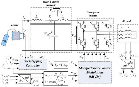
The proposed system shown in Fig.1 consists of a three-phase QZSI feeding a three-phase linear load. The DC side impedance network couples the fuel cell and the inverter to achieve voltage boost in a single stage. The peak DC-link voltage, defined as ${{\hat{V}}_{dc}}={{V}_{C1}}+{{V}_{C2}}$, is directly controlled by regulating the ST duty ratio using a backstepping approach, while the AC voltage is controlled by the modulation index using MSVM technique.
Figure 1. Backstepping control of QZSI fed by a PEMFC
2.1 Proton exchange membrane fuel cell modeling
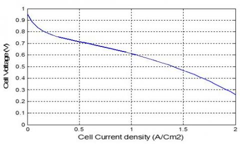
Different models of PEMFC are reported in the literature, Figure 2 shows the I(V) curve per cell. Thus, a single fuel cell can produce less than 1V. To produce a higher output voltage, multiple fuel cells are connected in series. The output fuel cell voltage ${{V}_{fc}}$ is defined as a function of the fuel cell losses [17-19], as follows
${{V}_{fc}}={{E}_{Nerst}}-{{V}_{act}}-{{V}_{ohm}}-{{V}_{conc}}$ (1)
In the above equation, ${{E}_{Nerst}}$ stands for the reversible voltage based on the Nernst equation given
${{E}_{Nerst}}=N\left[ \begin{align} & 1.229-0.85\times {{10}^{-3}}({{T}_{fc}}-298,15)+ \\ & 4,3085\times {{10}^{-5}}{{T}_{fc}}(\ln ({{P}_{H2}})+\frac{1}{2}\ln ({{P}_{O2}})) \\ \end{align} \right]$ (2)
where N is the number of cells; Tfc is the operation temperature; PH2 and PO2 are the partial pressures of hydrogen, and oxygen, respectively.
Figure 2. PEM full cell polarization curve
${{V}_{act}}$ is the activation voltage drop due to the rate of reactions on the surface of the electrodes; ${{V}_{ohm}}$ is the ohmic voltage loss from the resistances of proton flow in the electrolyte; ${{V}_{conc}}$ is the voltage loss from the reduction in concentration gases or the transport of mass of oxygen and hydrogen. Their equations are given as follows
${{V}_{act}}=N\frac{R{{T}_{fc}}}{2\alpha F}ln(\frac{{{I}_{fc}}+{{I}_{n}}}{{{I}_{o}}})$ (3)
${{V}_{ohm}}=N{{I}_{fc}}r$ (4)
${{V}_{con}}=Nm\exp (n{{I}_{fc}})$ (5)
where ${{I}_{fc}}$, ${{I}_{o}}$ and ${{I}_{n}}$ are the output current, exchange current, and internal current, respectively; $R$, $\alpha $ and F are the universal gas constant [J/gm-mol-k], charge transfer coefficient and Faraday constant [C/mole], respectively; r is the membrane and contact resistances; n and m are constants in the mass transfer voltage.
2.2 Quasi Z-source inverter modeling
The operation of the QZSI can be understood from two states: one called the shoot through (ST) state and the other called the non-shoot-through state (NST). The shoot through state appears when the inverter is shorted (two switches in the same leg are turned ON at the same time). In this sequence, the DC-link voltage (${{V}_{DC}}$) is equal to zero and the diode D is OFF, as shown in Figure 3(a). The second state is when the inverter operates in six active vectors and two zero vectors, in this case, the diode is turned ON, and the DC-link voltage is equal to (${{V}_{C1}}+{{V}_{C2}}$), as shown in Figure 3(b).
From Figure 3 and by applying Kirchhoff laws and neglecting Joule and iron losses, the state model of the QZSI fed by a fuel cell source can be obtained as
$\left\{ \begin{align} & {{L}_{1}}(d{{I}_{fc}}/dt)+M(d{{I}_{L2}}/dt)={{V}_{fc}}-{{V}_{C1}}(1-u)+{{V}_{C2}}u \\ & {{L}_{2}}(d{{I}_{L2}}/dt)+M(d{{I}_{fc}}/dt)={{V}_{C2}}(1-u)+{{V}_{C1}}u \\ & {{C}_{1}}(d{{V}_{C1}}/dt)=-{{I}_{L2}}u+{{I}_{fc}}(1-u)-{{I}_{inv}}(1-u) \\ & {{C}_{2}}(d{{V}_{C2}}/dt)=-{{I}_{fc}}u+{{I}_{L2}}(1-u)-{{I}_{inv}}(1-u) \\ \end{align} \right.$ (6)
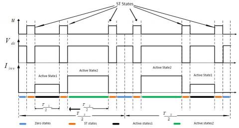
where u represents the logical control variable that takes two values according to the operating state (u=1 in shoot-through state, and u=0 in non-shoot-through state), and Iinv represents the current absorbed by the inverter during the non-shoot-through states. Note that Iinv =0 when the QZSI operates in ST state and during the application if the two zero-vector in NST states, as illustrated in Figure 4.
The averaged model of the QZSI can be written as function of the duty cycle d that represents the mean value of the control variable u, as follows
Figure 3. Operation modes of the QZSI
Figure 4. Logical command, DC-link voltage, and input current of QZSI
$\left\{ \begin{align} & {{L}_{1}}\frac{d{{I}_{fc}}}{dt}+M\frac{d{{I}_{L2}}}{dt}={{V}_{fc}}-{{V}_{C1}}(1-d)+{{V}_{C2}}d \\ & {{L}_{2}}\frac{d{{I}_{L2}}}{dt}+M\frac{d{{I}_{fc}}}{dt}={{V}_{C2}}(1-d)+{{V}_{C1}}d \\ & {{C}_{1}}\frac{d{{V}_{C1}}}{dt}=-{{I}_{L2}}d+{{I}_{fc}}(1-d)-\frac{{{V}_{\alpha }}{{I}_{\alpha }}+{{V}_{\beta }}{{I}_{\beta }}}{{{V}_{C1}}+{{V}_{C2}}} \\ & {{C}_{2}}\frac{d{{V}_{C2}}}{dt}=-{{I}_{fc}}d+{{I}_{L2}}(1-d)-\frac{{{V}_{\alpha }}{{I}_{\alpha }}+{{V}_{\beta }}{{I}_{\beta }}}{{{V}_{C1}}+{{V}_{C2}}} \\ \end{align} \right.$ (7)
where Iinv can be replaced by its mean value ${P}/{({{V}_{C1}}+{{V}_{C2}})}\;$ with $P={{v}_{a}}{{i}_{a}}+{{v}_{b}}{{i}_{b}}+{{v}_{c}}{{i}_{c}}={{V}_{\alpha }}{{I}_{\alpha }}+{{V}_{\beta }}{{I}_{\beta }}$, where (${{v}_{a}}$,${{v}_{b}}$, ${{v}_{c}}$) and (${{i}_{a}}$,${{i}_{b}}$, ${{i}_{c}}$) are the AC voltages and line currents, respectively. The QZSI has the same capacitance and inductance (C1 =C2 =C and L1 = L2 =L), so it is possible to reduce the system order by rewriting (7) as function of the capacitive voltages sum ${{V}_{C}}={{V}_{C1}}+{{V}_{C2}}$ and the inductive currents sum ${{I}_{L}}={{I}_{fc}}+{{I}_{L2}}$ [20]. Finally, the equation (7) becomes
$\left\{ \begin{align} & C\frac{d{{V}_{C}}}{dt}={{I}_{L}}(1-2d)-2\frac{{{V}_{\alpha }}{{I}_{\alpha }}+{{V}_{\beta }}{{I}_{\beta }}}{{{V}_{C}}} \\ & (L+M)\frac{d{{I}_{L}}}{dt}={{V}_{fc}}-{{V}_{C}}(1-2d) \\ \end{align} \right.$ (8)
The steady state value of the peak DC link voltage ${{\hat{V}}_{dc}}={{V}_{C}}={{V}_{C1}}+{{V}_{C2}}$ is expressed as
${{\hat{V}}_{dc}}=\frac{{{V}_{fc}}}{1-2d}=B{{V}_{fc}}$ (9)
where B is the boost factor.
$B=\frac{1}{1-2d}\ge 1$ (10)
The output peak phase voltage of the inverter can be expressed as
${{\hat{V}}_{ac}}=m\frac{{{{\hat{V}}}_{dc}}}{2}=mB\frac{{{V}_{fc}}}{2}$ (11)
Equation (11) means that the output voltage can be stepped up and down by controlling m and B.
3.1 MSVM control
The SVM for three-phase VSI is based on the representation of the voltage vectors in a two-dimensional plane. The desired output voltage can be represented by an equivalent rotating vector ${{V}_{ref}}$ [5, 6]. According to the different values of switching functions, the inverter has eight kinds of working states, including six active vectors, which are v1(001), v2(010), v3(011), v4(100), v5(101), v6(110) and two zero vectors v0(000) and v7(111), as shown in Figure 5. The αβ plane is divided in six sectors (60-degree per sector). In each sector, the switching function and time can be calculated by the two adjacent vectors to the reference one according to the following equation in which the first sector is chosen as an example.
${{V}_{ref}}={{v}_{1}}\frac{{{T}_{1}}}{{{T}_{s}}}+{{v}_{2}}\frac{{{T}_{2}}}{{{T}_{s}}}+{{v}_{0(7)}}\frac{{{T}_{0}}}{{{T}_{s}}}$ (12)
where T1 and T2 are the switching time of active states, T0 is the switching time of zero vectors (V0 or V7), given by
$\left\{ \begin{align} & {{T}_{1}}={{m}_{i}}{{T}_{s}}\sin (\frac{\pi }{3}-\theta +\frac{\pi }{3}(i-1) \\ & {{T}_{2}}={{m}_{i}}{{T}_{s}}\sin (\theta -\frac{\pi }{3}(i-1) \\ & {{T}_{0}}={{T}_{s}}-{{T}_{1}}-{{T}_{2}} \\ \end{align} \right.$ (13)
Figure 5. Traditional SVM of VSI
where i=1,2,...,6 is the sector number; Ts is the switching period; $\theta $ is the angle of the desired output voltage Vref and miis the modulation index defined as
${{m}_{i}}=\sqrt{3}\frac{{{V}_{ref}}}{{{{\hat{V}}}_{dc}}}$ (14)
The three-phase QZSI has an additional zero state when the load terminals are shorted through both the upper and lower switches of any one phase leg, any two-phase legs or all three-phase legs. This ST zero state provides the sole buck-boost attribute to the inverter. However, the insertion of ST state must not influence the ON active states, though this switching is applied during the zero state intervals; consequently the performance of the SVM is not affected. Various modified SVM control methods of QZSI are presented in the literature, a comparison between these MSVM is summarized in [6]. In this paper, the MSVM illustrated in Figure 6 is adopted in which the total shoot-through time interval is equally divided into six parts per one control cycle. In case of the first sector, for instance, the switching pulses of the MSVM are generated by the following steps
$\left\{ \begin{align} & {{T}_{\min }}={{T}_{0}}/4 \\ & {{T}_{mid}}={{T}_{0}}/4+{{T}_{1}}/2 \\ & {{T}_{\max }}={{T}_{0}}/4+{{T}_{1}}/2+{{T}_{2}}/2 \\ \end{align} \right.$ (15)
$\left\{ \begin{align}& {{T}_{\min +}}={{T}_{\min }}-{{T}_{st}}/4 \\ & {{T}_{\min -}}={{T}_{\min }}-{{T}_{st}}/12 \\ \end{align} \right.$$\left\{ \begin{align}& {{T}_{\operatorname{mi}d+}}={{T}_{\operatorname{mi}d}}-{{T}_{st}}/12 \\ & {{T}_{\min -}}={{T}_{\min }}+{{T}_{st}}/12 \\ \end{align} \right.$$\left\{ \begin{align}& {{T}_{\max +}}={{T}_{\max }}+{{T}_{st}}/12 \\ & {{T}_{\max -}}={{T}_{\max }}+{{T}_{st}}/4 \\ \end{align} \right.$ (16)
Figure 6. MSVM switching moment of three-phase QZSI
where the subscripts + and - denote the modified switching times of the upper and lower switches in one bridge leg, respectively, and Tst is the shoot-through time interval. It should be noted that the maximum shoot-through time interval has to meet (Tst ≤ T0) in order to ensure that the active state times will not be affected [5].
3.2 Backstepping control of QZSI
Backstepping method is a nonlinear control based on Lyapunov approach, where its achievement can be divided into several steps. Let us consider the state variables ${{V}_{C}}={{\hat{V}}_{dc}}$ and IL defined by
$\left\{ \begin{align} & {{{\dot{V}}}_{C}}=\frac{1}{C}[(1-2d){{I}_{L}}-2\frac{{{V}_{\alpha }}{{I}_{\alpha }}+{{V}_{\beta }}{{I}_{\beta }}}{{{V}_{C}}}] \\ & {{{\dot{I}}}_{L}}=\frac{1}{L+M}({{V}_{fc}}-{{V}_{C}}(1-2d)) \\ \end{align} \right.$ (17)
In this step, we look for the virtual control that ensures the asymptotic convergence of the capacitor voltage VC to its reference ${{\hat{V}}_{dc\_ref}}$. So the following error is introduced
${{e}_{1}}={{\hat{V}}_{dc\_ref}}-{{V}_{C}}$ (18)
By differentiating equation (18) and using (17), the following error dynamic equation can be obtained
${{\dot{e}}_{1}}={{\dot{\hat{V}}}_{dc\_ref}}-\frac{1}{C}((1-2d){{I}_{L}}-2\frac{{{V}_{\alpha }}{{I}_{\alpha }}+{{V}_{\beta }}{{I}_{\beta }}}{{{V}_{C}}})$ (19)
The amount (1-2d) can be replaced by its steady state value given by equation (9): $1-2d={{V}_{fc}}/{{\hat{V}}_{dc}}={{V}_{fc}}/{{V}_{C}}$, so the equation (19) becomes
${{\dot{e}}_{1}}={{\dot{\hat{V}}}_{dc\_ref}}-\frac{1}{C}(\frac{{{V}_{fc}}}{Vc}{{I}_{L}}-2\frac{{{V}_{\alpha }}{{I}_{\alpha }}+{{V}_{\beta }}{{I}_{\beta }}}{{{V}_{C}}})$ (20)
Let us check the tracking error stability by choosing the Lyapunov candidate function as below
${{V}_{1}}=\frac{1}{2}e_{1}^{2}$ (21)
Using the derivative of the equation (21), the virtual control reference that stabilizes the tracking error ${{e}_{1}}$ is given by
${{I}_{L\_ref}}=C\frac{{{V}_{C}}}{{{V}_{fc}}}({{K}_{1}}{{e}_{1}}+{{\dot{\hat{V}}}_{dc\_ref}})-2\frac{{{V}_{\alpha }}{{I}_{\alpha }}+{{V}_{\beta }}{{I}_{\beta }}}{{{V}_{fc}}}$ (22)
where K1 is a positive design gain introduced to influence the closed loop dynamic. The choice of the control law given by equation (22) will lead to ${{\dot{V}}_{1}}=-{{K}_{1}}e_{1}^{2}<0$, this is obviously a semi-negative definite function, so the tracking error ${{e}_{1}}$ will be stabilized.
Let us consider the following error between the inductor current and its reference value given by (22).
${{e}_{2}}={{I}_{L\_ref}}-{{I}_{L}}$ (23)
By differentiating the equation (23), the following error dynamic equation can be obtained
${{\dot{e}}_{2}}={{\dot{I}}_{L\_ref}}-\frac{1}{L+M}({{V}_{fc}}-{{V}_{C}}(1-2d))$ (24)
Now, a new Lyapunov function based on the peak DC-link voltage and inductor current errors can be defined as
${{V}_{2}}=\frac{1}{2}e_{1}^{2}+\frac{1}{2}e_{2}^{2}$ (25)
In order to make the derivative of the Lyapunov function given by (25) negative definite, the choice of ${{\dot{e}}_{2}}=-{{K}_{2}}{{e}_{2}}$ is necessary. Where K2 is a positive parameter selected to ensure that the dynamic of the inductor current is faster than the dynamic of the peak DC-link voltage. So, the duty cycle reference that stabilizes the variables Vc and IL to their desired values is given by
${{d}_{ref}}=\frac{1}{2}-\frac{{{V}_{fc}}}{Vc}+\frac{L+M}{{{V}_{C}}}({{K}_{2}}{{e}_{2}}+{{\dot{I}}_{L\_ref}})$ (26)
The choice of the control law given by (26) guarantees an asymptotic stability of the whole system since the derivative of (25) is negative definite function.
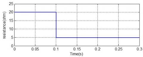
The performance of the proposed backstepping control has been tested using the parameters of the overall system listed in Table 1. To verify the robustness of the proposed control shown in Figure 1, sudden change of the load resistance at 0.1s (Figure 7) and sudden change of the modulation index reference at 0.2s (Figure 8) are introduced. Figures 9 to 11 present the simulation results of the proposed control under load disturbance and AC voltage references variation.
Table 1. System parameters
|
Item |
Parameter |
Value |
|
PEMFC |
Number of cells N |
500 |
|
Rated power Pfc_nom |
25 (kW) |
|
|
Maximum operating point [Iend,Vend] |
[75A,325V] |
|
|
Nominal supply pessure[PO2,PH2] |
[1, 1.5] (bar) |
|
|
QZSI |
QZSI inductances L1=L2 |
0.5 (mH) |
|
QZSI mutual inductance M |
0.5 (mH) |
|
|
QZSI capacitors C1=C2 |
500 (µF) |
|
|
Switching frequency f |
10 (kHz) |
|
|
DC-linkvoltage rerference Vdc_ref |
700(V) |
|
|
AC load inductance l |
2 (mH) |
|
|
AC voltage frequency f |
50 (Hz) |
|
|
|
PI Parameters [KP,KI] |
[0.6, 15] |
|
|
Backstepping Parameters[K1,K2] |
[500, 4000] |
Figure 7. AC load resistance
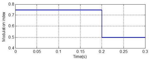
Figure 8. Modulation index reference
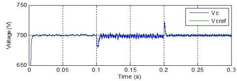
Figure 9. Peak DC-link voltage and its reference
Figure 10. PEMFC voltage Vfc
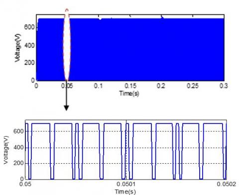
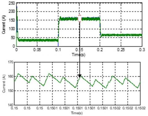
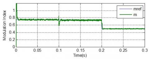
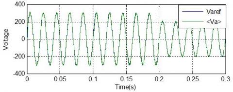
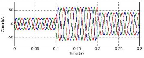
From these results, it can be noted that the peak DC-link voltage is adequately regulated to its reference with the presence of slight variations due to sudden changes in the load resistance at 0.1s and the modulation index reference at 0.2s, as shown in Figure 9. From Figure 10, it can be seen that the drop on the fuel cell voltage between 0.1 s and 0.2 s, manifested by the increasing fuel cell current presented in Figure 12, is caused by the load change. It can be seen from Figure 13 that the shoot trough duty cycle depends strongly on the fuel cell voltage variation, and it can be stated that the relationship between the peak DC-link voltage, the fuel cell voltage, and the shoot trough duty cycle is verified according to the equation 9. From Figure 15, it is clear that the shoot-through time remains less than the zero-state time independently of the introduced load and voltage variations. Furthermore the modulation index is properly regulated to its reference by the proposed MSVM-backstepping control, and the AC output voltage remains unchanged during the load increase as shown in Figures 16 and 17. From Figure 18, it is remarkable that the AC line current depends linearly on the load variation and the AC output voltage variation as well. These simulation results prove the robustness of the proposed control approach and the good dynamic of both DC and AC variables under sudden changes of the load and AC voltage reference.
Figure 11. DC-link voltage Vdc
Figure 12. Inductor current IL
Figure 13. Shoot-trough duty cycle dref
Figure 14. Modulation index and its reference
Figure 15. Shoot trough and zero times
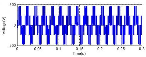
Figure 16. AC output voltage Va
Figure 17. Average AC output voltage <Va> and its reference
Figure 19 shows a comparative study between backstepping and PI controllers in which a sudden change in the three-phase resistance load is introduced between 0.2 and 0.6s. It is clearly shown that the drop voltage in the case of PI controller is more significant compared with the voltage drop with backstepping controller. On the other hand the proposed backstepping controller can achieve faster response, lower voltage ripple and better stability for the QZSI when the fuel cell and load variation is large. So, all this result demonstrates the validity of the theoretical design and the robustness of the proposed controller.
Figure 18. AC load currents
Figure 19. Disturbance rejection evaluation by using backstepping controller and PI controller
This paper has proposed a backstepping control technique combined with a modified space vector modulation for a three-phase QZSI powered by a PEMFC. In this approach, the peak DC-link voltage is controlled by regulating the ST duty ratio using a backstepping controller and the AC voltage is controlled by regulating the modulation index using a modified space vector modulation. The proposed control strategy is verified by simulation under different disturbances of the load and AC voltage reference variations. The simulation results prove the robustness of the proposed control and the good dynamic of the DC and AC variables. It is worth noticing that the proposed control method can be useful in different applications such as photovoltaic and wind power generation systems.
[1] Peng, F.Z. (2003). Z-source inverter. IEEE Transactions on Industry Applications, 39(2): 504-510. https://doi.org/10.1109/TIA.2003.808920
[2] Peng, F.Z., Shen, M., Qian, Z. (2004). Maximum boost control of the Z-source inverter. 2004 IEEE 35th Annual Power Electronics Specialists Conference (IEEE Cat. https://doi:10.1109/pesc.2004.1355751
[3] Li, Y., Jiang, S., Cintron-Rivera, J.G., Peng, F.Z. (2013). Modeling and control of quasi-z-source inverter for distributed generation applications. IEEE Transactions on Industrial Electronics, 60(4): 1532-1541. https://doi:10.1109/tie.2012.2213551
[4] Adamowicz, M., Guzinski, J., Strzelecki, R., Peng, F.Z., Abu-Rub, H. (2011). High step-up continuous input current LCCT-Z-source inverters for fuel cells. 2011 IEEE Energy Conversion Congress and Exposition. https://doi:10.1109/ecce.2011.6064070
[5] Siwakoti, Y.P., Peng, F.Z., Blaabjerg, F., Loh, P.C., Town, G.E., Yang, S. (2015). Impedance-source networks for electric power conversion Part II: Review of control and modulation techniques. IEEE Transactions on Power Electronics, 30(4): 1887–1906. https://doi:10.1109/tpel.2014.2329859
[6] Liu, Y., Ge, B., Abu-Rub, H., Peng, F.Z. (2014). Overview of space vector modulations for three-phase Z-source/quasi-Z-source inverters. IEEE Transactions on Power Electronics, 29(4): 2098–2108. https://doi:10.1109/tpel.2013.2269539
[7] Ding, X., Qian, Z., Yang, S., Cui, B., Peng, F.Z. (2007). A PID control strategy for DC-link boost voltage in Z-source inverter. APEC 07 - Twenty-Second Annual IEEE Applied Power Electronics Conference and Exposition. https://doi:10.1109/apex.2007
[8] Rajaei, A.H., Kaboli, S., Emadi, A. (2008). Sliding-mode control of z-source inverter. 2008 34th Annual Conference of IEEE Industrial Electronics. https://doi:10.1109/iecon.2008.4758081
[9] Rastegar-Fatemi, M.J., Mirzakuchaki, S., Rastegar Fatemi, S. (2008). Wide-range control of output voltage in Z-source inverter by neural network. The International Conference on Electrical Machines and Systems, ICEMS, Orlando, USA, pp.1653-1658.
[10] Ellabban, O., Van Mierlo, J., Lataire, P. (2011). Capacitor voltage control techniques of the Z-source inverter: A comparative study. EPE Journal, 21(4): 13-24. https://doi:10.1080/09398368.2011.11463806
[11] Ellabban, O., Mierlo, J.V., Lataire, P. (2011). Control of a bidirectional Z-source inverter for electric vehicle applications in different operation modes. Journal of Power Electron, 11(2): 120-131. https://doi.org/10.6113/jpe.2011.11.2.120
[12] Liang, W., Liu, Y., Ge, B., Wang, X. (2018). DC-link voltage control strategy based on multi-dimensional modulation technique for quasi-Z-source cascaded multilevel inverter photovoltaic power system. IEEE Transactions on Industrial Informatics. https://doi:10.1109/tii.2018.2863692
[13] Lv, Y., Yu, H., Liu, X. (2018). Switching control of sliding mode and passive control for DC-link voltage of isolated shoot-through Z-source inverter. 2018 Chinese Automation Congress (CAC). https://doi:10.1109/cac.2018.8623636
[14] Ellabban, O., Van Mierlo, J., Lataire, P. (2009). Comparison between different PWM control methods for different Z-source inverter topologies. The 13th European Conference on Power Electronics and Applications, Barcelona, 8-10 Sept. https://doi.org/10.6113/jpe.2011.11.2.120
[15] Rostami, H., Khaburi, D.A. (2009). Voltage gain comparison of different control methods of the Z-source inverter. International Conference on Electrical and Electronics Engineering - ELECO 2009, Bursa.
[16] Shen, M., Wang, J., Joseph, A., Peng, F.Z., Tolbert, L.M., Adams, D.J. (2006). Constant boost control of the Z-source inverter to minimize current ripple and voltage stress. IEEE Transactions on Industry Applications, 42(3), 770–778. https://doi:10.1109/tia.2006.872927
[17] Na, W. (2011). Ripple current reduction using multi-dimensional sliding mode control for fuel cell DC to DC converter applications. 2011 IEEE Vehicle Power and Propulsion Conference. https://doi:10.1109/vppc.2011.6043038
[18] Herizi, O., Barkat, S. (2016). Backstepping control and energy management of hybrid DC source based electric vehicle. 2016 4th International Symposium on Environmental Friendly Energies and Applications (EFEA). https://doi:10.1109/efea.2016.7748792
[19] Gao, D., Jin, Z., Zhang, J., Li, J., Ouyang, M. (2016). Development and performance analysis of a hybrid fuel cell/battery bus with an axle integrated electric motor drive system. International Journal of Hydrogen Energy, 41(2): 1161–1169. https://doi:10.1016/j.ijhydene.2015.10.046
[20] Battiston, A., Miliani, E.H., Pierfederici, S., Meibody-Tabar, F. (2016). Efficiency improvement of a quasi-Z-source inverter-fed permanent-magnet synchronous machine-based electric vehicle. IEEE Transactions on Transportation Electrification, 2(1): 14–23. https://doi:10.1109/tte.2016.2519349