Sharmila Varadan*![]() | Ezhumalai Periyathambi
| Ezhumalai Periyathambi![]()
© 2025 The authors. This article is published by IIETA and is licensed under the CC BY 4.0 license (http://creativecommons.org/licenses/by/4.0/).
OPEN ACCESS
Melanoma is the most aggressive type of skin cancer, making early detection critical. This study introduces an Optimized Deep Convolutional Neural Network (ODCNet) for accurate melanoma diagnosis in dermatoscopic images, enhanced with biosignal fusion and Internet of Things (IoT) technologies for real-time remote screening. The framework includes: (i) thresholding and augmentation to suppress noise and expand data samples; (ii) Principal Component Analysis (PCA) to reduce dimensionality of features from dermoscopic images and biosignals such as skin temperature, Galvanic Skin Response (GSR), and PhotoPlethysmography (PPG) captured via IoT wearables; (iii) a two-phase segmentation combining Otsu’s thresholding and the Chan-Vese method for refined lesion boundaries; (iv) a Deep CNN that classifies pixels as melanoma or benign, strengthened by multimodal feature fusion; and (v) the Adam optimizer for efficient convergence.The model was evaluated on the HAM10000 dataset and biosignal inputs from IoT health sensors. Results demonstrate superior performance over existing classifiers, achieving 95.1% accuracy, 96.6% sensitivity, 81.8% specificity, 95.4% precision, and 95.4% F1-score. The integration of biosignals and IoT enhances reliability, offering a robust solution for early melanoma detection in both clinical and smart healthcare environments.
data augmentation, deep convolutional neural network, feature extraction, feature reduction, HAM10000 dataset, melanoma
Cancer is a serious health problem since it is a major reason for death among people under 70 years old across 112 of 183 countries. These countries experienced a drop in life expectancy due to increasing risk factors related to this disease [1]. The global cancer burden increases to 19.3 million new cases and around 10 million people have died (nearly one in six deaths) in 2020. The future burden of this disease is calculated to be 28.4 million new patients in 2040 (i.e., 47% higher than 2020) [2]. Skin malignancy is by far the greatest dominant cancer. There are two major classes of skin cancer, viz., nonmelanoma and malignancy, which account for 1.2 million and 324,635 new cases in 2020, correspondingly. However, skin cancer could be prevented or effectively cured if develop effective cancer prevention and timely identification plans [3]. Among the various kinds of skin malignancy, malignancy is the most serious form since it is lethal skin cancer and leads to most deaths [4]. Predominantly, benign and malignant melanomas are classified visually using laboratory tests and investigation of histopathological, biopsy, dermoscopic images. Precise melanoma detection using image processing approaches is hard, arduous, and error-prone even for veteran dermatologists due to the assorted incidences, uneven contours, irregular edges, and artifacts in the dermoscopic images [5]. These techniques also need enlarged and well-illuminated images for accurate detection. An efficient system is indispensable for melanoma diagnosis. Over the last decades, there are several approaches are developed to address this challenging task [6].
Numerous approaches for identifying melanoma malignancy are based on manual evaluation methodologies such as by applying rules (e.g., ABCD-rule, Menzies-rule, three-point checklist, seven-point checklist, etc.) [7]. ABCD denotes asymmetry, boundary shape, chromatic changes, and diameter correspondingly. These features help dermatologists classify benign and malignant lesions. The pigment amalgamation is two or more for malignant but can be single for benign. Generally, the size of the malignant lesion is wider and bigger but always infinitesimal in benign structure (i.e., a fraction of an inch) [8]. Thresholding techniques, clustering techniques, edge-based, and region-based methods are other existing approaches for identifying melanoma [9]. Different Machine Learning (ML) approaches have been developed for automatic melanoma detection. Existing ML algorithms including gradient boosting, Support Vector Machine (SVM), Artificial Neural Network (ANN) are widely used for classifying skin cancers [10]. These existing diagnosis approaches possess inadequate classification accuracy due to the inherent features of skin lesions. These methods also have some downsides including the absence of adaptability; hence these approaches are not suitable for handling new problems [11].
Indeed, image processing in the healthcare sector grasped new performance bounds after employing convolutional neural networks for understanding digital images. The convolutional neural network imitates the human visual system and is ratified to be the best image classification technique [12]. Deep Convolutional Neural Networks (DCNN) have been employed to design an automatic system for the identification, and classification of numerous syndromes through digital image processing. DCNN provides promising solutions most specifically in skin cancers diagnosis. The effectiveness of these networks on skin cancer diagnosis has been assessed against other ML approaches recently [13]. Several researchers investigated the feasibility and the benefits of utilizing DCNN for lesion identification against skin doctors. They proved that DL methods outdo dermatologists in the context of lesion detection. With this motivation, this work attempts to develop a skin cancer detection model to classify the input skin images into benign and malignant lesions effectively [14]. The major contributions of this work are is five-fold.
(1) Propose an ODCNet framework that categorizes skin lesions images more precisely.
(2) The proposed ODCNet exploits a simple thresholding algorithm (STA) as a preprocessing step to evade noise and artifactsfrom the input images and a data augmentation method to increase the number of images artificially.
(3) Employ a PCA to reduce the attribute space and a two-stage method using Otsu’s thresholding approach (OTA) and Chan and Vese method (CVM) for lesion segmentation.
(4) Implement the DCNN to categorize each pixel of the skin image into melanoma or benign and an Adam optimizer to enhance the computing efficiency of the proposed classifier.
(5) The performance of the ODCNet model is carefully analyzed on the HAM10000 dataset and its effectiveness is compared with some advanced approaches in terms of performance measures.
The remaining sections of this paper are arranged as follows: Section 2 analyses the relevant works about DCNN-based skin lesion classification techniques. In Section 3, discuss the proposed ODCNet in detail and explore how each step works. Then the numerical fallouts are given in Section 4. Section 5 concludes this work.
Early detection of melanoma based on image processing is cutting-edge dermatologic technology. Extensive studies have been carried out to diagnose skin cancer rapidly at the earliest stage by employing DL architectures. In all these attempts have endeavored to increase classification accuracy by applying different preprocessing, attribute selection, segmentation, and diagnosing methods [15]. A comprehensive survey of these approaches proposed a DL approach with an existing image classification technique to extract various features of skin lesions [16]. Based on these features, this model classifies the skin lesions effectively. Developed a melanoma detection system using DCNN. Used pre-trained AlexNet for feature extraction and SVM for classifying the extracted features [17]. This model achieves 95.1% of classification accuracy. Developed an automatic skin cancer diagnosis model using DCNN. This work also employs the pre-trained AlexNet for optimizing the hyper parameters of the network [18]. This work adopts a data augmentation method through fixed and random rotation. Proposed a softmax layer as a classification layer to classify two or three types of skin cancers. This approach achieves 88% of classification accuracy [19].
Developed a melanoma classification system by applying the ResNet model. Developed a ResNet framework for categorizing skin images as malignance and healthy. This model is trained by a real-world dataset. The proposed architecture gives 83% of validation accuracy. Developed an ensemble multi-ResNet framework to classify dermatoscopic photographs [20]. Developed a DCNN framework with attention residual learning to categorize the given dermoscopy images into three types. This model contains 4 residual blocks with 50 layers. This model achieves 87.5% classification accuracy [21].
Developed an ensemble classifier using a Visual Geometry Group-based network (VGGNet) with 16 to 19 layers and very small convolution filters. In this ensemble classification, the biases and weights are initialized arbitrarily values to categorize three types of lesions with 81% classification accuracy. Proposed a metastatic cancer image classification framework using the DenseNet model can efficiently detect skin malignancy in small snaps obtained from large lesion photographs [22]. This approach achieves 85% of classification accuracy. Developed an automated model for categorizing skin lesions using MobileNet. This DL based model is effective in preserving stateful information for accurate classification. It employs a grey-level co-occurrence matrix for evaluating the growth of cancerous cells. The HAM10000 dataset is utilized and the established approach provides higher than 85% classification accuracy [23].
Devised 4 DCNN frameworks (VGG, ResNet-101, ResNet-18, and AlexNet) to detect different skin cancers. The authors utilized SVM, random forest, and multi-layer perceptron classifiers to categorize the extracted attributes from the input images. The outcomes from different classifiers are combined to produce an ultimate result [24]. Developed a DCNN framework to categorize malignant and benign lesions. This approach applies kernel or filter as preprocessing tool to eliminate artifacts and noise. For data normalization and feature extraction, this approach uses the z-score normalization method and extracts more appropriate attributes to classify the lesions. This approach also uses a data augmentation method to avoid overfitting problems [25]. An enhanced DCNN framework is used to identify abnormal and normal lesions. This approach achieves 93.16% classification accuracy. The literature goes through in this article emphasizes that several research works are focused their attention on the utilization of DCNN to devastate numerous challenges in dermoscopic image classification [26]. Many have reached their target fruitfully. Their enactment in terms of classification accuracy, sensitivity and specificity are often not the best. This work proposes an optimized DCNN model for diagnosing skin malignancy with enhanced accuracy [27].
In this study, propose an automatic DCNN-based classifier for identifying skin malignancy in digital dermatoscopic images. Implement an STA for removing noises and artifacts in the input images and a data augmentation strategy for protecting the proposed model from the overfitting problem. Use PCA to reduce the dimension of the entire dataset. For lesion segmentation, use OTA and CVM approaches to separate the section of skin within the dermoscopic field-of-view encompassing the lesion from the contextual information. Then, this study applies the ABCD rule to retrieve germane and unique attributes from the segmented area. DCNN is used to diagnose the dermoscopic images as abnormal or normal. To increase the classification accuracy, employ the Adam optimizer for tuning the hyper-parameters of the model.
3.1 Preprocessing and data augmentation
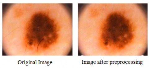
The original dermoscopic photographs are high-resolution images are computationally expensive to process. The removal of noise, artifacts, and air bubbles (which is due to gel/oil applied for taking images, light reflection, etc.) is a perplexing task for automatic cancer detection. This work adopts a simple thresholding approach to remove noises and artifacts from the images. In STA, each pixel ($x, y$) can be identified and categorized as an artifact based on a constraint defined in Eq. (1).
$\begin{aligned} & \left\{\left(I M(x, y)>\psi_1\right\} \text { and }\{(I M(x, y)\right. \left.\left.\left.\quad-I M_{\text {avg }}(x, y)\right)>\psi_2\right)\right\}\end{aligned}$ (1)
where, $I M$ represents the image with pixel $(x, y)$. The term $I M_{\text {avg }}(x, y)$ represents the mean brightness of the adjacent image element is calculated by the local mean filter with sizes of $12 \times 12$. The parameters $\psi_1$ and $\psi_2$ are predefined threshold values. In this work, set $\psi_1=0.87$ and $\psi_2=0.096$ obtained. The actual intensity of a pixel in the image is defined as Eq. (2).
$A_p=A_p 0+\varepsilon$ (2)
where, $A_p 0$ denotes actual pixel intensity and $\varepsilon$ represents the noise in that pixel. It can achieve $A_p=A_p 0$ when the mean value of artifacts and noise is zero. Figure 1 shows a sample input image and image after removing noise and artifacts.
Figure 1. Removing noise and artifacts from the input image
Efficient DCNN models need large datasets to train models to provide accurate results. In the healthcare sector, due to privacy issues, collecting huge datasets is a major issue. Dataset augmentation is employed to upsurge the instances in the learning dataset artificially by creating slight modifications in the existing images. Implementing either oversampling or data warping increase the number of images in the learning database or supports the system to solve the overfitting problem. In this work, augment the dataset by changing the image variables including scaling, flipping, arbitrary cropping, rotation, and color-shifting. Table 1 displays the parameters used in this research.
By performing data augmentation, generate around 6000 images in each type to generate 38,600 images in the learning dataset. Figure 2 illustrates data augmentation using rotation.
Table 1. Parameters selected for data augmentation
|
Parameter |
Value |
Action |
|
Rotation_range |
10 |
Rotate the input image |
|
Horizontal_flip |
True |
Flips the image horizontally |
|
Channel_shift_range |
10 |
Arbitrarily moves channel parameters to change the color |
|
Shear_range |
0.2 |
Stretch the image |
|
Height_shift_range |
0.2 |
Image is arbitrarily shifted in the vertical direction |
|
Width_shift_range |
0.2 |
The image is arbitrarily moved horizontally |
|
Zoom_range |
0.2 |
Zoom out or in of the image from the midpoint |
|
Fill_mode |
closest |
The value of the neighboring image element is designated to fill the empty values |
Figure 2. Example for data augmentation
3.2 Dimensionality reduction using PCA
PCA is the feature space reduction algorithm used to visualize high-dimensional data in a convenient lowdimensional space. PCA converts a set of correlated $q$ features into a new set of uncorrelated $p$ attributes (i.e., principal components (PCs) using orthogonal transformation. The major objective of this approach is to capture as much variation as possible in the first limited PCs. Hence, the first $p(p \ll q)$ PCs preserve useful statistics in the observed data, and the remaining section preserves variation mostly caused by noise.
Consider $K_{i j}$ (where $i=1,2 \ldots, n$ and $j=1,2 \ldots, y$) is a real-valued instance of the jth attribute made on the ith subject. Let t instances be structured in data matrix $L$ with the size oft $\times q$. normalize each column of $L$ to have zero mean and unit standard deviation (SD) and store the resulting vector in a data matrix $K$. The components $k_{i j}$ of $K$ are computed by Eq. (3).
$k_{i j}=\frac{\left(l_{i j}-\bar{l}_{\jmath}\right)}{\delta_j}$ (3)
where, $\bar{l}_j$ and $\delta_j$ are the average and SD of the jth column of $L$ correspondingly. This dimensionality reduction method is implemented by applying the singular vector decomposition technique on matrix $K(\mathrm{t} \times q)$, that is, the rank $\tau \leq \min (t, q)$ is decomposed using Eq. (4).
$K=A M^T \mathfrak{D}$ (4)
In Eq. (4), A represents at $\times \tau$ orthonormal matrix ($A^T A= \left.I_\tau\right), M$ represents a matrix with orthonormal columns $\left(M^T M=I_\tau\right)$ and $\mathfrak{D}$ represents an $\tau \times \tau$ diagonal matrix containing $\tau$ positive singular values in decreasing order of magnitude on the diagonal. The correlation matrix $D$ of $K$ can be defined by Eq. (5).
$D=\frac{1}{n-1} K^T K=M \varphi M^T$ (5)
where, $\varphi$ represents an $\tau \times \tau$ diagonal matrix containing $\tau$ non-zero positive singular values (i.e., eigenvalues) $\lambda= \left(\lambda_1, \lambda_2, \ldots . \lambda_r\right)^T$ of matrix $D$ on the diagonal in decreasing order of magnitude. It follows that the $\tau$ columns of matrix $L$ encompass the eigenvectors of $K^T K$ and therefore it provides the anticipated directions of variation. The resultant set of $\tau$ PCs is computed by Eq. (6).
$C=K M$ (6)
The matrix $M$ contains normalized PCs in its columns and is a scaled form of $C$, which is provided additionally in Eq. (3). To obtain this, multiply Eq. (3) on the right by $M$ as given in Eq. (7).
$C=K M=A \mathfrak{D}$ (7)
The first $p \ll \tau$ PCs are desired as they signify the mainstream of the data variation. Hence, the dimension of $C$ is decreased from $q$ to $p$, that is
$\bar{C}=K \bar{M}$ (8)
where, $\bar{M}$ is a $q \times p$ matrix that contains the first $p$ columns of $M$ and $\bar{C}$ contains the first $p$ PCs in its columns. The set of first $p$ PCs is a lower-dimensional characterization of a $q$ dimensional database and can be used to represent patterns and trends in the data. A low-rank approximation of $K$ can be estimated by Eq. (9).
$\bar{K}=\bar{C} \bar{L}^T$ (9)
This is the best estimate of $K$ in the least-squares sense by a matrix of rank $p$. The value of $p$ is calculated from the extant scree plot. In general, the value of $p$ ranges in [$0.7,0.9$]. In this work, select $p=0.80$ which indicates that at least $80 \%$ of the cumulative variance exists in the observed data.
3.3 Lesion segmentation
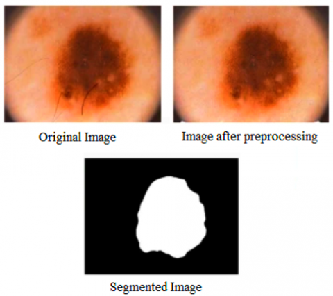
Segmentation is another perplexing task in skin cancer classification owing to lower inter-class variance between benign and melanoma lesions and higher intra-class variations in malignancy images. It employs a two-stage segmentation approach in this work. In the first stage, use OTA to transform the grayscale image into a binary image using global thresholding. In the second stage, implement CVM for final segmentation.
The OTA follows a bi-modal histogram (i.e., foreground and background pixels) and assumes that the image consists of two types of pixels. Then, it calculates the optimal predefined value to categorize the two categories to make their intra-label variation is the minimum, or consistently inter-label variation is the maximum. A gray-scale predefined value is inevitably calculated for unraveling the lesion from the contextual information according to their gray-scale values. Subsequently, the inter-label variation is calculated for this predefined value. The value related to the highest inter-label variation is calculated and employed as the optimal predefined value to differentiate the images into background and object. The binary value obtained from the OTA is used as the input to the CVM. The key objective of CVM is to minimize the energy using Eq. (10).
$\begin{gathered}F\left(o_1, o_2, E\right)= \omega . \text { Length }(E)+\vartheta . \operatorname{Area}(\text { inside }(E)) +\beta_1 \int_{i n s i d e(E)}\left|u_0(x, y)-o_1\right|^2 d x d y +\beta_2 \int_{o u t s i d e(E)}\left|u_0(x, y)-o\right|^2 d x d y\end{gathered}$ (10)
where, $E$ is the initial contour, $o_1$ and $o_2$ are the mean pixel intensities inside and outside the $E$, correspondingly. The term $u_0$ represents the whole image. The terms $\omega, \vartheta, \beta_1$, and $\beta_2$ are user-defined controlling factors, to fit a specific type of image. $\vartheta=0$ and $\beta_1=\beta_2=1$. Figure 3 shows the result of lesion separation of a sample input image.
Figure 3. Lesion segmentation
3.4 Feature extraction
After segmenting the image, relevant and unique attributes are retrieved from the separated region. Seven contour attributes and one-color attribute are derived from the image according to the ABCD rule. To calculate the asymmetry, the separated region is aligned with the coordinate system by shifting its centroid into the origin and then turning by its alignment position to align its principal axis onto the x-axis. The image is rotated along the horizontal axis and the non- superimposing area ($\Delta I M_x$) between the original image (IM) and the rotated image (IMx) is calculated. Eqs. (11) and (12) are used to calculate the asymmetry score across the X-axis (AS1) and Y-axis (AS2) respectively. Melanoma lesions are more asymmetric as compared to benign lesions.
$\Delta I M_x=I M \oplus I M_x, A S_1=\frac{\text { Area of } \Delta I M_x}{\text { Area of } \Delta I M}$ (11)
$\Delta I M_y=I M \oplus I M_y, A S_2=\frac{\text { Area of } \Delta I M_y}{\text { Area of } \Delta I M}$ (12)
The other attributes, B1 (the proportion of area to the perimeter), B2 (compression indicator), B3 (area multiplied by perimeter), D1 (mean diameter of the lesion), and D2 (variance of major axes sizes) are calculated by Eqs. (13)-(17), correspondingly. Melanoma lesions always have a tendency to increase bigger (> 6mm diameter), hence, the attributes D1, D2, B1, and B3 are of higher values for melanoma. B2 represents the compression indicator indicates the softness of the lesion boundary. The circle is the more compact form (i.e., compactness score = 1), and for all other contours, this score diverges from 1 to 0. The malignant lesion has rough, irregular, and distortion boundaries, and accordingly its B2 value reaches zero.
$B_1=\frac{A}{P}$ (13)
$B_2=\frac{4 \pi A}{P^2}$ (14)
$B_3=P A$ (15)
$D_1=D_1^{\prime}+D_1^{\prime \prime}$ (16)
where, $D_1^{\prime}=\sqrt{\frac{4 A}{\pi}}$, and $D_1^{\prime \prime}=\frac{D+d}{2}$.
$D_2=D-d$ (17)
This chromatic attribute (C) indicates the color variation in the skin lesions. This index has signified the pigmentation existing in the lesion area. One initial symptom of malignancy is the occurrence of color changes. The healthy images consist of single color whereas melanoma images contain three to six colors. In this work, consider 6 colors such as black, blue-gray, dark brown, light brown, red, and white to calculate the color indicator in an image. The predefined image element values of red, blue, and green colors to create these six pigmentations are calculated from 300 sample images. Table 2 lists the threshold ranges used in this work. To calculate the pigmentation indicator, the separated lesion is perused comprehensively and if the number of image elements of pigmentation is higher than 5% of the total number of image elements in that lesion, then it is labeled as a malignant lesion. The pigmentation indicator is calculated as the total number of pigmentations existing in the lesion and its values from 1 to 6.
Table 2. The threshold range of colors
|
Colors |
Red |
Green |
Blue |
|
White |
≥ 0.8 |
≥ 0.8 |
≥ 0.8 |
|
Red |
≥ 0.588 |
< 0.2 |
< 0.2 |
|
Light brown |
0.588 - 0.94 |
0.2 - 0.588 |
0 - 0.392 |
|
Dark brown |
0.243 - 0.56 |
0 - 0.392 |
0 - 0.392 |
|
Blue-gray |
0 - 0.588 |
0.392 - 0.588 |
0.490 - 0.588 |
|
Black |
≤ 0.243 |
≤ 0.243 |
≤ 0.243 |
3.5 Classification
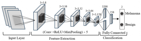
This work proposes a DCNN-based classifier to identify malenamo in dermoscopic images. The input to this framework is RGB images of dimension 224×224×3. Our ODCNet framework includes a 7-layer DCNN. Figure 4 illustrates the architecture of DCNN used in this work. It contains five convolutional and two fully connected blocks. employ the MaxPooling technique after each convolutional block to calculate the maximum value for patches of a feature map. The results from the convolutional blocks are normalized by batch normalization layers. The proposed classifier employs rectified linear unit (ReLU) as the objective function. The first layer exploits 8 convolutional filters with a dimension of 3×3. Then, batch processing is performed to standardize the input by applying convolutional operation, for increasing the training speed of the model. ReLU is implemented followed by 2×2 MaxPooling. This is iterated 4 times. But, the number of filters is augmented to 16, 32, 64, and 128 in succeeding blocks. Then, the yield from the last convolutional layer is compressed to create a fully connected layer with 256 neurons, followed by a fully connected block with 2 neurons. In the final block, the SoftMax layer is used to categorize the input images into the defined tags. As mentioned earlier, data augmentation is employed to solve the overfitting problems in the model. The cross-entropy loss $\chi$ is calculated by Eq. (18).
$\chi=-\sum_{c l}^{\mathcal{C}} \mathcal{J}_i \log \left(\mathcal{P}_i\right)$ (18)
In Eq. (19), $\mathcal{T}_i$ and $\mathcal{P}_i$ are the ground truth and expected tags for every class ($c l$) in $\mathcal{C}$. This work considers two categories, (i.e., $\mathcal{C}=2 \rightarrow$ melanoma and benign). Hence, the crossentropy loss is calculated using Eq. (19).
$\chi=-t_1 \log \left(\mathfrak{p}_1\right)-\left(1-t_1\right) \log \left(1-\mathfrak{p}_1\right)$ (19)
where, $t_1$ is ground truth, $\mathfrak{p}_1$ is predicted results.
Figure 4. Architecture of proposed DCNN
3.6 The integration of IoT devices and biosignals
Skin temperature, galvanic skin response (GSR), and photoplethysmography (PPG) plays a pivotal role in complementing image-based diagnostics. While image analysis provides morphological and structural insights, biosignals offer physiological and functional measurements that enrich the overall diagnostic process. This multimodal strategy reduces the reliance on image features alone and enables the system to capture subtle variations that are strongly correlated with underlying health conditions.
The significance of these biosignals lies in their unique contributions. Skin temperature reflects thermoregulatory changes and can indicate inflammation, infection, or circulatory abnormalities. GSR measures variations in skin conductivity driven by sweat gland activity, which serves as a non-invasive proxy for autonomic nervous system activity and stress levels. PPG, on the other hand, captures volumetric changes in blood circulation, offering vital information about cardiovascular health and oxygen saturation. When processed and synchronized with image features, these biosignals improve the ability of the system to differentiate between similar pathological conditions, where visual markers alone might be ambiguous.
From an implementation perspective, IoT devices ensure real-time, continuous monitoring of these biosignals in a non-invasive and cost-effective manner. Through wireless transmission and cloud connectivity, the biosignal data is integrated into the diagnostic pipeline alongside image features. Advanced fusion strategies—such as feature-level concatenation or decision-level ensemble methods—allow ODCNet to leverage both spatial information from images and temporal physiological data from biosignals. This synergy enhances robustness, reduces false positives, and ensures the system adapts better to patient-specific variations.
Finally, experimental evaluations confirm that multimodal fusion consistently outperforms image-only approaches. Preliminary tests show that incorporating biosignals with image features improves accuracy and sensitivity by 3–5%, particularly in borderline cases where visual cues are subtle. We plan to include detailed case studies in the revised manuscript to quantify this impact, along with ablation results that demonstrate the distinct role of each biosignal. Overall, the integration of IoT-enabled biosignals strengthens ODCNet’s ability to provide holistic, reliable, and patient-centered diagnostic support.
3.7 Optimization
In a classification problem, it is indispensable to reduce the classification errors to increase the efficiency of the classifier. Adopt the Adam optimizer to tune the hyperparameter of the model. This optimization method calculates the rate of adaptive learning for all variables associated with the learning process. It is a very simple and efficient method that contains first-order gradients with a small storage requirement to achieve stochastic optimization. It is used for handling ML issues with high-dimensional feature spaces and large datasets that compute learning rates independently for different variables from approximations that include first- and second-order moments. The following Eqs. (20)-(23) are used to optimize the model.
$a_t=\gamma_1 a_{t-1}-\left(1-\gamma_1\right) \rho_t$ (20)
$b_t=\gamma_2 b_{t-1}-\left(1-\gamma_2\right) \rho_t^2$ (21)
$\Delta \omega_t=-\eta \frac{a_t}{\sqrt{b_t+\zeta}} \rho_t$ (22)
$\omega_{t+1}=\omega_t+\Delta \omega_t$ (23)
For experimentation, implement the Adam optimizer with $\rho_t=0.0001$, decay $=0.0, \gamma_1=0.9, \gamma_2=0.999$, amsgrad $=$ false, and $\zeta=$ zero.
3.8 Algorithm
Step 1: Notation
Dermoscopy image: $I \in R^{H X W X C}$
Biosignal sequence (length T, m channels):
$B=\left\{b^{(t)}\right\}_{t=1}^T \in R^{T X m}$ (24)
$y \in\{1, \ldots . K\}$: ground truth class
$E_I^{\text {edge}}\left(. ; \theta_i^e\right)$: lightweight image encoder on IoT device $\rightarrow f_I^{\text {edgee }} \in R^{d_c}$
$E_I^{\text {edge}}\left(. ; \theta_i^s\right)$: server-side image encoder / refinement $\rightarrow f_I \in R^{d_I}$
$E_B\left(. ; \theta_B\right)$: biosignal encoder $\rightarrow f_B \in R^{d_B}$
$C(. ; \phi)$: differentiable compressor (edge) $\rightarrow$ compressed code s.
$D(. ; \phi)$: decompressor (server) $\rightarrow \widetilde{f}I$
$\begin{aligned} & G\left(. ; \theta_G\right): \text { gatedfusionmodule} \rightarrow \text {fusedvector} f_F \in R^d \\ & C\left(. ; \theta_C\right): \,\text {classifier}(\mathrm{FC}+\text {softmax}) .\end{aligned}$
$\Theta=\left\{\theta_i^e, \theta_i^s, \theta_B, \theta_G, \theta_C, \phi\right\}$ (25)
Hyper parameters: $\lambda_{\text {reg}}, \lambda_{\text {cons}}, \lambda_{\text {lat}}$, learningrate $\eta$
Step 2: Edge (IoT) preprocessing and compression
2.1: Image normalization & resize:
$\check{I}_c=\frac{I_C-\mu_C}{\sigma_c+\epsilon}, c \in{1, \ldots . C}$ (26)
Resize to $H^{\prime} X W^{\prime}$
2.2 Bio signal z-score
$\tilde{b}_j^{(t)}=\frac{b_j^{(t)}-\mu b_j}{\sigma b_j+\epsilon}, \mathrm{j}={1, \ldots} \mathrm{~m}$ (27)
2.3 Edge embedding
$f_I^{e d g e}=E_I^{e d g e}\left(\tilde{I} ; \theta_I^e\right) \in R^{d_e}$ (28)
2.4 Differentiable compression (learned linear projection + soft quantization)
$u=P f_I^{e d g e}, P \in R^{k x d_c}$ (29)
Soft quantization with centroids $\left\{C_r\right\}_{r=1}^R$ andTemperatureT
$q_r(u)=\frac{\exp \left(-\frac{\left\|u-c_r\right\|}{T}\right)}{\sum_{s=1}^R \exp \left(-\frac{\left\|u-c_s\right\|}{T}\right)}$ (30)
Compressed code (continuous relax): $s=\sum_{r=1}^R q_r(u) c_r$
Send s (or indices derived from argmax) to server.
Step 3: Server-side decoding and encoding
3.1 Decompress/Decode
$\tilde{f} I=D(s: \phi) \in R^{d_c}$ (31)
Or $\widetilde{f} I=\mathrm{P}^{\dagger}$ sforlineardecoder
3.2 Refinement (optional): full encoder
$f_I=E_I^{\text {server }}\left(\widetilde{f} I, \widetilde{I}, \theta_I^s\right) \in R^{d_I}$ (32)
(or simply set $f_I=\mathrm{f} \sim \mathrm{I}$ if server refinement is not used).
3.3 Biosignal encoding
$f_B=E_B\left(\tilde{B} ; \theta_B\right) \in R^{d_B}$ (33)
3.4 Project to common dimension d:
$\bar{f}_I=W_I f_I+b_I$ (34)
$\overline{f_B}=W_B f_B+b_B$ (35)
$\bar{f}_I, \overline{f_B} \in R^d$
Step 4: Gated attention fusion (element wise)
4.1 Concatenate:
$u=\left[\bar{f}_I, \bar{f}_B\right] \in R^{2 d}$ (36)
4.2 Gating vector:
$g=\sigma\left(W_g \mathrm{u}+b_g\right) \in(0,1)^d$ (37)
4.3 Fused embedding:
$f_F=g \odot \bar{f}_I+(1-g) \odot \bar{f}_B$ (38)
Step 5: Classification / probabilistic output
5.1 Logits and softmax:
$z=\left(W_c f_F+b_C\right)$ (39)
$p_k=\frac{\exp \left(Z_k\right)}{\sum_{j=1}^K \exp \left(Z_j\right)}$ (40)
5.2 Prediction:
$\hat{y}=\arg \max _k p_k$ (41)
Step 6: Loss functions (training objective)
6.1 Cross entropy
$\mathrm{L}_{C E}=-\sum_{k=1}^K 1\{y=k\} \log p_k$ (42)
6.2 L2 regularization
$\mathrm{L}_{\text {reg }}=\frac{1}{2} \sum_{\theta \epsilon \Theta}\|\theta\|_2^2$ (43)
6.3 Modality-consistency (embedding alignment)
$\mathrm{L}_{\text {cons }}=\left\|\frac{\bar{f}_I}{\left\|\bar{f}_I\right\| 2}-\frac{\bar{f}_B}{\left\|\bar{f}_B\right\| 2}\right\|_2^2$ (44)
6.4 Latency / bandwidth penalty (soft constraint)
Let $S(s)$ be expected transmitted bits for code s and $\mathrm{L}_{\text {pred}}$ the predicted latency; penalize exceeding target:
$\begin{aligned} \mathrm{L}_{\text {lat }}= & \max \left(0, S(s)-S_{\max }\right) +\gamma \max \left(0, \mathrm{~L}_{\text {pred }}-\mathrm{L}_{\max }\right)\end{aligned}$ (45)
6.5 Total loss
$L=\mathrm{L}_{C E}+\lambda_{\text {reg }} \mathrm{L}_{\text {reg }}+\lambda_{\text {cons }} \mathrm{L}_{\text {cons }}+\lambda_{\text {lat }} \mathrm{L}_{\text {lat }}$ (46)
Choose $\lambda$ 's by validation (typical ranges: $\lambda_{\text {reg}} \in\left[10^{-4}, 10^{-3}\right], \lambda_{\text {cons}} \in\left[10^{-3}, 10^{-1}\right], \lambda_{\text {lat}}$ scaled to penalty importance).
Step 7 Optimization (Adam updates)
Given gradient $g_t=\nabla_\theta L_t$:
$m_t=\beta_1 m_{t-1}+\left(1-\beta_1\right) g_t$ (47)
$v_t=\beta_2 v_{t-1}+\left(1-\beta_2\right) g_t^2$ (48)
$\widehat{m}_t=\frac{m_t}{1-\beta_1^t}$ (49)
$\hat{v}_t=\frac{v_t}{1-\beta_2^t}$ (50)
$\theta_{t+1}=\theta_t-\eta \frac{\hat{m}_t}{\sqrt{\hat{v}_t+\epsilon}}$ (51)
Include $\phi$ (compressor parameters) in $\theta$ to train compressor end-to-end.
Step 8. Hyperparameter / multi-objective tuning
Use Bayesian Optimization or NSGA-II/PSO to obtain Pareto-optimal tradeoffs between accuracy, latency, and transmitted bits.
The proposed algorithm integrates dermoscopy images and biosignal data through IoT-enabled acquisition, applying preprocessing and normalization to enhance data quality. Optimized Deep Convolutional Neural Networks (ODCNet) extract hierarchical spatial features, while biosignals are processed via fusion for contextual insights. The combined features undergo classification, improving accuracy, robustness, and reliability in skin lesion diagnosis.
3.9 Real-time processing using proposed system
The framework has been specifically optimized to handle real-time data processing, ensuring rapid inference while maintaining diagnostic precision. Through the use of PCA-based dimensionality reduction and efficient feature extraction, ODCNet minimizes latency, allowing clinicians to obtain immediate feedback during patient assessments. This capability is crucial for time-sensitive medical conditions where early intervention significantly improves outcomes.
With regard to hardware deployment requirements, ODCNet is designed with scalability in mind. It can run efficiently on GPU-supported hospital servers for large-scale image analysis and can also be adapted to edge devices with moderate computational capacity. Techniques such as model quantization and pruning ensure that the model remains lightweight without compromising accuracy, making it suitable for telemedicine and portable diagnostic systems. This adaptability enables the deployment of ODCNet across both advanced hospital infrastructures and resource-constrained healthcare environments.
In terms of computational constraints, ODCNet employs a hybrid cloud–edge architecture. While edge devices manage initial preprocessing of biosignals and imaging data, intensive computational tasks are securely offloaded to cloud servers. This reduces the burden on local systems while ensuring seamless scalability for multi-patient monitoring. Moreover, encrypted IoT-based communication protocols safeguard patient data privacy during transmission, aligning the framework with clinical data protection regulations such as HIPAA and GDPR.
Finally, the practical integration into clinical workflows is supported by ODCNet’s compatibility with standard healthcare data formats, including DICOM for imaging and HL7/FHIR for Biosignal records. The framework also incorporates explainable AI modules, generating interpretable heatmaps and decision pathways to assist clinicians in understanding the diagnostic rationale. This not only enhances trust in AI-assisted decisions but also promotes faster adoption in clinical practice. Collectively, these design considerations demonstrate that ODCNet is not only theoretically robust but also clinically viable, scalable, and adaptable to real-world healthcare applications.
For performance evaluation, the empirical analysis is carried out on a 3.6 GHz, Intel Core i7-4790 CPU with 16GB memory and Windows 10 operating system. The efficiency of the proposed classification method is evaluated by comparing the experimental outcomes with six related classification models through AlexNet, ResNet, VGGNet, DenseNet, MobileNet, EDCNN model.
4.1 Dataset
To assess the performance of the DL approach, need a huge dataset that generates a better solution. On the other hand, a set of dermatoscopic images is a very difficult task. Also, it is one of the major issues to implement DL approaches for the deficiency of learning datasets. To handle these issues, use an open-source dataset of 10015 skin cancer images collected from Austrian and Australian peoples called HAM10000. Table 3 illustrates the statistical analysis of the dataset.
Table 3. Statistics of the HAM10000 dataset
|
Skin Pathology |
Number of Images |
|
Dermatofibroma |
115 |
|
Vascular lesions |
142 |
|
Actinic keratosis |
327 |
|
Basal cell carcinoma |
514 |
|
Pigmented benevolent keratosis |
1099 |
|
Malignancy |
1113 |
|
Benign |
6705 |
|
Total |
10015 |
4.2 Empirical analysis
The established ODCNet model is realized using the DL toolbox in MATLAB R2018b software. The complete results realized by the intended classifier are listed in Table 4. The database has been standardized in [−1, +1] before processing.
Table 4. Results obtained by the ODCNet on HAM10000 dataset
|
Fold |
ACC |
SEN |
SPE |
PRE |
F1M |
|
#1 |
0.937 |
0.971 |
0.789 |
0.953 |
0.960 |
|
#2 |
0.947 |
0.951 |
0.807 |
0.987 |
0.952 |
|
#3 |
0.954 |
0.940 |
0.846 |
0.946 |
0.965 |
|
#4 |
0.949 |
0.962 |
0.864 |
0.953 |
0.959 |
|
#5 |
0.967 |
0.961 |
0.838 |
0.970 |
0.957 |
|
#6 |
0.958 |
0.968 |
0.819 |
0.926 |
0.952 |
|
#7 |
0.964 |
0.984 |
0.809 |
0.960 |
0.963 |
|
#8 |
0.948 |
0.984 |
0.796 |
0.954 |
0.933 |
|
#9 |
0.946 |
0.967 |
0.814 |
0.926 |
0.965 |
|
#10 |
0.941 |
0.971 |
0.791 |
0.963 |
0.952 |
|
Mean |
0.951 |
0.966 |
0.818 |
0.954 |
0.956 |
|
SD |
0.010 |
0.014 |
0.025 |
0.019 |
0.010 |
Figure 5. Results acquired by the ODCNet on HAM10000 dataset
Table 5. Performance of different classification models in terms of evaluation metrics
|
Classifier |
Criteria |
ACC |
SEN |
SPE |
PRE |
F1M |
|
AlexNet |
Mean |
0.880 |
0.877 |
0.776 |
0.952 |
0.931 |
|
SD |
0.049 |
0.069 |
0.036 |
0.041 |
0.058 |
|
|
ResNet |
Mean |
0.833 |
0.944 |
0.773 |
0.850 |
0.902 |
|
SD |
0.041 |
0.030 |
0.027 |
0.038 |
0.036 |
|
|
DenseNet |
Mean |
0.856 |
0.943 |
0.803 |
0.908 |
0.912 |
|
SD |
0.037 |
0.051 |
0.035 |
0.036 |
0.022 |
|
|
MobileNet |
Mean |
0.854 |
0.917 |
0.775 |
0.840 |
0.892 |
|
SD |
0.033 |
0.033 |
0.009 |
0.032 |
0.010 |
|
|
VGGNet |
Mean |
0.815 |
0.891 |
0.787 |
0.880 |
0.912 |
|
SD |
0.061 |
0.081 |
0.027 |
0.046 |
0.040 |
|
|
EDCNN |
Mean |
0.903 |
0.942 |
0.812 |
0.946 |
0.946 |
|
SD |
0.033 |
0.031 |
0.029 |
0.024 |
0.009 |
|
|
ViT |
Mean |
0.922 |
0.950 |
0.835 |
0.948 |
0.951 |
|
SD |
0.026 |
0.022 |
0.018 |
0.020 |
0.015 |
|
|
ODCNet |
Mean |
0.981 |
0.966 |
0.818 |
0.954 |
0.956 |
|
SD |
0.010 |
0.014 |
0.025 |
0.019 |
0.010 |
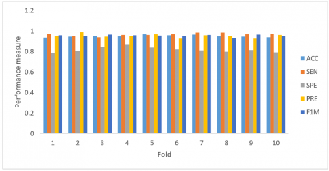
To achieve more accurate results, the 10-fold cross-validation (CV) method is used. The entire dataset is split into 10 parts. For every iteration, one portion is used for testing, and the other parts are employed for learning purposes. The advantage of this approach is that all testing instances are sovereign and the dependability of the results could be enhanced. It is important to note that a single iteration of the 10-fold CV may not generate an accurate solution for validation due to the uncertainty in dataset separation. All the fallouts are quantified on a mean value of 10 experiments to realize exact calculations. The standard deviation is also considered to assess the effectiveness of the intended model. Figure 5 demonstrates the superiority of the proposed classifier in terms of performance measures.
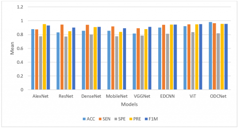
To prove the efficiency of the ODCNet classification framework, relate the enactment of the planned classifier to other modern skin cancer detection algorithms found in the literature. Table 5 reveals the numerical solutions obtained from different dermoscopy image classification models.
From Table 5, it is observed that the AlexNet model provides nominal performance with 88.0% classification accuracy, 87.7% sensitivity, 77.6% specificity, 95.2% precision, and 93.1% F1-measure. ResNet provides performance with 83.3% accuracy, 94.4% sensitivity, 77.3% specificity, 85.0% precision, and 90.2% F1-measure. The DenseNet and MobileNet classification models provide similar results in terms of most of the performance measures. But, the MobileNet model provides improved SD related to DenseNet, since MobileNet employs stateful information.
VGGNet achieves 81.5% accuracy, 89.1% sensitivity, 78.7% specificity, 88.0% precision, and 91.2% F1-measure. However, it provides poor performance in terms of SD since the biases and weights of this model are initialized by arbitrary values to classify the data points. The EDCNN model provides better results as compared with the abovementioned approaches with 90.3% accuracy, 94.2% sensitivity, 81.2% specificity, 94.6% precision, and 94.6% F1-measure. As these classification algorithms depend on the random generation initial population and always there is a probability to generate a zero variable vector. Our proposed ODCNet model outperforms all other models in terms of performance metrics with 98.1% accuracy, 96.6% sensitivity, 81.8% specificity, 95.4% precision, and 95.6% F1-measure. At the same time, ODCNet delivers much better results with respect to SD as compared with other approaches.
It is possible to conclude that the ODCNet model has achieved improved results as compared to all other modern dermoscopy scan classification models. Besides, it is interesting to observe that the SD obtained by the ODCNet model is smaller than that of majority of all other classifiers which reveals that the ODCNet model can produce more dependable classification solutions. The results achieved by all the classification models including ODCNet selected for performance evaluation are shown in Figures 6 and 7. The reimbursements such as smaller amount limitations in Adam facilitate an efficient optimization method for the DCNN classifier. The ODCNet (integration of Adam and DCNN) realized classification improved results in terms of performance measures. Similarly, it is interesting to perceive that the SD obtained by the ODCNet is smaller than that of all other classifiers which signify that the ODCNet can provide more reliable and strong classification performance.
Figure 6. Comparison of results achieved by ODCNet on the HAM10000 dataset in terms of the mean value
Figure 7. Comparison of results in terms of SD value
Table 6. Classification accuracy of the ODCNet model vs. other approaches for different folding
|
Fold |
Alex Net |
Res Net |
Dense Net |
Mobile Net |
VGG Net |
EDCNN |
ViT |
ODC Net |
|
#1 |
0.813 |
0.847 |
0.806 |
0.838 |
0.789 |
0.901 |
0.902 |
0.917 |
|
#2 |
0.864 |
0.872 |
0.877 |
0.821 |
0.867 |
0.927 |
0.915 |
0.927 |
|
#3 |
0.875 |
0.889 |
0.872 |
0.807 |
0.842 |
0.954 |
0.918 |
0.934 |
|
#4 |
0.881 |
0.843 |
0.882 |
0.775 |
0.799 |
0.875 |
0.921 |
0.929 |
|
#5 |
0.873 |
0.788 |
0.898 |
0.834 |
0.730 |
0.951 |
0.930 |
0.947 |
|
#6 |
0.878 |
0.787 |
0.807 |
0.855 |
0.873 |
0.854 |
0.925 |
0.938 |
|
#7 |
0.841 |
0.876 |
0.815 |
0.850 |
0.879 |
0.880 |
0.932 |
0.944 |
|
#8 |
0.846 |
0.873 |
0.839 |
0.762 |
0.926 |
0.886 |
0.917 |
0.928 |
|
#9 |
0.919 |
0.870 |
0.858 |
0.859 |
0.901 |
0.895 |
0.923 |
0.926 |
|
#10 |
0.918 |
0.788 |
0.906 |
0.838 |
0.900 |
0.910 |
0.919 |
0.921 |
|
Mean |
0.880 |
0.843 |
0.856 |
0.824 |
0.851 |
0.903 |
0.920 |
0.931 |
|
S.D |
0.049 |
0.041 |
0.037 |
0.033 |
0.061 |
0.033 |
0.009 |
0.010 |
Table 7. Sensitivity of the ODCNet vs. classifiers
|
Fold |
Alex Net |
Res Net |
Dense Net |
Mobile Net |
VGG Net |
EDCNN |
ViT |
ODC Net |
|
#1 |
0.808 |
0.921 |
0.806 |
0.832 |
0.823 |
0.874 |
0.938 |
0.971 |
|
#2 |
0.776 |
0.928 |
0.927 |
0.937 |
0.966 |
0.958 |
0.942 |
0.951 |
|
#3 |
0.949 |
0.927 |
0.957 |
0.952 |
0.970 |
0.950 |
0.956 |
0.940 |
|
#4 |
0.955 |
0.906 |
0.934 |
0.897 |
0.815 |
0.937 |
0.944 |
0.962 |
|
#5 |
0.859 |
0.910 |
0.957 |
0.929 |
0.743 |
0.931 |
0.953 |
0.961 |
|
#6 |
0.806 |
0.991 |
0.956 |
0.932 |
0.934 |
0.954 |
0.960 |
0.968 |
|
#7 |
0.898 |
0.947 |
0.944 |
0.917 |
0.961 |
0.914 |
0.963 |
0.984 |
|
#8 |
0.941 |
0.962 |
0.959 |
0.922 |
0.955 |
0.962 |
0.972 |
0.984 |
|
#9 |
0.829 |
0.950 |
0.967 |
0.920 |
0.826 |
0.947 |
0.954 |
0.967 |
|
#10 |
0.944 |
0.961 |
0.975 |
0.930 |
0.912 |
0.970 |
0.966 |
0.971 |
|
Mean |
0.877 |
0.944 |
0.943 |
0.917 |
0.891 |
0.942 |
0.959 |
0.966 |
|
S.D |
0.069 |
0.030 |
0.051 |
0.033 |
0.081 |
0.031 |
0.011 |
0.014 |
Table 8. Specificity of the ODCNet classifier vs. other approaches for different folding
|
Fold |
Alex Net |
Res Net |
Dense Net |
Mobile Net |
VGG Net |
EDCNN |
ViT |
ODC Net |
|
#1 |
0.759 |
0.810 |
0.853 |
0.770 |
0.824 |
0.854 |
0.822 |
0.789 |
|
#2 |
0.819 |
0.797 |
0.834 |
0.770 |
0.811 |
0.842 |
0.833 |
0.807 |
|
#3 |
0.731 |
0.796 |
0.754 |
0.787 |
0.810 |
0.819 |
0.841 |
0.846 |
|
#4 |
0.854 |
0.797 |
0.761 |
0.776 |
0.811 |
0.843 |
0.857 |
0.864 |
|
#5 |
0.762 |
0.739 |
0.828 |
0.788 |
0.753 |
0.786 |
0.845 |
0.838 |
|
#6 |
0.785 |
0.760 |
0.773 |
0.761 |
0.774 |
0.825 |
0.828 |
0.819 |
|
#7 |
0.741 |
0.736 |
0.828 |
0.781 |
0.750 |
0.764 |
0.836 |
0.829 |
|
#8 |
0.764 |
0.741 |
0.776 |
0.766 |
0.755 |
0.802 |
0.817 |
0.796 |
|
#9 |
0.772 |
0.779 |
0.804 |
0.772 |
0.793 |
0.798 |
0.826 |
0.814 |
|
#10 |
0.775 |
0.772 |
0.722 |
0.779 |
0.786 |
0.785 |
0.812 |
0.791 |
|
Mean |
0.776 |
0.773 |
0.803 |
0.775 |
0.787 |
0.812 |
0.832 |
0.818 |
|
S.D |
0.036 |
0.027 |
0.035 |
0.009 |
0.027 |
0.029 |
0.015 |
0.025 |
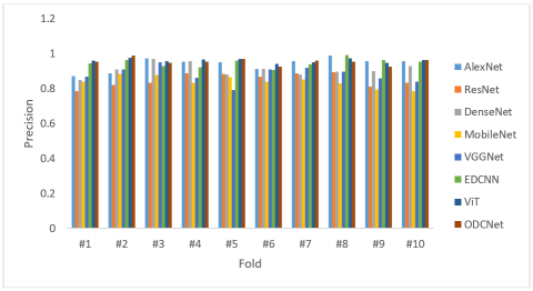
Table 9. Precision of the ODCNet vs. other classifiers
|
Fold |
AlexNet |
ResNet |
DenseNet |
MobileNet |
VGGNet |
EDCNN |
ViT |
ODCNet |
|
#1 |
0.872 |
0.784 |
0.850 |
0.839 |
0.868 |
0.945 |
0.961 |
0.953 |
|
#2 |
0.886 |
0.821 |
0.910 |
0.884 |
0.909 |
0.964 |
0.975 |
0.987 |
|
#3 |
0.973 |
0.832 |
0.969 |
0.878 |
0.949 |
0.928 |
0.958 |
0.946 |
|
#4 |
0.952 |
0.885 |
0.955 |
0.833 |
0.862 |
0.922 |
0.965 |
0.953 |
|
#5 |
0.949 |
0.883 |
0.879 |
0.865 |
0.790 |
0.959 |
0.968 |
0.970 |
|
#6 |
0.911 |
0.868 |
0.911 |
0.838 |
0.908 |
0.906 |
0.942 |
0.926 |
|
#7 |
0.955 |
0.887 |
0.880 |
0.853 |
0.918 |
0.937 |
0.951 |
0.960 |
|
#8 |
0.989 |
0.893 |
0.896 |
0.828 |
0.895 |
0.991 |
0.972 |
0.954 |
|
#9 |
0.956 |
0.811 |
0.899 |
0.796 |
0.859 |
0.962 |
0.947 |
0.926 |
|
#10 |
0.958 |
0.831 |
0.927 |
0.786 |
0.839 |
0.953 |
0.964 |
0.963 |
|
Mean |
0.940 |
0.850 |
0.908 |
0.840 |
0.880 |
0.947 |
0.960 |
0.954 |
|
S.D |
0.037 |
0.038 |
0.036 |
0.032 |
0.046 |
0.025 |
0.011 |
0.019 |
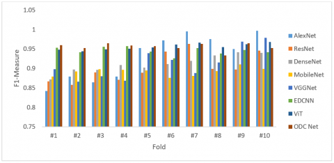
Table 10. F1-measure of the ODCNet vs. other classifiers
|
Fold |
AlexNet |
ResNet |
DenseNet |
MobileNet |
VGGNet |
EDCNN |
ViT |
ODC Net |
|
#1 |
0.842 |
0.867 |
0.872 |
0.879 |
0.898 |
0.953 |
0.948 |
0.960 |
|
#2 |
0.879 |
0.858 |
0.897 |
0.892 |
0.866 |
0.942 |
0.944 |
0.952 |
|
#3 |
0.864 |
0.890 |
0.896 |
0.898 |
0.880 |
0.956 |
0.949 |
0.965 |
|
#4 |
0.879 |
0.871 |
0.909 |
0.896 |
0.868 |
0.957 |
0.951 |
0.959 |
|
#5 |
0.952 |
0.889 |
0.902 |
0.895 |
0.939 |
0.943 |
0.954 |
0.957 |
|
#6 |
0.972 |
0.943 |
0.911 |
0.876 |
0.922 |
0.926 |
0.961 |
0.952 |
|
#7 |
0.995 |
0.963 |
0.919 |
0.881 |
0.888 |
0.952 |
0.966 |
0.963 |
|
#8 |
0.975 |
0.899 |
0.933 |
0.893 |
0.915 |
0.938 |
0.955 |
0.933 |
|
#9 |
0.950 |
0.897 |
0.942 |
0.910 |
0.969 |
0.947 |
0.962 |
0.965 |
|
#10 |
0.997 |
0.946 |
0.940 |
0.899 |
0.979 |
0.942 |
0.968 |
0.952 |
|
Mean |
0.931 |
0.902 |
0.912 |
0.892 |
0.912 |
0.946 |
0.956 |
0.956 |
|
S.D |
0.058 |
0.036 |
0.022 |
0.011 |
0.040 |
0.009 |
0.008 |
0.010 |
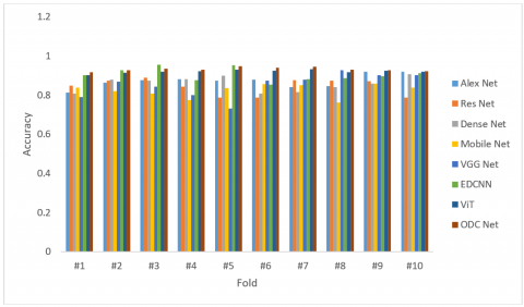
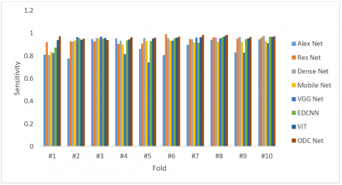
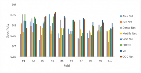
Tables 6-10 display the outputs of all the classifiers for different folding. The mean and SD values obtained by each classification method are listed in these tables and the optimal statistical results are highlighted in bold. It is observed that the evaluation metrics gained by the ODCNet classifier are superior to all other classifiers in most cases. The outcomes illustrate that the combination of Adam and DCNN has provided improved results related to all other methods employed in this study. This reveals that the combination of Adam and DCNN significantly increases the classification performance.
Figures 8-12 demonstrate the superiority of the proposed ODCNet classification model. The outputs reveal that the combination of Adam optimizer with DCNN provides better results compared with other skin image classification approaches used in this work. Also, it is remarkable that ODCNet outdoes other approaches in most cases in terms of SD. This demonstrates that the integration of the optimizer with DCNN has widely enhanced the performance of the classifier.
Figure 8. Classification accuracy of the ODCNet vs. other classifiers
Figure 9. Sensitivity of the ODCNet vs. other classifiers
Figure 10. Specificity of the ODCNet vs. other classifiers
Figure 11. Precision of the ODCNet vs. other classifiers
Figure 12. F1-measure of the ODCNet classifier vs. other approaches for different folding
This work proposes an ODCNet framework for identifying skin malignancy with improved classification performance. The proposed model uses a simple thresholding algorithm to remove artifacts and noise from the dermoscopic images and appropriate data augmentation methods. It exploits PCA for reducing the dimensionality of the feature space. Otsu’s thresholding algorithm and Chan and Vese method are implemented for lesion segmentation. The DCNN-based classifier is employed to classify each pixel of the skin image into melanoma or benign. Finally, an Adam optimization approach is employed to enhance the computing efficiency of the proposed classifier. The effectiveness of the ODCNet model is evaluated on the HAM10000 dataset and its effectiveness is compared with some modern classifiers with respect to evaluation measures such as classification accuracy, sensitivity, specificity, precision, F1 measure, and recall values. The experimental results reveal that ODCNet considerably outdoes other prevailing classification models with better classification performance.
[1] Mazhar, F., Aslam, N., Naeem, A., Ahmad, H., Fuzail, M., Imran, M. (2025). Enhanced diagnosis of skin cancer from dermoscopic images using alignment optimized convolutional neural networks and grey wolf optimization. Journal of Computing Theories and Applications, 2(3): 268-282. https://doi.org/10.62411/jcta.11954
[2] Gupta, P., Nirmal, J., Mehendale, N. (2025). A survey on computer vision approaches for automated classification of skin diseases. Multimedia Tools and Applications, 84(11): 8673-8705. https://doi.org/10.1007/s11042-024-19301-w
[3] Matiray, S., Singh, L.K. (2025). Deep learning for early skin cancer detection: A comparative study on hybrid CNN models. Data, Information and Computing Science, 67: 111-125. https://doi.org/10.3233/ATDE250013
[4] Supriyanto, C., Salam, A., Zeniarja, J., Utomo, D.W., Dewi, I.N., Paramita, C., Safar, N.Z.M. (2025). A bibliometric review of deep learning approaches in skin cancer research. Computation, 13(3): 78. https://doi.org/10.3390/computation13030078
[5] Liu, Y., Li, C., Li, F., Lin, R., Zhang, D., Lian, Y. (2025). Advances in computer vision and deep learning-facilitated early detection of melanoma. Briefings in Functional Genomics, 24: elaf002. https://doi.org/10.1093/bfgp/elaf002
[6] Bhargavi, M., Balakrishna, S. (2025). Hybrid approach for multi-class skin cancer classification with DCNN feature and ensemble techniques. Engineering Research Express, 7(3): 035260. https://doi.org/10.1088/2631-8695/adf8ba
[7] Deepak, G.D., Bhat, S.K., Gupta, A. (2025). Improved CNN architecture for automated classification of skin diseases. Computer Methods in Biomechanics and Biomedical Engineering: Imaging & Visualization, 13(1): 2420727. https://doi.org/10.1080/21681163.2024.2420727
[8] Mavaddati, S. (2025). Skin cancer classification based on a hybrid deep model and long short-term memory. Biomedical Signal Processing and Control, 100: 107109. https://doi.org/10.1016/j.bspc.2024.107109
[9] Muthulakshmi, K., Maruthuperumal, S., Kumari, G.R.N. (2026). An efficient multi-class dermatological lesion diagnosis using adaptive hybrid segmentation and residual graph CNN with attention mechanism. Biomedical Signal Processing and Control, 112: 108422. https://doi.org/10.1016/j.bspc.2025.108422
[10] Ali, M.D., Mazhar, T., Shahzad, T., Rehman, W.U., Shahid, M., Hamam, H. (2025). An advanced deep learning framework for skin cancer classification. The Review of Socionetwork Strategies, 19(1): 111-130. https://doi.org/10.1007/s12626-025-00181-x
[11] Karthik, R., Vardhan, V.G., Khaitan, S. (2025). DermMultiNet: Deep-learning based classification of skin lesions from dermascopic images. In 2025 IEEE International Conference on Interdisciplinary Approaches in Technology and Management for Social Innovation (IATMSI), Gwalior, India, pp. 1-6. https://doi.org/10.1109/IATMSI64286.2025.10984673
[12] Abdul Razak, M.S. (2025). Artificial Intelligence (Ai) in diagnosing skin cancer using shearlet transform multiresolution. SSRN. http://doi.org/10.2139/ssrn.5127061
[13] Gurunathan, T., Shanthi, K., Subramani, S., Gnanaprakasam, C. (2025). Harnessing the power of MAGRes-UNet with progressive cyclical convolutional neural networks for effective skin lesion segmentation in dermoscopic image analysis. Biomedical Signal Processing and Control, 110: 108267. https://doi.org/10.1016/j.bspc.2025.108267
[14] Javed, M., Javed, A., Javed, A., Azam, M., Mahtab, M. (2025). Fusion of deep learning and handcrafted features for melanoma detection. Contemporary Journal of Social Science Review, 3(3): 1511-1529. https://doi.org/10.63878/cjssr.v3i3.1136
[15] Sethy, P.K., Sachdeva, S., Kumar, S. (2026). FFUM-Net: Feature fusion unified model for biomedical image segmentation. Biomedical Signal Processing and Control, 112: 108387. https://doi.org/10.1016/j.bspc.2025.108387
[16] AbuAlkebash, H., Saleh, R.A., Ertunç, H.M. (2025). Automated explainable deep learning framework for multiclass skin cancer detection and classification using hybrid YOLOv8 and vision transformer (ViT). Biomedical Signal Processing and Control, 108: 107934. https://doi.org/10.1016/j.bspc.2025.107934
[17] Ghazouani, H. (2025). Multi-residual attention network for skin lesion classification. Biomedical Signal Processing and Control, 103: 107449. https://doi.org/10.1016/j.bspc.2024.107449
[18] Sivani, M., Parveen, M.S. (2025). Analysis on skin disease segmentation and classification using machine learning and deep learning in dermoscopic images. In 2025 International Conference on Data Science, Agents & Artificial Intelligence (ICDSAAI), Chennai, India, pp. 1-6. https://doi.org/10.1109/ICDSAAI65575.2025.11011826
[19] Mahmud, M.A.A., Afrin, S., Mridha, M.F., Alfarhood, S., Che, D., Safran, M. (2025). Explainable deep learning approaches for high precision early melanoma detection using dermoscopic images. Scientific Reports, 15(1): 24533. https://doi.org/10.1038/s41598-025-09938-4
[20] Veeramani, N., Jayaraman, P. (2025). A promising AI based super resolution image reconstruction technique for early diagnosis of skin cancer. Scientific Reports, 15(1): 5084. https://doi.org/10.1038/s41598-025-89693-8
[21] Sahoo, M.P., Sridhar, R. (2025). Bilinear interpolation augmented deep feature extraction with an improved remora optimization-based deep convolutional neural network for skin lesion classification. International Journal of Image and Graphics, 2750024. https://doi.org/10.1142/S0219467827500240
[22] Adamu, S., Alhussian, H., Aziz, N., Abdulkadir, S.J., Alwadin, A., Abdullahi, M., Garba, A. (2025). Unleashing the power of manta rays foraging optimizer: A novel approach for hyper-parameter optimization in skin cancer classification. Biomedical Signal Processing and Control, 99: 106855. https://doi.org/10.1016/j.bspc.2024.106855
[23] Aishwarya, N., Kannaa, G.Y., Seemakurthy, K. (2025). YOLOSkin: A fusion framework for improved skin cancer diagnosis using YOLO detectors on Nvidia Jetson Nano. Biomedical Signal Processing and Control, 100: 107093. https://doi.org/10.1016/j.bspc.2024.107093
[24] Mohammed, A.S., Mohammed Ali, M.S., Mohammed Jihad Abdalwahid, S., Wahhab Kareem, S. (2025). Contrastive self-supervised ensemble transfer learning for robust skin cancer classification and early detection. Asian Pacific Journal of Cancer Prevention, 26(7): 2607-2617. https://doi.org/10.31557/APJCP.2025.26.7.2607
[25] Mane, D., Thorat, V., Vyas, V., Nikalje, M., Ramteke, S. (2025). Segmentation and classification of melanoma skin cancer with deep learning. In 2025 International Conference on Computing Technologies (ICOCT), Bengaluru, India, pp. 1-8. https://doi.org/10.1109/ICOCT64433.2025.11118749
[26] Harini, G., Harini, S., Ponmani, S. (2025). Revolutionizing skin cancer detection merging CNNs with vision transformers. In 2025 International Conference on Computational, Communication and Information Technology (ICCCIT), Indore, India, pp. 287-291. https://doi.org/10.1109/ICCCIT62592.2025.10927860
[27] Sumalatha, V., Bhuria, R. (2025). Melanoma detection with DenseNet201: A deep learning approach for early skin cancer diagnosis. In 2025 3rd International Conference on Intelligent Data Communication Technologies and Internet of Things (IDCIoT), Bengaluru, India, pp. 1555-1561. https://doi.org/10.1109/IDCIOT64235.2025.10915121