Xinchao Li![]() | Di Yuan
| Di Yuan![]() | Guoxi Sun*
| Guoxi Sun*![]()
© 2025 The authors. This article is published by IIETA and is licensed under the CC BY 4.0 license (http://creativecommons.org/licenses/by/4.0/).
OPEN ACCESS
In order to address the challenges of extracting meaningful features and enhancing the noise immunity and robustness of diagnostic models in rolling bearing fault diagnosis, a novel method is proposed. This method combines the variational mode decomposition (VMD) features extraction algorithm with the Beluga Whale Optimization Algorithm (BWO) and utilizes an improved ConvNeXt network featuring an efficient channel attention mechanism (ECA). Firstly, The BWO algorithm optimizes the number of mode decomposition and penalty factors in VMD, seeking the optimal parameter combination based on the highest permutation entropy fitness. It then performs VMD decomposition on the fault signal to extract the most representative sample features. Secondly, the Gram angle field (GAF) encoding method transforms the extracted one-dimensional feature signals into two-dimensional features. At the same time, the ECA-Block module is specifically designed to update the Block module in the ConvNeXt network.ECA is introduced into the ConvNeXt network, the two-dimensional feature signal after GAF conversion is input into the ECA-ConvNeXt network fault diagnosis model for training, identification, and classification. Finally, the verification process for the original signal loading noise of the bearing vibration data set from Case Western Reserve University has been conducted. The results indicate that the ECA-ConvNeXt model, trained with BWO-VMD, demonstrates high accuracy in bearing fault diagnosis. The accuracy is 99.78% for identifying the original fault vibration signals, and the classification accuracy after loading different signal-to-noise ratio Gaussian white noise is above 99.57%. Experimental conditions varied across different datasets, including load and noise, in the model transfer experiments. The average recognition rate for load model transfer was 96.22%, while for noise model transfer, it was 98.22%, exceeding that of the comparative algorithm. Additionally, the recognition rate exceeded expectations and bit the least fluctuation. The experiments demonstrate that the proposed method possesses excellent noise resilience and robustness.
bearing fault diagnosis, Beluga Whale optimization Algorithm, variational mode decomposition, gram angle field encoding, attention mechanism
Rolling bearing is one of the commonly used parts in mechanical equipment, the running state of this component will directly affect the safety of the whole mechanical equipment [1], so its running state and fault state diagnosis and monitoring is a worthy research topic [2, 3].
In recent research, rolling bearing fault diagnosis typically employs vibration analysis, which involves using sensors to collect and analyze one-dimensional time series vibration signals from the equipment. Traditional time-frequency analysis methods such as short-time Fourier transform and other time resolution and frequency resolution of the contradiction, the wavelet transform has a flexible time-frequency window that can be multi-scale analysis to solve the time-frequency resolution of the contradiction [4]. However, it also faces noise sensitivity, wavelet basis function parameter selection difficulties, and other issues [5]. Therefore, Ye et al. [6] applied the improved empirical mode decomposition (EMD) method. Hou et al. [7] applied the ensemble empirical mode decomposition based on a clustering algorithm to bearing fault diagnosis, which can effectively separate noise and other disturbances in the bearing vibration signals, thereby obtaining an apparent fault characteristic. However, the above methods suffered from problems such as endpoint effect, mode blending, and modal aliasing, which hindered the practical application of the algorithm [8]. Ma and Zhang [9] proposed the variational mode decomposition (VMD) algorithm to decompose complex signals to obtain a smooth FM-AM subset of signals with several different frequency scales, which effectively solves the mode aliasing problem of the EMD method, has good noise robustness and has been widely used in mechanical fault diagnosis [10]. The paper [11] used the variational modal decomposition algorithm to decompose the bearing fault signal, using the permutation entropy (PE) as the index for selecting the modal components to improve the signal characteristics, where the key parameters such as the modal number K and α affect the decomposition effect, mainly relying on the manual experience selection. The inappropriate K leads to over or under-decomposition, and the quadratic penalty term α affects the bandwidth of the modal components. The paper [12] used the center frequency observation method to determine the value of K by observing the center frequency at different values of K. The papers [13, 14] proposed the genetic algorithm and the maximum optimization VMD method of envelope kurtosis, respectively. However, the above methods can only determine the modulus K of the decomposition, not the penalty parameter. The paper [15] used a particle swarm optimization algorithm to optimize the parameters of VMD and searched for the global optimum solution of K and α simultaneously. The paper [16] used entropy as the objective function of the genetic algorithm to optimize K and α simultaneously and applied it to bearing fault diagnosis. The above improvements to VMD achieved good results. However, shortcomings include low computational efficiency, complex parameter settings, slow convergence, and easy falling into the local optimal solution.
In recent years, data-driven deep learning-based methods have been the focus of extensive research in mechanical fault diagnosis [17-24]. The paper [19] utilized a 1D Convolutional Neural Network (1D-CNN) to identify and classify faults in vibration signals. The attention module, introduced by Wang et al. [20], is based on 1D-CNN and proposes a multi-attention 1D-CNN network to enhance fault-related features and suppress interference features. Implementing a multi-scale 1D-CNN and an attention mechanism-based prediction method has improved robustness and accuracy. The attention mechanism is introduced. However, it should be noted that 1D-CNN, as a method limited to single-time or frequency domain analysis, fails to exploit the convolutional neural network's advantages fully. In this regard, transforming one-dimensional vibration signals into two-dimensional images successfully incorporates convolutional neural networks [21, 22]. The paper [23] utilized the Gramian angular difference field (GADF) to transform a one-dimensional time series into a two-dimensional feature map, followed by applying a convolutional neural network to identify various broadband diagnostic types. In the paper [24], transformer acoustic signals are converted into 2D image features by Mel-GADF and input into the ConvNeXt network, which has higher accuracy and inference speed compared with the traditional convolutional neural network, to distinguish the loosening state of the iron core. It is acknowledged that the aforementioned methods have attained high recognition accuracy; however, as the research has progressed, it has been observed that the network model exhibits degradation problems and encounters challenges in practical engineering applications, including insufficient generalization and poor noise immunity.
The present paper proposes a methodology for diagnosing bearing faults based on a combination of BWO-VMD and ECA-ConvNeXt. The methodology is implemented in two stages. The maximum value optimization VMD method is initially employed to apply the Beluga Whale Optimisation (BWO) algorithm to optimize the two key VMD decomposition parameters [K, α]. The subsequent VMD decomposition of infrasound signals is performed, followed by a permutation entropy analysis. The Intrinsic Modal Component (IMC) of each intrinsic modal signal is calculated using the algorithm. The permutation entropy algorithm then calculates the PE value of each intrinsic mode function (IMF), and the modal component with the smallest PE value is selected as the sample feature. GAF then facilitates the conversion of the one-dimensional feature signals into two-dimensional feature maps. These feature maps are then input into the ConvNeXt network, which introduces the Efficient Channel Attention (ECA) mechanism for classifying and identifying faults. The effectiveness of the proposed method is verified by utilizing the Case Western Reserve University (CWRU) dataset to validate and compare it with other methods. The original data are augmented with different signal-to-noise ratios to simulate real industrial scenarios, thus further validating the method's noise immunity and robustness. The remainder of this paper is organized as follows: a review of related work is presented in Section 2, and Section 3 describes the proposed framework and its modules. The experimental outcomes, the datasets utilized, and the ablation studies conducted are detailed in Section 4. The study concludes with a discussion of future work in Section 5.
2.1 Variational modal decomposition
2.1.1 Principle of variable modal decomposition
The construction and resolution of the constrained variational problem enables VMD to decompose the original signal into a specified number of bandwidth-limited modulation-frequency modulation (IMF) components [25]. The non-recursive nature of the decomposition process ensures that endpoint effects and spurious components are effectively avoided.
Assuming that the number of IMF components decomposed from the original signal is K, the following constraint expression is used to ensure that the decomposed IMF components have the centre frequency and finite bandwidth, and to constrain the modal sum of the decomposition to be equal to that of the original signal:
$\left\{\begin{array}{c}\min _{\left\{u_k\right\},\left\{\omega_k\right\}}\left\{\sum_k\left\|\partial_t\left[\left(\delta(t)+\frac{j}{\pi t}\right) \cdot u_k(t)\right] e^{-j \omega_k t}\right\|_2^2\right\} \\ \text { s.t } \sum_{k=1}^K u_k=f\end{array}\right.$ (1)
where, $K$ is the number of modes of decomposition, $\mu_k$ is defined as the $k$ th modal component following decomposition, $\omega_k$ is the central frequency of the kth modal component, $f$ is the original signal, $\delta(t)$ is the Dirichlet function. To address the constraint issue, a quadratic penalty factor $\alpha$ and a Lagrange operator $\lambda(t)$ are introduced. The augmented Lagrangian function is constructed as follows:
$\begin{aligned} & L\left(u_k, \omega_k, \lambda\right)=\alpha \sum_{k=1}^K \| \partial\left[\left(\delta(t)+\frac{j}{\pi t}\right)^* u_k(t) e^{-j \omega t} \|_2^2\right. \\ & +\| f(t) -\sum_{k=1}^K u_k(t) \|_2^2+\left\langle\lambda(t), f(t)-\sum_{k=1}^K u_k(t)\right\rangle\end{aligned}$ (2)
In the above equation, the multiplier alternating direction algorithm is used to iteratively update, $\mu_k^{n+1} \omega_k^{n+1}$ and the Lagrange multipliers $\lambda_k^{n+1}$ to find the final solution [26].
Using the alternating direction method of multipliers, the components and their center frequencies are continuously updated. Through the alternation of iterations as per Eqs. (3) and (4), the decomposition of VMD is gradually completed.
$\hat{u}_k^{T+1}(\omega)=\frac{\hat{f}(\omega)-\sum_{i \neq k} \hat{u}_i(\omega)+\frac{\hat{\lambda}(\omega)}{2}}{1+2 \alpha\left(\omega-\omega_k\right)^2}$ (3)
$\omega_k^{T+1}=\frac{\int_0^{\infty} \omega\left|\hat{u}_k^{T+1}(\omega)\right|^2 d \omega}{\int_0^{\infty}\left|\hat{u}_k^{T+1}(\omega)\right|^2 d \omega}$ (4)
In Eqs. (5) to (6), T represents the current iteration number and $\omega$ represents the current frequency.
$u_k^{T+1}(t)$ represents the temporal variation relationship of the $k$ th modal component in the $T+1$ th iteration. $\hat{f}(\omega) \hat{u}_i(\omega), \hat{\lambda}(\omega)$, and $\hat{u}_k^{T+1}(\omega)$ are the Fourier transforms of $\hat{f}(\omega), \hat{u}_i(\omega), \hat{\lambda}(\omega)$ and $u_k^{T+1}(t)$ respectively.
2.1.2 IMF component selection
The IMF components obtained by the VMD method include the local features of the original signal in different time scales, to minimize redundant feature information and extract the most effective IMF components as feature information, we employ arrangement entropy as the evaluation criterion for selecting IMF components. Specifically, we compute the arrangement entropy value for all IMF components decomposed by VMD and select the IMF with the lowest entropy value.mple feature. Let the signal to be analyzed be $\{X(1), X(2), \ldots,(n)\}$ The calculation formula of arrangement entropy is shown in Eqs. (3) and (4):
$P(i)=\frac{\operatorname{Num}(X(i))}{N-(m-1) \lambda}$ (5)
$H_{P E}(m)=-\sum_{i=1}^{N-(m-1) \lambda} P(i) \log _2 P(i)$ (6)
where, $m$ denotes the given dimension, usually a number between 3 and 7, $N$ denotes the number of one-dimensional time series, $\lambda$ denotes the delay time, and $X(i)$ denotes a set of vectors.
2.2 BWO optimization algorithm
BWO [27] is a meta-heuristic optimization algorithm, and the algorithm solution process is divided into three phases: exploratory phase, development phase and whale fall.
The beluga whale population initialized with a population number of n,and a variable dimension of d can be expressed as:
$X=\left[\begin{array}{ccc}x_{1,1} & \cdots & x_{1, d} \\ \vdots & \vdots & \vdots \\ x_{n, 1} & \cdots & x_{n, d}\end{array}\right]$ (7)
For all beluga whales, the corresponding fitness values were as follows:
$F(x)=\left[\begin{array}{c}f\left(x_{1,1}, x_{1,2}, x_{1,3}, \cdots, x_{1, d}\right) \\ f\left(x_{2,1}, x_{2,2}, x_{2,3}, \cdots, x_{2, d}\right) \\ \vdots \\ f\left(x_{n, 1}, x_{n, 2}, x_{n, 3}, \cdots, x_{n, d}\right)\end{array}\right]$ (8)
The exploration, development, and whale fall phases of the BWO algorithm are detailed in the following equations, respectively, with the exploration phase inspired by the social behavior of belugas, the development phase utilizing Levy flights to enhance convergence, and the whale fall phase simulating the random loss of individuals within the population.
$\left\{\begin{array}{c}X_{i, j}^{t+1}=X_{i, p_j}^t+\left(X_{r, p_1}^t-X_{i, p_j}^t\right)\left(1+r_1\right) \sin \left(2 \pi r_2\right), \\ j=\text { even } \\ X_{i, j}^{t+1}=X_{i, p_j}^t+\left(X_{r, p_1}^t-X_{i, p_j}^t\right)\left(1+r_1\right) \cos \left(2 \pi r_2\right), \\ j=\text { odd }\end{array}\right.$ (9)
$\begin{gathered}X_i^{t+1}=r_3 X_{\text {best }}^t-r_3 X_i^t+C_1 \cdot L_F \cdot\left(X_r^t-X_i^t\right) \\ X_i^{t+1}=r_5 X_i^t-r_6 X_r^t+r_6 X_{\text {step }}\end{gathered}$ (10)
where, $t$ is the current iteration number, $T_{\max }$ is the maximum iteration number, $X_{i, j}^t$ is the position of the $i$ beluga in the $j$ dimension, $X_{i, j}^{t+1}$ is the updated position of the beluga, $X_{r, p_1}^t$ and $X_{r, p_j}^t$ are the current positions of the $i$ and $r$ belugas ($r$ represents the randomly selected beluga), $X_i^t$ and $X_r^t$ are the current positions of the $i$ and randomized belugas, respectively, $X_i^{t+1}$ is the new position of the $i$ beluga, $X_{\text {best}}^t$ is the optimal position in the population, $C 1=2 \cdot r 4(1- t / T$ max) is the randomized jump strength measuring the strength of Leavy flights, $L F$ is the Leavy flight function, $X_{\text {step}}$ is the step size of the whale fall, and $r_i(i=1,2, \cdots 6)$ is a random number ranging from (0,1).
The selection point of BwO exploration phase and development phase is the balancing factor, $B_f=B_0(1- \left.\frac{t}{2 T_{\text {max }}}\right), B 0$ is a random number in the range of (0,1), when $B_f <0.5$, the algorithm enters the development phase, otherwise the algorithm enters the exploration phase. The probability of whale fall is $W_f=0.1-0.05 t / T$, when $B_f>W_f$, the algorithm enters the whale fall phase.
2.3 GAF coding
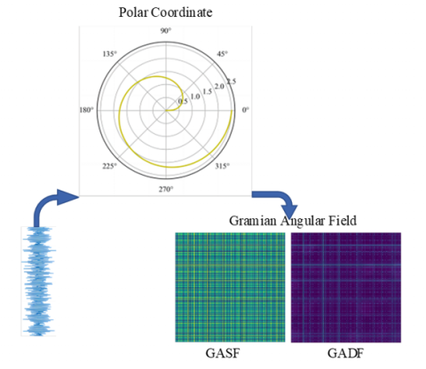
GAF [28] is able to transform one-dimensional time series data into two-dimensional image data by encoding the time series signal in the polar coordinate system, and converting the time and amplitude corresponding to the one-dimensional time series points into the radius and angles in the polar coordinate system, while maintaining time dependence.
For timing data with n points $X=\left\{x_1, x_2, \cdots, x_n\right\}$, the specific steps for GAF conversion of timing data with points are as follows:
Step 1: Normalize the time series signal, compress the value of one-dimensional data to $[-1,1]$ area.
$\tilde{x}_i=\frac{\left[x_i-X_{\max }\right]+\left[x_i-X_{\min }\right]}{X_{\max }-X_{\min }}$ (11)
$\tilde{x}_i$ for the converted $X$.
Step 2: Convert the polar coordinates of the processed sequence.
$\left\{\begin{array}{cc}\varphi=\arccos \left(\widetilde{x}_{\imath}\right) & \left(-1 \leqslant \widetilde{x}_i \leqslant 1\right) \\ r=\frac{t_i}{N} & \left(t_i \in N\right)\end{array}\right.$ (12)
where, $t_i$ denotes the timestamp of the point $x_i, N$ is a constant factor used to normalize the scale span of the polar coordinate system, and $\varphi$ denotes the angular cosine polar coordinates.
Step 3: Calculate the trigonometric sum of each polar coordinate in the system to identify the correlation between different time intervals, encode it into the geometric structure of the matrix, defined as:
$\begin{aligned} & G A F=G A S F=\left[\cos \left(\phi_i+\phi_j\right)\right] =\tilde{X}^{\prime} \cdot \tilde{X}-\sqrt{I-\tilde{X}^{\prime 2}} \cdot \sqrt{I-\tilde{X}^2}\end{aligned}$ (13)
$\begin{aligned} & G A F=G A D F=\left[\sin \left(\phi_i-\phi_j\right)\right] =\sqrt{I-\tilde{X}^{\prime 2}} \cdot \tilde{X}-X^{\prime} \sqrt{I-\tilde{X}^2}\end{aligned}$ (14)
where, $I=[1,1,1,1]$ is the unit row vector, $X$ and $X^{\prime}$ are different row vectors.
The conversion process is shown in Figure 1, GADF [29] is better than GASF in terms of image color, cross boundary and detail portrayal, and the literature [30] also shows that the recognition accuracy of extracted features using GADF is higher than that of GASF, so GADF is used for encoding in this paper.
Figure 1. Encoding process of Gram's corner field
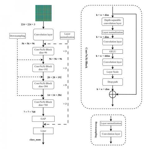
2.4 ConvNeXt module
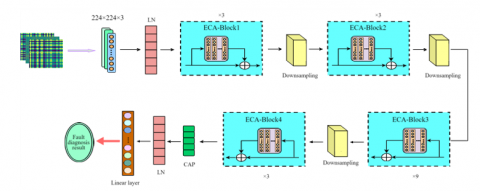
ConvNeXt algorithm [31] is improved on the basis of Residual Neural Network by referring to the idea of Swin Transformer [32], which mainly includes increasing the stacking times of a single module and using deep separable convolution instead of ordinary convolution, using7*7convolution kernel instead of 3*3convolution kernel, the Gaussian Error Linear Unit (GELU) activation function is adopted, replacing the original nonlinear activation function and batch normalization layer in ResNet, and design improvements such as...ign of inverted bottleneck layer is adopted for each block. It not only retains the advantages of traditional convolution, but also avoids the shortcomings of Transformer and improves in performance. Its structure is shown in Figure 2. In the figure, h, w, dim represent the height, width and dimension of the feature map respectively, Layer Scale is used to scale the inputs to normalize the outputs between the layers, and Drop Path is used to change the output of the main structure to 0 with a certain probability, which is equivalent to the fact that only the shortcut branch constitutes the output to prevent overfitting.
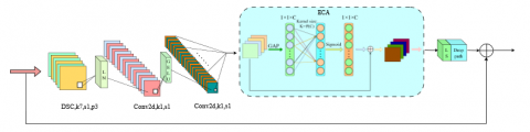
2.5 ECA module
Attention mechanism can make the model focus on important features through parameter updating, so as to fulfill the response task efficiently and accurately. Attention mechanisms are widely used in various fields, among which the commonly used ones are SE-Net, ECA-Net, SK-Net and CBAM, etc. Among them, the core idea of ECA is to compute attention in the channel dimension. Compared with other attention mechanisms, ECA, with its Event-Condition-Action rules, has been proven to be more efficient in data integration, easier to optimize for various business processes, and widely applicable across different enterprise scenarios.
In this paper, we choose ECA [33] to design ECA-Block module on the basis of Block in ConvNeXt, and the specific structure is shown in Figure 3. The ECA module is put into the original Block structure before the Drop path layer, and it can embed the positional attention information to each channel of the image, and the improved network is named as ECA-ConvNeXt.
GAP in Figure 3 denotes global average pooling, and the channel weights are generated by a one-dimensional convolutional kernel of size K. K is then determined adaptively as a function of the channel dimension C, as shown in Eq. (12), where γ = 2 and b = 1.
$k=\varphi(c)\left|\frac{\log _2(C)}{\gamma}+\frac{b}{\gamma}\right|$ (15)
Figure 2. The ConvNeXt structure
Figure 3. ECA-Block structure
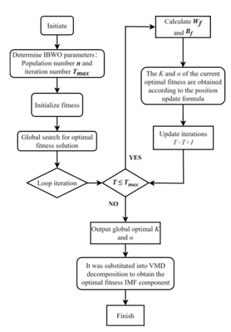
3.1 BWO-VMD
The VMD parameters are optimized by BWO to search for the optimal parameter combinations of VMD and select the optimal IMF components. The specific flowchart is shown in Figure 4, and the specific steps are as follows:
Step 1: Initialize the beluga population size, maximum number of iterations, dimensions, and search ranges for upper and lower boundaries.
Step 2: Define the fitness function, the fitness function selected in this paper is the arrangement entropy, and the value of the arrangement entropy of each IMF component is sorted. Select the current optimal fitness value.
Figure 4. BWO-VMD flow chart
Step 3: Start the global iterative search, determine the stage of beluga whales according to the values of $B f$ and $W_f$, and update the position of beluga whales population according to Eqs.(7)-(9).
Step 4: After updating the position of beluga whale population, we will calculate the fitness value again, compare the fitness value before and after updating, and keep the optimal fitness value to continue updating.
Step 5: determine whether BWO reaches the maximum number of iterations, if it reaches the maximum number of iterations, then end the loop.
Step 6: Output the optimal fitness value and the corresponding parameters K and α when the optimal fitness value is reached back into the VMD to find the IMF component of the optimal fitness.
3.2 ECA-ConvNeXt network
The enhancement of the ConvNeXt network in this paper is achieved by substituting the block in the original ConvNeXt with an ECA-Block. The model structure is illustrated in Figure 5, and the specific parameter information of the enhanced ECA-ConvNeXt network is presented in Table 1. The network model has been shown to capture spatial correlations among features across different image channels and establish long-term dependencies. This enables the model to focus its attention more precisely on fault features, resulting in enhanced performance. The model has been demonstrated to possess both generalization ability and anti-noise performance that surpass those of the common model.
Figure 5. Structure of the ECA-ConvNeXt network
Table 1. Parameters of the layers for improving ConvNeXt
|
Framework |
Importation |
Convolution Kernel and Step Size |
Exports |
|
|
224 × 224 × 3 |
4 × 4, s4 |
56 × 56 × 96 |
|
Convolutional layer 1 |
56 × 56 × 96 |
d7 × 7, s1 |
56 × 56 × 96 |
|
ECA-Block1 |
56 ×56 × 96 |
1 × 1, s1 |
56 × 56 × 384 |
|
56 × 56 × 384 |
1 × 1, s1 |
56 × 56 × 96 |
|
|
56 × 56 × 96 |
2 × 2, s2 |
28 × 28 × 192 |
|
|
Downsampling |
28 × 28 × 192 |
d7 × 7, s1 |
28 × 28 × 192 |
|
ECA-Block2 |
28 × 28 × 192 |
1 × 1, s1 |
28 × 28 × 768 |
|
28 × 28 × 768 |
1 × 1, s1 |
28 × 28 × 192 |
|
|
28 × 28 × 192 |
2 × 2, s2 |
14 × 14 × 384 |
|
|
Downsampling |
14 × 14 × 384 |
d7 × 7, s1 |
14 × 14 × 384 |
|
ECA-Block3 |
14 × 14 × 384 |
1 × 1, s1 |
14 × 14 × 1536 |
|
14 × 14 × 1536 |
1 × 1, s1 |
14 × 14 × 384 |
|
|
14 × 14 × 384 |
2 × 2, s2 |
7 × 7 × 768 |
|
|
Downsampling |
7 × 7 × 768 |
d7 × 7, s1 |
7 × 7 × 768 |
|
ECA-Block4 |
7 × 7 × 768 |
1 × 1, s1 |
7 × 7 × 3072 |
|
7 × 7 × 3072 |
1 × 1, s1 |
7 × 7 × 768 |
3.3 Network fault diagnosis based on BWO-VMD with ConvNeXt improvement
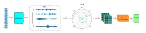
Combining the BWO-VMD feature extraction and ECA-ConvNeXt network, a bearing fault diagnosis method based on BWO-VMD and ECA-ConvNeXt is proposed, and the overall algorithm flow is shown in Figure 6, with the following specific steps:
Step 1: Decompose the bearing vibration signals of multiple fault categories using the BWO-VMD method to obtain the optimal feature IMF components.
Step 2: The IMF component is used as the feature sample of the vibration signal, and overlapping window segmentation is used to obtain multiple samples to form a data set, and the samples are converted to 2D image features by GADF.
Step 3: Divide the training samples into training set and test set, input them into ECA-ConvNext network for fault recognition training, and test them on the test set.
Figure 6. Bearing fault diagnosis flow diagram in this paper
4.1 Experimental data set
Experiments conducted at Case Western Reserve University utilize the SKF bearing data set for fault diagnosis research [34]. The dataset employs EDM to establish single-point damage faults in the ball, outer race, and inner race. Each fault type is divided into three sizes: 0.007 in, 0.014 in, and 0.021 in (1 in = 2.54 cm), and the loads of 0HP, 1HP, 2HP, and 3HP are collected under different operating conditions at 12 kHz and 48 kHz sampling frequencies at the drive and fan ends, respectively. The data were collected and analysed on the drive and fan sides under four different operating conditions, namely 0HP, 1HP, 2HP, and 3HP, at sampling frequencies of 12 kHz and 48 kHz, respectively.
4.2 Fault classification experiments based on BWO-VMD and ECA-ConvNeXt models
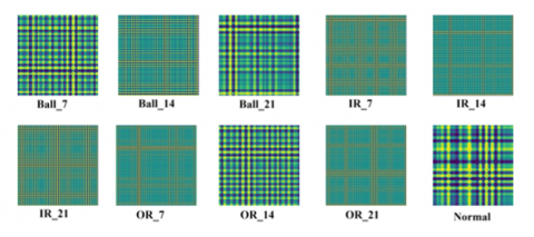
In order to ascertain the efficacy of the proposed bearing fault diagnosis model, which integrates BWO-VMD and ECA-ConvNeXt techniques, the study constructs a comprehensive dataset comprising nine distinct groups of bearing fault vibration data and one set of normal data in Table 2, all sampled at the drive end under 0HP and 12 kHz conditions. This approach facilitates simultaneous classification of both fault type and fault severity, thereby offering a more comprehensive classification scheme in comparison to that presented in previous literature [35]. However, the simultaneous classification of fault types and fault degrees may potentially compromise the algorithm's accuracy, given the ambiguity surrounding the boundaries of faults of different degrees within a given category. A comparison was made between the BWO-VMD method and NON-VMD (BWO-VMD not used) on the data set. Meanwhile, the fault diagnosis network was adopted by ECA-ConvNext, while ConvNext, ResNet, and 1D-CNN were used as four network models for control experiments. Prior to the training of the network models, the number of training and test sets was determined, with the ratio of these sets being divided at a rate of 4:1.
Table 2. Data table of experimental samples
|
Fault Type |
Fault Location |
Training Sets/Each |
Test Sets/Each |
Fault Diameter/mm |
Table |
|
Ball_7 |
Ball |
3600 |
900 |
0.007 |
0 |
|
Ball_14 |
Ball |
3600 |
900 |
0.014 |
1 |
|
Ball_21 |
Ball |
3600 |
900 |
0.021 |
2 |
|
IR_7 |
Inner race |
3600 |
900 |
0.007 |
3 |
|
IR_14 |
Inner race |
3600 |
900 |
0.014 |
4 |
|
IR_21 |
Inner race |
3600 |
900 |
0.021 |
5 |
|
Normal |
- |
3600 |
900 |
- |
6 |
|
OR_7 |
Outer race |
3600 |
900 |
0.007 |
7 |
|
OR_14 |
Outer race |
3600 |
900 |
0.014 |
8 |
|
OR_21 |
Outer race |
3600 |
900 |
0.021 |
9 |
4.2.1 Preprocessing of the BWO-VMD dataset
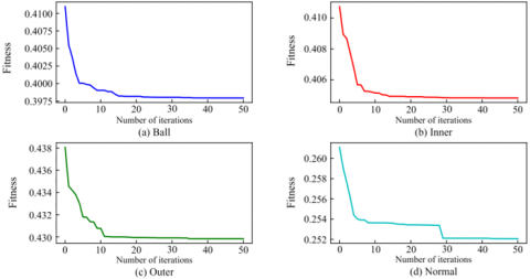
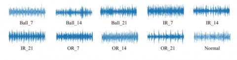
The original vibration signal is firstly processed by the BWO-VMD method, and the IMF components are extracted as the sample features, and the BWO parameter settings are shown in Table 3. With the 7 mm radius as the representative of various types of fault features, the iterative graph of the BWO-VMD adaptivity is shown in Figure 7, which has basically converged after 30 iterations, and the overall convergence speed is faster, and the processed IMF components are shown in Figure 8. The processed IMF component is shown in Figure 8. The processed one-dimensional data is partitioned, and each 1024 points is taken as a sample, and there are 4500 samples for each fault type. Each sample is converted to image features using the GADF method as shown in Figure 9. The image size for GADF conversion is set to 256 × 256.
Table 3. BWO parameter settings
|
n |
T |
d |
m |
K |
α |
|
20 |
50 |
2 |
5 |
[3, 10] |
[200, 2000] |
Figure 7. Iterative plot of BWO-VMD adaptation
Figure 8. Vibration signal after BWO-VMD decomposition
Figure 9. GAF encoded image
4.2.2 Algorithm model parameterization
ECA-ConvNext and ConvNext, ResNet and 1D-CNN four network models for fault diagnosis classification experiments, algorithm model based on the Pytorch deep learning framework implementation, the operating environment for Python3.8, Pytorch1.12, CUDA11.3, the number of training iterations of the four models Epoch is set at 150, Batch_Size is set to 16, for ConvNeXt network choose AdamW (Adam with Weight Decay Fix) optimizer to update the network parameters, for ResNet network choose Aadm optimizer, the learning rate is set to 0.003. Loss function choose cross entropy, network input image size is 224 × 224.
4.2.3 Analysis of experimental results of algorithmic model fault classification
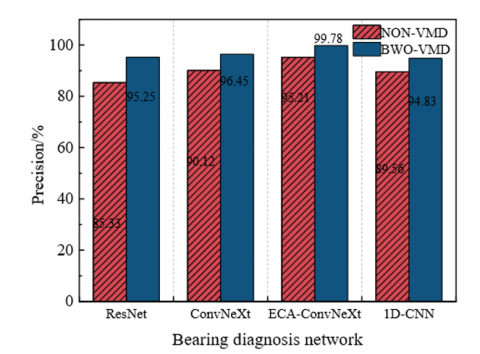
Four kinds of network models are employed to carry out fault diagnosis classification experiments on the features extracted by the BWO-VMD method and the features extracted by the NON-VMD method (which means that the BWO-VMD is not used), respectively, and the experimental results are shown in Figure 10. As is evident from the figure, under the same recognition classification network model, the classification accuracy of the bearing fault classification experiments on the features extracted by the BWO-VMD method is higher than that of the NON-VMD method. This indicates that the BWO-VMD method can effectively extract the signal fault features and verifies the effectiveness of the BWO-VMD method. Conversely, irrespective of the adoption of the BWO-VMD method, the ECA-ConvNeXt model in this paper exhibits superior performance in terms of fault diagnosis classification accuracy when compared with the native ConvNeXt network and the other two types of networks. The study reports an accuracy of 99.78% for fault identification when employing the BWO-VMD with the ECA-ConvNeXt model.
Figure 10. Comparison of different diagnostic methods with different loads
4.3 Variable operating condition experiments based on BWO-VMD and ECA-ConvNeXt algorithm models
The device exhibits varying working conditions based on different loads across diverse scenarios. If a model trained under a specific load condition still demonstrates a superior recognition effect under other load conditions, this signifies that the model possesses strong generalisation ability and robustness, thereby enhancing its practical application value [36]. In order to verify the generalization performance of the model in this paper, the data under the loads of 0HP, 1HP, and 2HP in the CWRU dataset are used as three datasets of A(0HP), B(1HP), and C(2 HP) are selected two at a time, one of them as the training set, and one of them as the test set, and multiple crossover experiments are carried out to test the algorithmic model by adopting the same preprocessing and parameter settings as those in Section 3.2. The same preprocessing and parameter settings as in Section 3.2 were used to test the migration robustness of the algorithmic model under variable operating conditions (variable load).
The performance of the four algorithms across various training and test set combinations, as depicted in Table 4, reflects the importance of proper data set division in machine learning. The performance of the algorithms is measured by the mean and standard deviation of the recognition rate of the same algorithmic model on six combinations. The average recognition rate reflects the performance of the algorithms, and the standard deviation of the recognition rate reflects the fluctuation of the algorithmic performance in the migration experiments. Smaller fault indications show that the algorithms have enhanced robustness, with the ECA-ConvNeXt achieving optimal performance across six variable working condition (load) scenarios. The ConvNeXt model demonstrates optimal performance in six distinct variable working condition (load) scenarios, exhibiting an average recognition rate of 96.22%, which is significantly higher than the performance of the other algorithms. The standard deviation of the ConvNeXt model is 3.4. The experimental results demonstrate that the ECA-ConvNeXt model of this paper exhibits superior adaptability in variable working conditions, i.e., it demonstrates enhanced robustness.
Table 4. Experimental results of four algorithms modeling working condition migration
|
Training Set/Test Set Diagnostic Network |
A→B |
A→C |
B→A |
B→C |
C→A |
C→B |
Average Value/% |
Standard Deviation/% |
|
ResNet |
80.02 |
83.15 |
73.4 |
71.29 |
78.38 |
69.53 |
75.96 |
5.36 |
|
ConvNeXt |
82.23 |
82.18 |
72.11 |
76.84 |
77.23 |
78.22 |
78.13 |
3.79 |
|
ECA-ConvNeXt |
98.19 |
94.27 |
97.86 |
97.81 |
90.13 |
99.07 |
96.22 |
3.41 |
|
1D-CNN |
86.78 |
82.16 |
86.44 |
81.91 |
76.32 |
80.5 |
82.35 |
3.91 |
4.4 Experiments on model noise immunity based on BWO-VMD and ECA-ConvNeXt algorithms
4.4.1 Noise test data
The CWRU dataset is collected in an experimental environment with weak background noise, and the noise may be larger in practical applications, so Gaussian white noise with different signal-to-noise ratios is added to the experimental data to simulate the real operating scenarios to further validate the model performance. By introducing noise into the original signal, the distinctive features of bearing faults become obscured, there by heightening the challenges associated with fault diagnosis. In order to verify the robustness of the model under noisy conditions,rify the effectiveness of the algorithm in a noisy environment, noise is added to the original Normal data with 0HP load to generate noisy signals of 0dB, -4dB and -8dB as new data sets for algorithm performance testing. The performance of the algorithm is tested on the original Normal data with 0HP load.
Signal-to-Noise Ratio (SNR) is a critical indicator of the quality of a signal, quantifying the level of noise present within it. It is calculated using the formula SNR = 10 * log10(Ps/Pn), where Ps represents the power of the signal and Pn the power of the noise.
$S N R_{d B}=10 \log \frac{P_{\text {signal }}}{P_{\text {noise }}}$ (16)
where, $P_{\text {signal }}$ is the signal power, and $P_{\text {noise }}$ is the noise power. The larger the SNR value, the smaller the proportion of noise.
Table 5. Results of four algorithms on different noise datasets (%)
|
Signal-to-noise Ratio (dB) Diagnostic Network |
Normal |
0 |
-4 |
-8 |
|
ResNet |
95.25 |
92.14 |
92.27 |
90.50 |
|
ConvNeXt |
96.45 |
92.03 |
92.24 |
91.71 |
|
ECA-ConvNeXt |
99.89 |
99.68 |
99.57 |
99.78 |
|
1D-CNN |
94.83 |
85.71 |
85.35 |
87.46 |
4.4.2 Trouble shooting experiments with signal loading noise
Initially, BWO-VMD features were extracted for normal, 0 dB, -4 dB and -8 dB noise datasets. Subsequently, classification and recognition tests for fault diagnosis were conducted using ECA-ConvNeXt, ConvNeXt, ResNet and 1DCNN models, and the results are shown in Table 5. In the data set characterised by varying signal-to-noise ratios, the model proposed in this study exhibited superior accuracy, attaining a minimum of 99.57% and a maximum of 99.89% in terms of correctness, thereby surpassing the performance of the other four models.The recognition rate following the introduction of noise remained largely unaltered in comparison to the unloaded noise Normal data, while the recognition rate of the aforementioned three models underwent a more substantial decline, thereby signifying that the algorithm model presented in this study demonstrates remarkable resilience to noise.
4.4.3 Analysis of model migration results for signal loaded noise
In practical applications, the signal-to-noise ratio of collected signals may vary depending on changes in the working condition of the same device, as well as differences in working scenes for the same device. A model that maintains superior recognition performance across varying signal-to-noise ratios demonstrates enhanced generalization capabilities and robustness., which has a better value for practical applications.
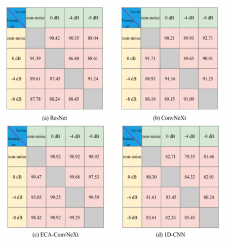
In order to verify the migration effect of the algorithmic model in different working conditions (noise), the noise migration experiments of the algorithmic model were conducted with the original Normal dataset with 0HP load and the noise-enhanced datasets formed by adding noise at 0dB, -4dB, and -8dB to it, four datasets in total, and one dataset was selected as the training set, and the other three datasets with different SNR were used as the test set, and the ECA-ConvNeXt, ConvNeXt, ResNet, a1DCNN algorithmic models were cross-trained and tested with 12 datasets. ECA-ConvNeXt, ConvNeXt, ResNet, and 1DCNN were used for cross-training and testing, with recognition accuracies for each model migrating between different noisy datasets shown in Figure 11. The vertical axis of Figure 11 represents the recognition accuracy of the trained network model under the training set. network model under the test dataset in the horizontal axis. The data in the figure shows that the recognition accuracy of the trained network model on the training set is located in the vertical axis, while the recognition accuracy of the network model on the test data set is located in the horizontal axis. The mean and standard deviation of the correct recognition rates of 12 sets of migration experiments of the four algorithm models are shown in Table 6.
Figure 11. Experimental results of network migration between loaded noisy datasets
Table 6. Statistics of experimental results on model noise transfer
|
|
ResNet |
ConvNeXt |
ECA-ConvNeXt |
1D-CNN |
|
Average recognition rate/% |
89.00 |
90.33 |
98.83 |
82.23 |
|
Recognition rate standard deviation/% |
1.58 |
1.29 |
1.24 |
1.79 |
As can be seen in Figure 11 and Table 6, in the migration test experiments on the original dataset and the new dataset composed of loaded white noise with different signal-to-noise ratios, the bearing diagnostic model based on BWO-VMD and ECA-ConvNeXt has an average correct rate of fault diagnosis identification of 98.83% in the 12 sets of tests, and the optimal rate is 99.92%, which is much higher than that of the other three algorithmic models. At the same time, the standard deviation of the corThe error rate of this algorithm model in the migration test among 12 different data sets is also the lowest among the four algorithm models, which is 1.24%. The standard deviation of its accuracy rate is also the smallest among the four, which is 1.24%. That is to say, the fluctuation of this model is the smallest in the migration test among different noisy datasets, which indicates that this algorithm model has the best anti-noise ability and robustness under the noise environment.
To enhance the precision and reliability of rolling bearing fault identification, a novel methodology for diagnosing bearing faults is presented in this paper. This methodology employs a combination of BWO-VMD and ECA-ConvNeXt algorithms. The following conclusions are drawn:
1) This paper employs BWO-VMD to decompose bearing vibration signals and select optimal IMF components, converting 1D features to 2D images via GADF. By integrating a channel attention mechanism (ECA) into ConvNeXt, it enhances feature focus, significantly improving fault recognition accuracy and robustness.
2) The BWO-VMD algorithm significantly enhances fault feature extraction, effectively improving fault identification and classification accuracy across multiple network models.
3) The integration of ECA-ConvNeXt and BWO-VMD significantly enhances noise resistance and fault recognition accuracy reaching 99.57%. In migration experiments, average recognition rates under load and noise variations reached 96.22% and 98.22% respectively, surpassing comparative algorithms with minimal standard deviation, demonstrating exceptional robustness and generalization capability.
The employment of the IMF component that exhibits the minimum arrangement entropy, decomposed through the BWO-VMD algorithm, is a distinctive feature of this paper. Future research endeavors will focus on harnessing additional information from the IMF component and integrating multi-channel information to leverage the channel attention mechanism effectively.
This thesis is supported by the key project of the National Natural Science Foundation of China, “Intelligent diagnosis, prediction, and maintenance of abnormal conditions in large petrochemical plants” (Grant No.: 61933013) and Natural Science Foundation of the Higher Education Institutions of Guangdong Province (Grant No.: 2020KTSCX083) and the Science and Technology Program of Maoming (Grant No.: 2021KJZXZ1GSPDX001).
[1] Xiao, C., Chang, J., Yu, J. (2025). Multiple wave-shape mode decomposition for bearing fault diagnosis. IEEE Transactions on Instrumentation and Measurement, 74: 6507811. https://doi.org/10.1109/TIM.2025.3588996
[2] Ren, Y., Li, W., Luan, F., Yuan, S. (2025). A domain adaptation method based on improved cycle-GAN for Zero-shot fault diagnosis. IEEE Sensors Journal, 25(17): 32282-32292. https://doi.org/10.1109/JSEN.2025.3589457
[3] Nguyen, T.D., Pham, T.T., Phuc, T.L., Nguyen, P.D. (2025). Spectrogram zeros method for rolling bearing fault diagnosis under variable rotating speeds. IEEE Access, 13: 108862-108872. https://doi.org/10.1109/ACCESS.2025.3582280
[4] Liu, Q., Yang, J., Zhang, K. (2022). An improved empirical wavelet transform and sensitive components selecting method for bearing fault. Measurement, 187: 110348. https://doi.org/10.1016/j.measurement.2021.110348
[5] Tomar, A.S., Jayaswal, P. (2024). Rolling element bearing fault investigation based on translation invariant wavelet means denoising and empirical mode decomposition (EMD). Journal of The Institution of Engineers (India): Series C, 105(1): 127-140. https://doi.org/10.1007/s40032-023-01016-w
[6] Ye, X., Hu, Y., Shen, J., Feng, R., Zhai, G. (2020). An improved empirical mode decomposition based on adaptive weighted rational quartic spline for rolling bearing fault diagnosis. IEEE Access, 8: 123813-123827. https://doi.org/10.1109/ACCESS.2020.3006030
[7] Hou, J., Wu, Y., Gong, H., Ahmad, A.S., Liu, L. (2020). A novel intelligent method for bearing fault diagnosis based on EEMD permutation entropy and GG clustering. Applied Sciences, 10(1): 386. https://doi.org/10.3390/app10010386
[8] Chang, B., Zhao, X., Guo, D., Zhao, S., Fei, J. (2024). Rolling bearing fault diagnosis based on optimized VMD and SSAE. IEEE Access, 12: 130746-130762. https://doi.org/10.1109/ACCESS.2024.3386835
[9] Ma, Z., Zhang, Y. (2025). A study on rolling bearing fault diagnosis using RIME-VMD. Scientific Reports, 15(1): 4712. https://doi.org/10.1038/s41598-025-89161-3
[10] Wang, Z., Xu, Z., Cai, C., Wang, X., et al. (2024). Rolling bearing fault diagnosis method using time-frequency information integration and multi-scale TransFusion network. Knowledge-Based Systems, 284: 111344. https://doi.org/10.1016/j.knosys.2023.111344
[11] Yu, S., Liu, H., Zhu, H., Hu, K., Liu, Y. (2024). Rolling bearing fault analysis based on variational mode decomposition and multiscale arrangement entropy. Journal of Vibroengineering, 26(6): 1301-1316. https://doi.org/10.21595/jve.2024.23912
[12] Wang, H., Li, Y., Zhao, Y. (2021). Application of denoising method of k-value optimized VMD combined with wavelet packet analysis in tunnel blasting signal. Explos. Mater, 50(5): 50-57.
[13] He, Y., Wang, H., Gu, S. (2021). New fault diagnosis approach for bearings based on parameter optimized VMD and genetic algorithm. Journal of Vibration and Shock, 40(6): 184-189.
[14] Li, H., Liu, T., Wu, X., Chen, Q. (2020). An optimized VMD method and its applications in bearing fault diagnosis. Measurement, 166: 108185. https://doi.org/10.1016/j.measurement.2020.108185
[15] Gao, H., Zhang, X., Gao, X., Li, F., Han, H. (2024). Multi-timescale attention residual shrinkage network with adaptive global-local denoising for rolling-bearing fault diagnosis. Knowledge-Based Systems, 304: 112478. https://doi.org/10.1016/j.knosys.2024.112478
[16] Zhou, J., Xiao, M., Niu, Y., Ji, G. (2022). Rolling bearing fault diagnosis based on WGWOA-VMD-SVM. Sensors, 22(16): 6281. https://doi.org/10.3390/s22166281
[17] Wang, T., Khoo, S.Y., Ong, Z.C., Siow, P.Y., Wang, T. (2025). Distance similarity entropy: A sensitive nonlinear feature extraction method for rolling bearing fault diagnosis. Reliability Engineering & System Safety, 255: 110643. https://doi.org/10.1016/j.ress.2024.110643
[18] Zhang, L.M., Chao, W.W., Liu, Z.Y., Cong, Y., Wang, Z.Q. (2022). Crack propagation characteristics during progressive failure of circular tunnels and the early warning thereof based on multi-sensor data fusion. Geomechanics and Geophysics for Geo-Energy and Geo-Resources, 8: 172. https://doi.org/10.1007/s40948-022-00482-3
[19] Li, C., Zhang, S., Qin, Y., Estupinan, E. (2020). A systematic review of deep transfer learning for machinery fault diagnosis. Neurocomputing, 407: 121-135. https://doi.org/10.1016/j.neucom.2020.04.045
[20] Wang, H., Liu, C., Du, W., Wang, S. (2021). Intelligent diagnosis of rotating machinery based on optimized adaptive learning dictionary and 1DCNN. Applied Sciences, 11(23): 11325. https://doi.org/10.3390/app112311325
[21] Wang, H., Liu, Z., Peng, D., Qin, Y. (2019). Understanding and learning discriminant features based on multiattention 1DCNN for wheelset bearing fault diagnosis. IEEE Transactions on Industrial Informatics, 16(9): 5735-5745. https://doi.org/10.1109/TII.2019.2955540
[22] Zhang, Y., Xing, K., Bai, R., Sun, D., Meng, Z. (2020). An enhanced convolutional neural network for bearing fault diagnosis based on time–frequency image. Measurement, 157: 107667. https://doi.org/10.1016/j.measurement.2020.107667
[23] Zhao, B., Zhang, X., Li, H., Yang, Z. (2020). Intelligent fault diagnosis of rolling bearings based on normalized CNN considering data imbalance and variable working conditions. Knowledge-Based Systems, 199: 105971. https://doi.org/10.1016/j.knosys.2020.105971
[24] Zhao, Y., Tang, W.S., Nie, Y.H., Wang, Z.T. (2022). Broadband oscillation classification method based on GADF-AlexNet. Power System Technology, 11: 4364-4372.
[25] Wan, K., Ma, H., Cui, J., Wang, J. (2023). Fault diagnosis method of transformer core loosening based on Mel-GADF and ConvNeXt-T. Electric Power Automation Equipment, 44(3): 217-224. https://doi.org/10.16081/j.epae.202307003
[26] Guo, J, Hao, G., Li, X., Yu, J., Hu, Z. (2025). Threshold variational mode decomposition cascade high concentrated time–frequency analysis algorithm. Mechanical Systems and Signal Processing, 239: 113337. https://doi.org/10.1016/j.ymssp.2025.113337
[27] Zhao, Z., Liu, C., Wang, J., Luo, J., et al. (2025). Intelligent optimization control of plate plan-view pattern based on intermediate slab pattern vision inspection and BWO-DNN algorithm. Materials, 18(13): 3038. https://doi.org/10.3390/ma18133038
[28] Zhong, C., Li, G., Meng, Z. (2022). Beluga whale optimization: A novel nature-inspired metaheuristic algorithm. Knowledge-based Systems, 251: 109215. https://doi.org/10.1016/j.knosys.2022.109215
[29] Wang, P., Song, Y., Wang, X., Guo, X., Xiang, Q. (2025). ImagTIDS: An internet of things intrusion detection framework utilizing GADF imaging encoding and improved transformer. Complex & Intelligent Systems, 11(1): 93. https://doi.org/10.1007/s40747-024-01712-9
[30] Hou, D.X., Mu, J.T., Fang, C., Shi, P.M. (2022). Fault diagnosis of variable speed bearings based on GADF and ResNet34 introduced transfer learning. Journal of Northeastern University (Natural Science), 43(3): 383. https://doi.org/10.12068/j.issn.1005-3026.2022.03.011
[31] Liang, H., Cao, J., Zhao, X. (2023). Small sample fault diagnosis method for rotating machinery based on GADF and PAM-resnet. Control and Decision, 38(12): 3465-3472.
[32] Li, M., Qin, J., Li, D., Chen, R., Liao, X., Guo, B. (2021). VNLSTM-PoseNet: A novel deep ConvNet for real-time 6-DOF camera relocalization in urban streets. Geo-Spatial Information Science, 24(3): 422-437. https://doi.org/10.1080/10095020.2021.1960779
[33] Xu, Y., Qiao, X., Ding, L., Li, X., Chen, Z., Yue, X. (2025). Enhanced YOLOv5 with ECA module for vision-based apple harvesting using a 6-DOf robotic arm in occluded environments. Agriculture, 15(17): 1850. https://doi.org/10.3390/agriculture15171850
[34] Wang, Q., Wu, B., Zhu, P., Li, P., Zuo, W., Hu, Q. (2020). ECA-Net: Efficient channel attention for deep convolutional neural networks. In 2020 IEEE/CVF Conference on Computer Vision and Pattern Recognition (CVPR), Seattle, WA, USA, pp. 11531-11539. https://doi.org/10.1109/CVPR42600.2020.01155
[35] Zhang, X., Zhao, B., Lin, Y. (2021). Machine learning based bearing fault diagnosis using the case western reserve university data: A review. IEEE Access, 9: 155598-155608. https://doi.org/10.1109/ACCESS.2021.3128669
[36] Su, S., Zhang, Z. (2023). Bearing fault diagnosis method based on HCDDP. Journal of Vibration and Shock, 42(23): 103-111. https://doi.org/10.13465/j.cnki.jvs.2023.23.013