Junmin Xue![]() | Yunbo Rao*
| Yunbo Rao*![]() | Qingsong Lv
| Qingsong Lv![]() | Qinwei Yao
| Qinwei Yao![]() | Cheng Huang
| Cheng Huang![]() | Jiafu Su
| Jiafu Su![]()
© 2025 The authors. This article is published by IIETA and is licensed under the CC BY 4.0 license (http://creativecommons.org/licenses/by/4.0/).
OPEN ACCESS
Kidney tumor segmentation from CT images remains a challenging task due to the presence of noise, indistinct boundaries, diminished contrast, and varying morphological characteristics between the kidney and tumor. Most existing methods rely on the Softmax function to generate pixel-wise class probabilities and segmentation outcomes, but this approach has limitations in accurately delineating pixels with ill-defined edges. To overcome this problem, we propose a novel Edge-Refine Network (ERNet) that refines the Softmax-based pixel attributions to achieve precise segmentation of kidney tumors. ERNet leverages the Segmentation via Gradient-weighted Class Activation Mapping (Seg-Grad-CAM), a novel technique that produces interpretable heatmaps that highlight the pixels that are difficult to segment. By using backpropagation, ERNet retrains the model with the heatmap weights and the target probabilities from the Softmax function, thereby enhancing the segmentation accuracy. We evaluate our method on publicly available kidney tumor datasets and show that ERNet outperforms the state-of-the-art methods in kidney tumor segmentation, achieving a 2.9% improvement in the Dice score and a 4.17% reduction in the ASD. Moreover, ERNet exhibits superior precision in segmenting intricate details, especially in regions with ambiguous boundaries.
kidney tumor segmentation, blurry boundaries, interpretable heatmaps, Edge Refine Network
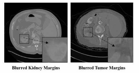
Early and accurate identification of kidney cancer is crucial for improving the survival rate of patients, as the tumor can spread to nearby tissues or organs and increase the mortality risk. However, diagnosing kidney cancer has been a challenging task for the past decade [1]. Clinical practice faces difficulties due to the noise in CT images, which causes blurry boundaries, low contrast, and varying morphological features between the kidney and the tumor, as shown in Figure 1. Therefore, detecting and segmenting the kidney and tumor accurately are major challenges. Organ and tumor segmentation are important but difficult problems in medical imaging [2]. Manual segmentation of the kidney is especially time-consuming and labor-intensive, and often leads to inconsistent results. Radiologists spend a lot of time processing numerous CT images [3].
Furthermore, extracting kidney features accurately depends on capturing the intensity variations among the voxels near the kidney boundary in CT images [4]. However, the presence of blurred voxels around the organ boundary complicates the task [5]. Moreover, the texture similarity between tumors and the kidney poses a challenge for the identification process [6]. Nevertheless, precise delineation of kidney tumors is vital for preoperative evaluation and surgical planning.
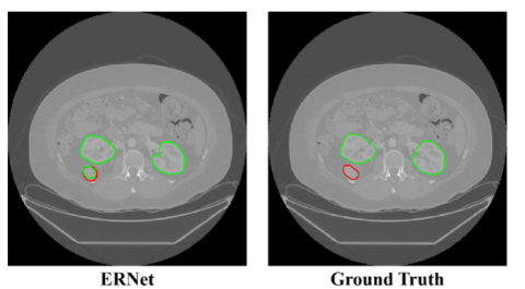
Figure 1. Kidney and Tumor Segmentation. Left: segmentation results generated by ERNet. Right: corresponding ground truth, where the tumor is annotated as part of the kidney
Various methods have been proposed to achieve precise segmentation of kidney tumors. Thresholding segmentation and its variants are often preferred by researchers as the primary techniques for segmenting the target [7]. For example, one method divides the global image segmentation task into local tasks, applies thresholding segmentation to each block, and then clusters the blocks to identify the target region [8]. Another method combines K-means clustering with thresholding segmentation for kidney tumor segmentation [9]. These methods suggest that local segmentation performs better than global segmentation. However, these threshold-based methods also have limitations due to their inability to separate the overlapping regions in the grayscale image between the target and background [10].
In recent years, deep learning methods have made significant progress in medical image segmentation [11-13]. However, due to the high cost and limited availability of medical datasets, data augmentation is often required during the training process to improve the training performance. For instance, some methods use weakly supervised techniques to enlarge kidney tumor segmentation datasets [14], and some methods use neural networks to augment datasets and integrate them with designed modules for target segmentation [15]. Moreover, the Region Proposal Network (RPN) generates multiple target sub-regions for further training [16]. These approaches have all contributed to the advancement of kidney tumor segmentation. However, some studies have also highlighted the importance of dataset curation, which involves removing images or slices that do not contain the kidney region, leading to better segmentation results [17].
Numerous advanced deep learning models have been applied in the realm of kidney tumor segmentation. Noteworthy examples encompass encoder-decoder architectures such as U-Net, as well as the sophisticated DeepLab series networks and the Mask R-CNN networks, which incorporate candidate box handling to refine segmentation accuracy in medical contexts [18]. U-Net can achieve satisfactory results for kidney tumor segmentation, but it still faces difficulties in segmenting edges accurately due to their low contrast [19]. Therefore, several modified versions of U-Net have been proposed for kidney segmentation, such as combining SegNet with U-Net to enhance the global contextual information [20], incorporating attention mechanisms into U-Net with residual networks and fine-tuning with preprocessed contours [21], and achieving precise segmentation by integrating 3D point clouds with U-Net [22]. Moreover, tumor segmentation has been performed using Dense U-Net after downsampling features [23].
The DeepLab series have improved the encoder and decoder for semantic seg-mentation. For instance, the DPN-131 encoder has been combined with the DeepLab v3+2.5D model for initial segmentation, followed by post-processing [24]. These methods enhance the feature representation and extraction ability of the network, thereby increasing the probability of pixels with target features being classified correctly. The Mask R-CNN series, based on the Fast RCNN series, propose generating multiple candidate regions and then performing pixel-wise classification after locating the target regions. This approach inspires us to not only improve the feature-containing pixels during neural network feature computation, but also consider making refinements based on the final pixel classification position.
The neural network often misclassifies the low contrast and blurry edges of kidney tumors as background or other objects, as it assigns a higher probability of belonging to another class to such pixels. However, many methods suffer from the problem of blurry edges of the kidney being misclassified as background [25, 26]. Based on the principles of probability theory, the Bayes rule implies that these pixels are difficult or unable to meet the probability threshold of being classified as the target [27, 28]. Consequently, a simplistic approach relying solely on a comparison of maximum probabilities across various classes for each pixel fails to yield satisfactory results within the neural network’s final output. Instead, the probability judgment for each pixel should be revised based on probability theory. By addressing this pivotal aspect, the neural network can then recalibrate its probability assignments, fostering more accurate segmentation outcomes, particularly in scenarios marked by ambiguous edges.
The development of explainable neural networks in recent years has provided a solution to this problem. Seg-GRAD-CAM can generate a heatmap of the last convolutional layer, where the heatmap’s weight indicates the importance of that pixel for the final segmentation result, with higher weights implying greater importance, and vice versa [29]. During Seg-Grad-CAM’s experiments, the pixels with lower importance tend to have smaller heatmap weights, and these pixels often correspond to blurry edges. Therefore, with the help of interpretable heatmaps, we can identify and separate the pixels that need revision during the training process. Using neural network techniques such as BP, the network can learn the heatmap weights of pixels, the probability values of the pixel being classified as the target, and its corresponding label. This enables the network to learn the relationships between these factors and segment the edges of kidney tumors accurately.
In summary, our contributions are as follows:
(1) We propose an Edge Refine Network (ERNet) that can segment kidney tumors with low-contrast and blurry edges accurately.
(2) Based on probability theory, we introduce an approach to reset the target probabilities from the neural network’s tail to address the segmentation of images with blurry boundaries.
(3) ERNet achieves state-of-the-art segmentation performance on two publicly available kidney tumor datasets, especially excelling in segmenting images with indistinct edges.
In this section, we review three key categories of research that are closely related to our work. First, we survey the current state of segmentation methods for kidney tumors and other medical targets. Second, we examine the popularized improved methods based on Softmax. Third, we discuss the evolution of interpretable heatmaps.
2.1 Segmentation methods for kidney tumors
Many methods have been proposed to address the complex challenge of kidney tumor segmentation. One notable approach is to refine U-Net segmentation by applying selective training data sets in the input section of the neural network. The architecture of an Ensemble of U-Net Models (Ens-UNet) is carefully designed, consisting of four downsampling blocks, one feature representation block, four upsampling blocks, and a final output convolution layer [30]. Each block has two identical 3×3 convolutional layers, and each downsampling block is followed by a 2×2 max-pooling operation. In a seamless integration, a 2×2 2-D transposed convolutional layer with a stride of 2×2 is concatenated with the features from the downsampling blocks, following the core structure of U-Net [31].
Moreover, enhancing the feature representation in the intermediate stages of neural networks has shown great promise. For instance, Reverse Boundary Channel Attention (RBCA) introduces a novel and ingenious method of isolating tumor slices, enabling separate training and empowering the neural network to effectively capture and learn crucial tumor features [32]. Simultaneously, the Attention-UNet architecture refines U-Net by emphasizing regions of interest, such as the kidney and tumor, through an intelligent attention mechanism, while suppressing the influence of non-focus areas [33]. In the output section of the neural network, A triple-stage self-guided network (TSS) optimizes information retention by skillfully introducing modifications to the pooling process [34]. Similarly, a detection platform for colorectal cancer (DPC) focuses on fine-tuning the input data set, striving to achieve enhanced rectal cancer segmentation accuracy [35]. In contrast, Prostate cancer of magnetic (PCM) adopts a data set expansion strategy, propelling Mask RCNN’s segmentation performance for prostate segmentation to new heights [36]. Implementing these strategic improvements at different positions within the neural network collectively serves the overarching goal of enhancing the network’s proficiency in extracting and preserving critical features, resulting in a more robust and accurate kidney tumor segmentation model.
2.2 Improved methods based on Softmax
Segmentation accuracy depends on both the feature extraction capability of neural networks and the discriminative ability of the decision structure [37]. To refine the segmentation process, it is essential to optimize both aspects. Feature extraction enables the network to capture relevant and distinctive characteristics of the target objects, facilitating more precise segmentation. However, without a discriminative decision structure, the network may struggle to effectively distinguish between different classes, leading to misclassifications and diminished segmentation accuracy [38].
The stack Net research addresses this challenge by conducting a thorough exploration of various classifiers for automated COVID detection [39]. The research develops a stacked ensemble model comprising diverse classifiers, tailored to leverage their unique strengths and overcome individual limitations. The ensemble model collaboratively analyzes input data, combining the knowledge from multiple classifiers to arrive at a more robust and accurate segmentation output. This innovative approach demonstrates the power of collaboration in enhancing the performance of segmentation tasks, especially in applications like COVID detection.
Additionally, the Region-wise loss (RWL) method introduces a Modified Region-Aware Map, which represents a simplified adaptation of the boundary distance map [40]. This novel map takes into account not only class imbalance but also pixel importance, enabling the fine-tuning of Softmax outputs. By considering both class distribution and pixel significance, the segmentation results are substantially improved. This intelligent approach ensures that the network’s predictions are better aligned with the underlying structure of the data, leading to more accurate and reliable segmentation outcomes.
Furthermore, activations extracted from CNN (AE-CNN) pioneers a sophisticated fusion of Fourier transform and Gradient-Weighted Class Activation Mapping (Seg-Grad-CAM) techniques to process input images effectively [41]. This multi-faceted approach involves a series of steps to enrich the network’s discriminative capacity. Three distinct ResNet models generate type-based activations, harnessing the diversity of information captured by each model. Subsequently, a local interpretable model-agnostic explanation method is employed to identify the most appropriate type-based activation from the CNN model. This selective activation enables the network to focus on crucial regions relevant to segmentation targets, thus fine-tuning its decision-making process. The Softmax method is then utilized to perform reclassification based on the optimized activations, further refining the segmentation outcomes. This comprehensive strategy exemplifies the fusion of innovative techniques to empower Softmax with the capability to discriminate between different segmentation targets effectively. The result is a network that is not only proficient in recognizing and preserving key features but also excels in reconfiguring pixel representations for more accurate and refined segmentation results.
2.3 Advances in interpretable heat maps
The challenge of determining which pixels’ representations necessitate adjustment or enhancement during the training process is a complex one that the traditional Softmax approach encounters. In recent years, the concept of Class Activation Mapping (CAM) has paved the way in this regard, enabling the identification of critical regions for the classification process [42]. Building upon CAM, subsequent algorithms like Score-CAM and Ablation-CAM have evolved to delve deeper into activation maps and feature map weights, enhancing the interpretability and comprehensibility of the results [43]. Within the realm of image segmentation, innovative methods like Eigen-CAM and Layer-CAM have further refined the CAM approach. By optimizing computational branches and expanding the perceptual field through intricate features, these methods have pushed the boundaries of segmentation accuracy [44]. The culmination of these advancements, including the Seg-Grad-CAM methodology, has paved the way for pixel-level analysis of heatmaps. This, in turn, has unlocked a treasure trove of insights into the intricate processes of image segmentation. Importantly, Seg-Grad-CAM provides the theoretical foundation upon which the proposed ERNet is built, a novel approach aimed at resetting the Softmax pixel class probabilities to achieve superior segmentation outcomes.
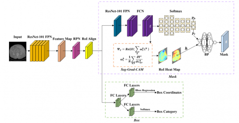
In this section, we will provide a detailed description of the implementation process of ERNet for kidney tumor segmentation. As depicted in Figure 2, the process consists of two branches: the Mask RCNN box branch for locating the Region of Interest (RoI) and the Mask branch for obtaining the mask segmentation [45]. The Mask branch comprises three steps, namely, obtaining class probabilities using Softmax, generating heatmap weight maps with Seg-Grad-CAM, and obtaining pixel segmentation results through BP fitting.
3.1 Overview of ERNet
The ERNet segmentation methodology is visually elucidated in Figure 2. The process commences with kidney tumor images being subjected to the Mask RCNN, which undertakes the computation of multiple RoIs encompassing the tumor regions while concurrently determining pixel class probabilities via Softmax activation. To ensure robust feature extraction, the ResNet-101 architecture is harnessed to generate a backbone feature pyramid that effectively captures the essence of the input images. This pyramid is subsequently subjected to RoI Align, a pivotal step that facilitates accurate alignment between RoIs and the corresponding pixel positions on the feature map, accomplished through bilinear interpolation. With the overarching objective of encompassing the tumor region to the greatest extent possible, the process employs two sub-branches—Box Coordinates and Box Category—that are instrumental in determining RoIs that optimally cover the expansive area of the kidney tumor region. The features of each pixel are channeled through the ResNet-101 backbone and the Fully Convolutional Network (FCN) to compute pixel-wise class probabilities via the Softmax mechanism. Concurrently, the Seg-Grad-CAM module comes into play, calculating interpretable heatmaps derived from the last convolutional layer within the FCN. The final steps involve fine-tuning the class probabilities derived from Softmax and the corresponding heatmap weights in conjunction with the ground truth labels. This meticulous fine-tuning process is facilitated through the application of BP fitting, a technique that optimally adjusts the model parameters to yield refined kidney tumor segmentation results of the highest precision and accuracy. In the subsequent sections, we will delve into a detailed exploration of the pivotal components underpinning ERNet, including Mask RCNN, Softmax, Seg-Grad-CAM, and the intricate mechanics of BP fitting.
Figure 2. Flowchart of ERNet for kidney tumor segmentation
3.2 ERNet segmentation of kidney tumors
3.2.1 Obtaining RoI through MaskRCNN
During the training process, ERNet first acquires RoI through MaskRCNN. The pseudo-code for obtaining RoIs in Matlab language is as follows:
|
Algorithm 1. RoI for Kidney Tumor Targets |
|
Input: Train data img; Mask RCNN’s model; Output: RoIs 1: [maskmap, bbox] = MaskRCNN(model, img); 2: RoIs = []; 3: for i = 1: Size(bbox, 1) do 4: x = Round(bbox(i, 1)); y = Round(bbox(i, 2)); 5: w = Round(bbox(i, 3)); h = Round(bbox(i, 4)); 6: x = Max(x, 1); y = Max(y, 1); 7: w = Min(w, Size(img, 2) − x + 1); 8: RoImask=maskmap(y: y+h−1, x: x+w−1, i); 9: RoI=img(y: y+h−1, x: x+w−1, :); 10: RoI=RoI . Uint8(RoImask); 11: RoIs=[RoIs, RoI]; 12: end for 13: return RoIs |
where, maskmaprepresents the mask that is obtained for each pixel by MaskRCNN, while bbox denotes the coordinates of the detection box. The coordinates, length, and width of the RoI are respectively denoted by x, y, w, and h. The Size function is used to retrieve the size or dimension information of an array (matrix), and the round function is applied for rounding numerical values. Max and Min are used to respectively calculate the maximum and minimum values. The input data is converted to an 8-bit unsigned integer type using Unit8.
3.2.2 Getting pixel class probabilities via Softmax
After obtaining the RoI, the weights w and biases b are calculated using FPN (Feature Pyramid Network) and FCN with ResNet-101 as the backbone. Subsequently, the RoI that contains the kidney tumor along with w and b are inputted to Softmax to obtain the pixel probability map $Pixel _p^{map}$. The pseudocode for this process is as follows:
|
Algorithm 2. Softmax for Pixel Class Probability |
|
Input: RoI; FCN’s net, weights w and biases b; Output: $Pixel _p^{map}$ 1: RoIfeatures= Forward(net, RoI); 2: $z=w *$ RoI $_{features}+b$ 3: $\exp _z=e^z ; esum_z^{\exp }=Sum\left(\exp _z\right) ;$ 4: Pixelp= $\exp _z / esum_z^{\exp }$; 5: $Pixel _p^{map}$= Reshape(Pixelp, Size(RoI)); 6: return $Pixel _p^{map}$ |
where the Forward function executes the forward propagation of FCN, while the Reshape function is used to reorganize the dimensions of an array.
3.2.3 Generating interpretable heatmaps of FCN using Seg-Grad-CAM
The purpose of ERNet is to bias the probabilities of pixels with different performance abilities. ERNet aims to obtain interpretable heatmap weights $h$ to train the corresponding biases of pixels with different performance abilities. The computation of $h$ in ERNet is given by the Eq. (1) and Eq. (2).
$\begin{aligned} \Psi^c & =\operatorname{ReLU}\left(\sum_k \omega_c^k \mathcal{L}^k\right), \\ \omega_c^k & =\frac{1}{N} \sum_{u, v} \frac{\partial \sum_{(i, j) \in M} Y_{i j}^c}{\partial \mathcal{L}_{u v}^k},\end{aligned}$ (1)
$h=\left\{\begin{array}{c}\Psi^c \text { if }\left(y_{i j}=c\right) \\ 0 \text { otherwise }\end{array}\right.$ (2)
where the heat map results of category $c$, denoted as $\Psi^c$, play a crucial role in the process. By applying the rectified linear unit (ReLU), only the contributing pixels are highlighted, providing a more focused representation for further analysis. The importance of each class $c$ in the $k_{t h}$ convolution kernel is expressed by the weight $\omega_c^k$, which significantly influences the final segmentation outcome. Moreover, the feature map $\mathcal{L}^k u v$ of the kth convolution kernel at position ( $u, v$ ) in the last convolutional layer $N$, holds valuable information about the spatial characteristics of the image. At the same time, the pixel-wise class labels $Y_{i j}^c$ at position $(i, j)$ capture the ground truth information for each class $c$. The generated mask, represented as $M$, is constructed based on this label information [46]. It is worth noting that the value of the hyperparameter $h$ serves as a measure of the pixel's contribution to the overall segmentation.
3.2.4 Fitting pixel class probabilities and heatmap weights with labels through BP
After obtaining the Softmax values $Pixel _p^{map}$ from Algorithm 2 and the corresponding values of h from Eq. (2), the proposed ERNet employs BP to fit these two sets of data. In Algorithm 3, Ninput Nhiddenand Noutputrepresent the number of neurons in the input layer, hidden layer, and output layer, respectively. The activation function used for the input and hidden layers is the sigmoid function:
$\sigma(x)=\frac{1}{1+e^{-x}}$ (3)
and the Derivative of the sigmoid function is denoted as:
$Derivative(x)=\sigma(x) \times(1-\sigma(x))$ (4)
|
Algorithm 3. BP for Class Probability Resetting |
|
Input: Pixelmap; Heat map weights h; YRoI Output: $\widehat{W}, \widehat{W}, \widehat{B}$ and $\widehat{b}$ 1: Ninput=2; Nhidden=5; Noutput=1; 2: $\widehat{W}$ =Rand(Nhidden, Ninput); $\widehat{B}$ =Rand(Nhidden, 1); 3: $\widehat{w}$ =Rand(Noutput, Nhidden); $\widehat{b}$ = Rand(Noutput, 1); 4: learningrate=0.01; iterations=1000; 5: for iter = 1: iterations do 6: $Z=\widehat{W} *\left[\right.$ Pixel $\left.^{map } ; h\right]+\widehat{B}$; 7: $X=\operatorname{Sigmoid}(Z)$; Eq. (3) 8: $y^{O u t}=\widehat{w} * X+\widehat{b}$ 9: Loss = Sum((Y RoI− yOut).2)/2; 10: ∆y =yOut−Y RoI; 11: ∆hidden = (wˆT∗ deltay).∗ Derivative(Z); Eq. (4) 12: $\widehat{W}=\widehat{W}-$ learning ${ }^{rate} * \Delta$ hidden $*\left[Pixel { }^{\text {map }} ; h\right]^T ;$ 13: $\widehat{w}=\widehat{w}-$ learning rate $* \Delta y * X^T$ 14: $\widehat{B}=\widehat{B}-$ learning $^{rate} * \Delta$ hidden 15: $\widehat{b}=\widehat{b}-$ learning ${ }^{rate} * \Delta y ;$ 16: end for 17: return $\widehat{W}, \widehat{W}, \widehat{B}$ and $\widehat{b}$ |
In Algorithm 3, the superscript T denotes the transpose of a matrix. ERNet utilizes a deep neural network with five hidden layer to effectively capture the intricate relationship between the data $Pixel _p^{map}$ and h, enabling the model to learn the crucial for accurate kidney tumor segmentation. The model’s output directly serves as the final prediction for the segmentation task, providing the precise delineation of tumor regions.
Throughout the training process, the model parameters are initialized with random values. The hidden layer is designed with 5 neurons (Nhidden). $\widehat{W}, \widehat{w}$, and $\widehat{B}, \widehat{b}$ are the weights and biases of the BP, respectively. The training process consists of 1000 iterations, where the model updates its parameters iteratively to gradually refine its predictions. The mean squared error is utilized as the loss function, quantifying the discrepancy between the predicted and actual segmentation results, guiding the model to minimize inaccuracies. Using the technique of gradient descent, the model parameters are updated at each iteration based on the computed gradients and the predefined learning rate.
During each training iteration, the error terms for the output layer and hidden layer are computed and used to guide the parameter updates. The gradients and learning rate determine the magnitude and direction of the parameter updates, striking a balance between stability and convergence. Through this iterative process of gradual refinement, the loss function is steadily reduced, resulting in a well-optimized ERNet model that excels in kidney tumor segmentation, providing accurate results.
4.1 Segmentation dataset
KiTS2019 [46] and KiTS2021 [47] are 3D datasets containing abdominal CT images. A preprocessing step was implemented to transform the images into a 2D dataset, ensuring consistent image sizes before commencing the training process as shown in Figure 3. Each dataset, KiTS2019 and KiTS2021, consists of a total of 300 CT images from patients, with 210 cases allocated as the training set and the remaining 90 cases as the test set. To facilitate model optimization during the training phase, 20 cases were randomly selected from the training set to form a validation set. For the experimental setup, model training was performed utilizing the Inter(R) Core(TM) i7-10700 CPU and GeForce RTX 3070 hardware, coupled with the PyTorch framework.
Figure 3. The cases of the dataset
4.2 Evaluation indicators
In order to comprehensively evaluate the effectiveness of our approach, we utilize three widely recognized evaluation indicators: specificity (SP), sensitivity (SE), and the Dice similarity coefficient. These metrics play a crucial role in quantifying the model’s performance by measuring its ability to correctly identify true negatives, true positives.
Moreover, we introduce two additional vital metrics that hold significant relevance in the field of medical image segmentation: the relative volume difference (RVD) and the average symmetrical surface distance (ASD). The RVD metric allows us to quantify the volume discrepancy between the predicted and actual contours. On the other hand, the ASD metric provides us with a measure of the average distance between the predicted and label contours.
The RVD shows the volume difference between the predicted and actual labels,
$R V D=\left(\frac{V_{s e g}}{V_{g t}}\right) * 100 \%$ (5)
where, Vseg expresses the outline of the actual segmentation, while Vgt represents the outline of the ground truth. Consequently, we can assess the overall disparity between the predicted contour and the actual contour, with a particular focus on the regions with ambiguous edges.
The metric ASD offers a specific measure of the average distance between the predicted contour and the labeled contour. This distance metric allows us to evaluate the accuracy and proximity of our segmentation predictions in comparison to the ground truth. Where Apred denotes the pixels of the boundary in the predicted Vpred, Agt is ground true. Bpred represents the nearest pixel to the prediction boundary of Apred, and Bgt refers to the set of pixels closest to the real contour.
$\begin{gathered}B_{\text {pred }}=\left\{\forall p_1 \in A_{\text {pred }}, \text { Distance }_{\text {cloest }}\left(p_1, p_2\right) \mid \exists p_2\right. \\ \left.\in A_{g t}\right\}\end{gathered}$ (6)
$A S D=\operatorname{mean}\left(\left\{B_{\text {pred }}, B_{g t}\right\}\right)$ (7)
4.3 ERNet Segmentation results
To comprehensively evaluate the segmentation performance of ERNet for kidney tumors, we conducted a comparison with nine state-of-the-art models. These advanced models include Ens-UNet [30], RBCA [32], Attention-UNet [33], TSS [34], DPC [35], PCM [36], Stack Net [39], AE-CNN [41], and RWL [40].
1) Kidney Segmentation
Quantitative Results: The metrics for each method are presented in Table 1. The bold entries indicate the optimal metric performance for each corresponding method. Notably, ERNet demonstrates favorable outcomes in both KiTS2019 and KiTS2021 datasets, especially in the RVD and ASD metrics. RVD≥0 indicates that the predicted labels exceed the Ground Truth, with lower RVD values being more desirable. Similarly, lower ASD values signify closer proximity to the Ground Truth. These findings indicate that ERNet yields segmentation outcomes that closely align with the Ground Truth due to its refined handling of edge details. In fact, ERNet achieves the highest Dice =0.936 in KiTS2021 kidney segmentation, and even in the KiTS2019 dataset, the marginal ΔDice =0.003 between ERNet and the top-performing method demonstrates ERNet's segmentation precision being at an advanced level. Moreover, ERNet demands a bigger computational load in terms of FLOPs compared to other methods. This is attributed to ERNet's integration of three neural networks: Mask RCNN, Seg-Grad-CAM, and BP. Despite this, it is acceptable to sacrifice a certain amount of computational resources to obtain a higher segmentation effect.
Table 1. Comparison of metrics for kidney segmentation and tumor segmentation tasks using various advanced methods
|
Kidney-Seg |
FLOPs↓ |
KiTS2019 |
KiTS2021 |
||||||||
|
|
Dice↑ |
SP↑ |
SE↑ |
RVD↓ |
ASD↓ |
Dice↑ |
SP↑ |
SE↑ |
RVD↓ |
ASD↓ |
|
|
AE-CNN [41] |
51.6G |
0.901 |
0.992 |
0.853 |
0.348 |
1.469 |
0.804 |
0.996 |
0.605 |
0.401 |
4.078 |
|
At-UNet [33] |
66.3G |
0.957 |
0.993 |
0.868 |
0.184 |
1.331 |
0.928 |
0.991 |
0.850 |
0.147 |
1.389 |
|
DPC [35] |
54.2G |
0.940 |
0.989 |
0.677 |
0.370 |
3.117 |
0.848 |
0.995 |
0.828 |
0.474 |
1.803 |
|
Ens-UNet [30] |
39.3G |
0.947 |
0.995 |
0.842 |
0.186 |
1.358 |
0.894 |
0.992 |
0.856 |
0.350 |
1.471 |
|
PCM [36] |
57.2G |
0.914 |
0.988 |
0.744 |
0.369 |
2.526 |
0.818 |
0.989 |
0.680 |
0.377 |
3.121 |
|
RBCA [32] |
38.7G |
0.954 |
0.994 |
0.847 |
0.148 |
1.384 |
0.920 |
0.992 |
0.840 |
0.190 |
1.358 |
|
RWL [40] |
54.1G |
0.944 |
0.989 |
0.824 |
0.472 |
1.809 |
0.905 |
0.995 |
0.831 |
0.422 |
1.644 |
|
Stack Net [39] |
47.3G |
0.916 |
0.993 |
0.833 |
0.424 |
1.642 |
0.839 |
0.998 |
0.753 |
0.376 |
2.560 |
|
TSS [34] |
35.5G |
0.967 |
0.993 |
0.894 |
0.127 |
1.316 |
0.922 |
0.997 |
0.889 |
0.182 |
1.424 |
|
Ours |
79.1G |
0.964 |
0.993 |
0.896 |
0.126 |
1.144 |
0.936 |
0.993 |
0.880 |
0.130 |
1.333 |
|
Tumor-Seg |
FLOPs |
KiTS2019 |
KiTS2021 |
||||||||
|
|
Dice↑ |
SP↑ |
SE↑ |
RVD↑ |
ASD↓ |
Dice↑ |
SP↑ |
SE↑ |
RVD↑ |
ASD↓ |
|
|
AE-CNN [41] |
— |
0.795 |
0.989 |
0.879 |
-0.024 |
1.303 |
0.790 |
0.989 |
0.868 |
-0.048 |
2.703 |
|
At-UNet [33] |
— |
0.857 |
0.992 |
0.838 |
-0.027 |
1.257 |
0.802 |
0.973 |
0.692 |
-0.025 |
1.256 |
|
DPC [35] |
— |
0.730 |
0.970 |
0.667 |
-0.202 |
3.594 |
0.727 |
0.971 |
0.917 |
-0.207 |
3.810 |
|
Ens-UNet [30] |
— |
0.701 |
0.980 |
0.873 |
-0.039 |
1.179 |
0.699 |
0.997 |
0.880 |
-0.034 |
1.298 |
|
PCM [36] |
— |
0.752 |
0.978 |
0.667 |
-0.224 |
3.304 |
0.747 |
0.991 |
0.837 |
-0.230 |
1.222 |
|
RBCA [32] |
— |
0.703 |
0.953 |
0.924 |
-0.059 |
1.218 |
0.697 |
0.990 |
0.882 |
-0.027 |
1.181 |
|
RWL [40] |
— |
0.740 |
0.975 |
0.878 |
-0.044 |
2.702 |
0.736 |
0.960 |
0.834 |
-0.023 |
2.305 |
|
Stack Net [39] |
— |
0.761 |
0.989 |
0.793 |
-0.081 |
1.608 |
0.754 |
0.988 |
0.815 |
-0.078 |
1.609 |
|
TSS [34] |
— |
0.845 |
0.954 |
0.871 |
-0.035 |
1.296 |
0.837 |
0.988 |
0.737 |
-0.108 |
1.306 |
|
Ours |
— |
0.863 |
0.988 |
0.892 |
-0.016 |
1.173 |
0.855 |
0.974 |
0.867 |
-0.021 |
1.192 |
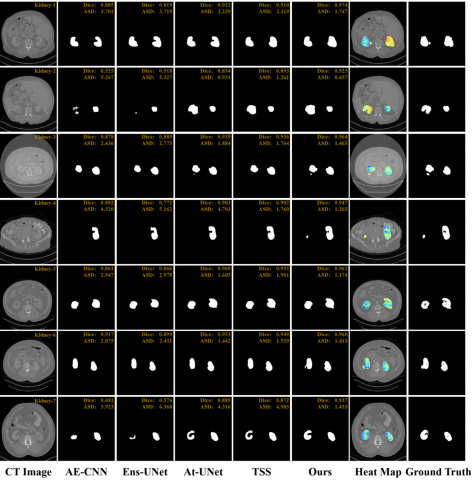
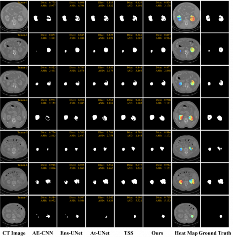
Figure 4. The qualitative segmentation outcomes for kidney segmentation
Qualitative Results: As shown in Figure 4, segmentation outcomes from AE-CNN [41], Ens-UNet [30], At-UNet [33], TSS [34], and our ERNet are compared across seven representative kidney cases. Heatmaps from ERNet are also visualized, where darker blue indicates greater pixel-level attention. Dice and ASD metrics are annotated in the top-right corner of each image to indicate segmentation accuracy. ERNet demonstrates superior performance, particularly in capturing edge details that are typically blurred and fused with the background. Kidney-3, 5, 6, and 7 highlight this advantage, closely matching the Ground Truth. At-UNet and TSS show partial improvements but fail to fully recover edge structures. Meanwhile, Kidney-1, 2, and 4 illustrate ERNet’s ability to recover regions with low heatmap weights, benefiting from the BP-trained bias model that refines pixel probabilities. Kidney-4, in particular, shows precise left kidney segmentation. Although visual results are compelling, ERNet’s quantitative performance also remains comparable to TSS and At-UNet.
2) Tumor Segmentation
Quantitative Results: Analyzing the tumor segmentation results in Table 1, it becomes evident that ERNet excels across most metrics. This advantage can be attributed to the common characteristic of tumors in the dataset, often presenting with blurred edges. Notably, ERNet is designed to address the issue of blurry edges prevalent in tumor segmentation. It achieves the best segmentation results with Dice=0.863 and Dice=0.855 for KiTS2019 and KiTS2021, respectively. These values bear testament to ERNet’s proficiency in achieving highly accurate segmentation. All methods exhibit negative RVD values, indicating that none of the methods’ predictions surpass the Ground Truth. In this context, a value closer to 0 signifies a prediction closer to the Ground Truth. ERNet similarly excels by achieving the nearest proximity to the Ground Truth in terms of the RVD metric among the methods.
Figure 5. Qualitative segmentation results for tumor segmentation
Qualitative Results: As shown in Figure 5, we compare tumor segmentation outcomes using AE-CNN, Ens-UNet, At-UNet, TSS, and our ERNet across seven representative cases. Heatmaps from ERNet highlight attention regions, where darker blue indicates greater pixel-level focus. Dice and ASD metrics are annotated in the upper-right of each case, with higher Dice and lower ASD values indicating more accurate segmentation. ERNet demonstrates a strong ability to capture intricate tumor edge details that are often missed by other methods. In Tumor-7, for instance, AE-CNN, Ens-UNet, and At-UNet provide minimal segmentation on the left side, while ERNet successfully avoids erroneous outputs in that area. This accuracy is attributed to the precise RoI constraints imposed by Mask R-CNN, which confine the segmentation to valid regions. Furthermore, the BP-trained bias model in ERNet only influences pixel probabilities within the defined RoI, enhancing its reliability in complex cases.
4.4 Ablation study
In this subsection, we conduct four experiments to verify the performance of each module of ERNet.
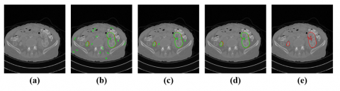
RoI. The RoI stands as a pivotal foundation within the framework of ERNet. This significance arises from ERNet’s bias model, which is learned during the training process and adapts to the entirety of the image. Throughout the training phase, we employ Eq. (2) to confine the heatmap within the bounds of the labeled region. This confinement facilitates the precise acquisition of the relationship between the Softmax pixel class probabilities, heatmap weights, and the Ground Truth.
Figure 6 presents a visual ablation of RoI settings. In (a), the original CT image is shown with the kidney in green and the tumor in red. Without any RoI constraints, as in (b), the globally applied heatmap during testing leads to minor false-positive segmentations due to ERNet’s reset probability. In (c), a coarse RoI—generated by enlarging the Mask R-CNN RoI by 0.5× in both length and width—still leads to potential misclassifications despite slightly lower overall error rates. Conversely, the precise RoI from Mask R-CNN in (d) effectively encloses the tumor, minimizing false segmentation results. In (e), the Ground Truth is displayed; the tumor is defined as part of the kidney, and the red overlay visually obscures the green region. This experiment underscores the importance of accurate RoI localization for suppressing spurious activations and enhancing segmentation reliability in ERNet.
Figure 6. RoI ablation experiment
Softmax. The core component of ERNet lies in its Softmax learning bias. In neural networks, when the features of target pixels within images fail to be prominently highlighted, it leading to the network’s tendency to misclassify these pixels during segmentation. The primary objective of Softmax learning bias is to lower the threshold at which these features, which are challenging to distinguish, are categorized as target pixels. To contrast the outcomes of not learning bias with ERNet’s learned bias, we compare the Mask RCNN for kidney tumor segmentation with ERNet in Table 2.
Table 2. Comparison of ERNet and mask RCNN for kidney and tumor segmentation
|
Method |
Blurry Edges |
Crisp Edges |
||
|
Kidney |
Tumor |
Kidney |
Tumor |
|
|
Mask RCNN [48] |
0.913 |
0.671 |
0.957 |
0.739 |
|
ERNet |
0.982 |
0.858 |
0.960 |
0.751 |
As observed from Table 2, ERNet excels in both kidney and tumor segmentation when compared to the basic Mask RCNN. This is attributed to ERNet’s capacity to identify those edge pixels with features that are not significantly pronounced, which are often overlooked by Mask RCNN. However, in scenarios where the target without blurry edges, ERNet’s performance closely aligns with that of Mask RCNN. Consequently, ERNet proves to be better suited for segmenting medical targets characterized by blurry edges.
Seg-Grad-CAM. ERNet’s objective revolves around reducing the classification threshold for poorly performing target pixels. During the training process, determining which pixels require resetting and learning becomes a critical consideration. The issue is expertly addressed through the interpretable heatmaps generated by Seg-Grad-CAM. This is due to the fact that pixels with lower contribution values tend to be positioned at the edge. Thus, by leveraging the heatmap weights derived from Seg-Grad-CAM, pixels can be categorized into distinct classes without necessitating additional clustering operations. As illustrated in Table 3, a comparison between unsupervised clustering based on grayscale values and bias learning through heatmap-guided segmentation underscores the effectiveness of the heat map approach. As the pixels within the RoI are progressively subdivided into multiple classes for bias learning, the Dice scores for kidney and tumor segmentation gradually improve. This demonstrates how the utilization of Seg-Grad-CAM’s heatmaps enables ERNet to distinguish between different pixel categories with greater precision, ultimately enhancing the segmentation results.
Table 3. Ablation experiments with Seg-Grad-CAM
|
|
Global Bias |
Kmeans-10 |
Kmeans-20 |
Kmeans-30 |
Heat Map (ERNet) |
|
Kidney |
0.485 |
0.684 |
0.753 |
0.871 |
0.964 |
|
Tumor |
0.173 |
0.385 |
0.592 |
0.738 |
0.863 |
BP. Fitting the pixel class probabilities and heatmap weights of Softmax using BP is the most straightforward and efficient approach. Despite various alternatives, such as Bayesian methods for bias fitting, BP has the advantage of leveraging its own neural units for more precise fitting. One notable advantage of BP in ERNet is its minimal requirement for additional parameter configuration, in contrast to other fitting methods that escalate the hyperparameter count. Furthermore, ERNet doesn’t necessitate interpretability or parameter explanations for the fitting process, rendering BP as a simpler choice for fitting.
4.5 Parameter settings
ERNet begins with an initial learning rate of 0.01 and a weight decay of 0.001. The images are sized at $512 \times 512$ , with a batch size of 4. RoI Align is set at a resolution of $7 \times 7$ , and the anchor's preset size is 64. The BP hidden layer consists of 5 neural units with a Sigmoid activation function. The update of weights is performed using stochastic gradient descent.
We proposed a novel edge-refining network called ERNet for the segmentation of kidney tumors in CT images. ERNet diverges from directly employing Softmax class probabilities for result determination; rather, it focuses on the precision segmentation of targets by resetting pixel class probabilities through interpretable heatmap weights. This approach particularly excels in accurately segmenting areas with blurry edges. Despite requiring more computational resources, ERNet showcases exceptional performance in segmenting medical images containing targets with ambiguous edges. ERNet’s effectiveness stems from its precise RoI limitation and interpretable heatmap, which facilitate the resetting of pixel class probabilities within the RoI while leaving the rest of the image unaffected. In the future, ERNet could be extended for segmenting other medical targets characterized by blurry edges.
This research was supported by the Science and Technology Project of Sichuan (Grant Nos. 2023ZHCG0008), and the Chengdu Science and Technology Project (Grant No: 2022-YF05-00068-SN).
[1] Liang, S., Gu, Y. (2023). SRENet: A spatiotemporal relationship-enhanced 2D-CNN-based framework for staging and segmentation of kidney cancer using CT images. Applied Intelligence, 53(13): 17061-17073. https://doi.org/10.1007/s10489-022-04384-5
[2] Liu, X., Zhao, Y., Wang, S., Wei, J. (2024). TransDiff: Medical image segmentation method based on Swin Transformer with diffusion probabilistic model. Applied Intelligence, 54(8): 6543-6557. https://doi.org/10.1007/s10489-024-05496-w
[3] Kaur, R., Juneja, M., Mandal, A.K. (2021). Machine learning based quantitative texture analysis of CT images for diagnosis of renal lesions. Biomedical Signal Processing and Control, 64: 102311. https://doi.org/10.1016/j.bspc.2020.102311
[4] Yang, A., Xu, L., Qin, N., Huang, D., Liu, Z., Shu, J. (2024). MFU-Net: A deep multimodal fusion network for breast cancer segmentation with dual-layer spectral detector CT. Applied Intelligence, 54(5): 3808-3824. https://doi.org/10.1007/s10489-023-05090-6
[5] Cao, G., Sun, Z., Wang, C., Geng, H., Fu, H., Sun, L., Nan, J. (2023). S2S-ARSNet: Sequence-to-Sequence automatic renal segmentation network. Biomedical Signal Processing and Control, 79: 104121. https://doi.org/10.1016/j.bspc.2022.104121
[6] Heiran, F., Khodaei-Mehr, J., Vatankhah, R., Sharifi, M. (2021). Nonlinear adaptive control of immune response of renal transplant recipients in the presence of uncertainties. Biomedical Signal Processing and Control, 63: 102163. https://doi.org/10.1016/j.bspc.2020.102163
[7] Alpar, O., Dolezal, R., Ryska, P., Krejcar, O. (2022). Low-contrast lesion segmentation in advanced MRI experiments by time-domain Ricker-type wavelets and fuzzy 2-means. Applied Intelligence, 52(13): 15237-15258. https://doi.org/10.1007/s10489-022-03184-1
[8] Si, T., Nayak, S., Sarkar, A. (2021). Kidney MRI segmentation for lesion detection using clustering with slime mould algorithm. In 2021 10th international conference on internet of everything, microwave engineering, communication and networks (IEMECON), Jaipur, India, pp. 1-6. https://doi.org/10.1109/IEMECON53809.2021.9689104
[9] Thomas, N.R., Anitha, J. (2022). An automated kidney tumour detection technique from computer tomography images. In 2022 International Conference on Computing, Communication, Security and Intelligent Systems (IC3SIS), Kochi, India, pp. 1-6. https://doi.org/10.1109/IC3SIS54991.2022.9885650
[10] Rao, Y., Lv, Q., Zeng, S., Yi, Y., Huang, C., Gao, Y., Sun, J. (2023). COVID-19 CT ground-glass opacity segmentation based on attention mechanism threshold. Biomedical Signal Processing and Control, 81: 104486. https://doi.org/10.1016/j.bspc.2022.104486
[11] Xuan, P., Cui, H., Zhang, H., Zhang, T., Wang, L., Nakaguchi, T., Duh, H.B. (2022). Dynamic graph convolutional autoencoder with node-attribute-wise attention for kidney and tumor segmentation from CT volumes. Knowledge-Based Systems, 236: 107360. https://doi.org/10.1016/j.knosys.2021.107360
[12] Hossain, M.S., Hassan, S.N., Al-Amin, M., Rahaman, M.N., Hossain, R., Hossain, M.I. (2023). Kidney disease detection from CT images using a customized CNN model and deep learning. In 2023 International Conference on Advances in Intelligent Computing and Applications (AICAPS), Kochi, India, pp. 1-6. https://doi.org/10.1109/AICAPS57044.2023.10074314
[13] Hussain, M.A., Hamarneh, G., Garbi, R. (2021). Cascaded regression neural nets for kidney localization and segmentation-free volume estimation. IEEE Transactions on Medical Imaging, 40(6): 1555-1567. https://doi.org/10.1109/TMI.2021.3060465
[14] Sadeghi, M.H., Zadeh, H.M., Behroozi, H., Royat, A. (2021). Accurate kidney tumor segmentation using weakly-supervised kidney volume segmentation in CT images. In 2021 28th National and 6th International Iranian Conference on Biomedical Engineering (ICBME), Tehran, Iran, pp. 38-43. https://doi.org/10.1109/ICBME54433.2021.9750362
[15] Qin, T., Wang, Z., He, K., Shi, Y., Gao, Y., Shen, D. (2020). Automatic data augmentation via deep reinforcement learning for effective kidney tumor segmentation. In ICASSP 2020-2020 IEEE International Conference on Acoustics, Speech and Signal Processing (ICASSP), Barcelona, Spain, pp. 1419-1423. https://doi.org/10.1109/ICASSP40776.2020.9053403
[16] Zhang, Y., Lu, D., Qiu, X., Li, F. (2023). Scattering-point-guided RPN for oriented ship detection in SAR images. Remote Sensing, 15(5): 1411. https://doi.org/10.3390/rs15051411
[17] Pandey, M., Gupta, A. (2022). An approach to remove extraneous slices from CT for kidney segmentation. In 2022 1st IEEE International Conference on Industrial Electronics: Developments & Applications (ICIDeA), Bhubaneswar, India, pp. 116-121. https://doi.org/10.1109/ICIDeA53933.2022.9970062
[18] Ranjbarzadeh, R., Dorosti, S., Ghoushchi, S.J., Caputo, A., Tirkolaee, E.B., Ali, S.S., Bendechache, M. (2023). Breast tumor localization and segmentation using machine learning techniques: Overview of datasets, findings, and methods. Computers in Biology and Medicine, 152: 106443. https://doi.org/10.1016/j.compbiomed.2022.106443
[19] Khalal, D.M., Azizi, H., Maalej, N. (2023). Automatic segmentation of kidneys in computed tomography images using U-Net. Cancer/Radiothérapie, 27(2): 109-114. https://doi.org/10.1016/j.canrad.2022.08.004
[20] Mehedi, M.H.K., Haque, E., Radin, S.Y., Rahman, M.A.U., Reza, M.T., Alam, M.G.R. (2022). Kidney tumor segmentation and classification using deep neural network on CT images. In 2022 International Conference on Digital Image Computing: Techniques and Applications (DICTA), Sydney, Australia, pp. 1-7. https://doi.org/10.1109/DICTA56598.2022.10034638
[21] Guo, J., Zeng, W., Yu, S., Xiao, J. (2021). RAU-Net: U-Net model based on residual and attention for kidney and kidney tumor segmentation. In 2021 IEEE international conference on consumer electronics and computer engineering (ICCECE), Guangzhou, China, pp. 353-356. https://doi.org/10.1109/ICCECE51280.2021.9342530
[22] Yan, X., Yuan, K., Zhao, W., Wang, S., Li, Z., Cui, S. (2020). An efficient hybrid model for kidney tumor segmentation in CT images. In 2020 IEEE 17th International Symposium on Biomedical Imaging (ISBI), Iowa City, IA, USA, pp. 333-336. https://doi.org/10.1109/ISBI45749.2020.9098325
[23] Sun, P., Mo, Z., Hu, F., Song, X., Mo, T., Yu, B., Chen, Z. (2022). Segmentation of kidney mass using AgDenseU-Net 2.5 D model. Computers in Biology and Medicine, 150: 106223. https://doi.org/10.1016/j.compbiomed.2022.106223
[24] da Cruz, L.B., Júnior, D.A.D., Diniz, J.O.B., Silva, A.C., de Almeida, J.D.S., de Paiva, A.C., Gattass, M. (2022). Kidney tumor segmentation from computed tomography images using DeepLabv3+ 2.5 D model. Expert Systems with Applications, 192: 116270. https://doi.org/10.1016/j.eswa.2021.116270
[25] Kang, L., Zhou, Z., Huang, J., Han, W. (2022). Renal tumors segmentation in abdomen CT Images using 3D-CNN and ConvLSTM. Biomedical Signal Processing and Control, 72: 103334. https://doi.org/10.1016/j.bspc.2021.103334
[26] Les, T., Markiewcz, T., Dziekiewicz, M., Lorent, M. (2021). Kidney segmentation from computed tomography images using U-Net and batch-based synthesis. In 2021 International Joint Conference on Neural Networks (IJCNN), Shenzhen, China, pp. 1-8. https://doi.org/10.1109/IJCNN52387.2021.9534007
[27] Tregidgo, H.F., Soskic, S., Althonayan, J., Maffei, C., et al. (2023). Accurate Bayesian segmentation of thalamic nuclei using diffusion MRI and an improved histological atlas. NeuroImage, 274: 120129. https://doi.org/10.1016/j.neuroimage.2023.120129
[28] Hertel, V., Chow, C., Wani, O., Wieland, M., Martinis, S. (2023). Probabilistic SAR-based water segmentation with adapted Bayesian convolutional neural network. Remote Sensing of Environment, 285: 113388. https://doi.org/10.1016/j.rse.2022.113388
[29] Vinogradova, K., Dibrov, A., Myers, G. (2020). Towards interpretable semantic segmentation via gradient-weighted class activation mapping (student abstract). In Proceedings of the AAAI conference on artificial intelligence, 34(10): 13943-13944. https://doi.org/10.1609/aaai.v34i10.7244
[30] Causey, J., Stubblefield, J., Qualls, J., Fowler, J., Cai, L., Walker, K., Huang, X. (2021). An ensemble of U-Net models for kidney tumor segmentation with CT images. IEEE/ACM Transactions on Computational Biology and Bioinformatics, 19(3): 1387-1392. https://doi.org/10.1109/TCBB.2021.3085608
[31] Ronneberger, O., Fischer, P., Brox, T. (2015). U-net: Convolutional networks for biomedical image segmentation. In International Conference on Medical Image Computing and Computer-Assisted Intervention, Munich, Germany, pp. 234-241. https://doi.org/10.1007/978-3-319-24574-4_28
[32] Hwang, G., Yoon, H., Ji, Y., Lee, S.J. (2022). RBCA-Net: Reverse boundary channel attention network for kidney tumor segmentation in CT images. In 2022 13th International Conference on Information and Communication Technology Convergence (ICTC), Jeju Island, Korea, pp. 2114-2117. https://doi.org/10.1109/ICTC55196.2022.9952992
[33] Geethanjali, T.M., Dinesh, M.S. (2021). Semantic segmentation of tumors in kidneys using attention U-Net models. In 2021 5th International Conference on Electrical, Electronics, Communication, Computer Technologies and Optimization Techniques (ICEECCOT), Mysuru, India, pp. 286-290. https://doi.org/10.1109/ICEECCOT52851.2021.9708025
[34] Hou, X., Xie, C., Li, F., Wang, J., Lv, C., Xie, G., Nan, Y. (2020). A triple-stage self-guided network for kidney tumor segmentation. In 2020 IEEE 17th International Symposium on Biomedical Imaging (ISBI), Iowa City, IA, USA, pp. 341-344. https://doi.org/10.1109/ISBI45749.2020.9098609
[35] Lu, J., Liu, R., Zhang, Y., Zhang, X., Zheng, L., Zhang, C., Lu, Y. (2022). Development and application of a detection platform for colorectal cancer tumor sprouting pathological characteristics based on artificial intelligence. Intelligent Medicine, 2(2): 82-87. https://doi.org/10.1016/j.imed.2021.08.003
[36] Li, S.T., Zhang, L., Guo, P., Pan, H.Y., Chen, P.Z., Xie, H.F., Wang, Y. (2023). Prostate cancer of magnetic resonance imaging automatic segmentation and detection of based on 3D-Mask RCNN. Journal of Radiation Research and Applied Sciences, 16(3): 100636. https://doi.org/10.1016/j.jrras.2023.100636
[37] Lu, J., Yao, J., Zhang, J., Zhu, X., Xu, H., Gao, W., Zhang, L. (2021). Soft: Softmax-free transformer with linear complexity. Advances in Neural Information Processing Systems, 34: 21297-21309.
[38] Stevens, J.R., Venkatesan, R., Dai, S., Khailany, B., Raghunathan, A. (2021). Softermax: Hardware/software co-design of an efficient Softmax for transformers. In 2021 58th ACM/IEEE Design Automation Conference (DAC), San Francisco, CA, USA, pp. 469-474. https://doi.org/10.1109/DAC18074.2021.9586134
[39] Gour, M., Jain, S. (2022). Automated COVID-19 detection from X-ray and CT images with stacked ensemble convolutional neural network. Biocybernetics and Biomedical Engineering, 42(1): 27-41. https://doi.org/10.1016/j.bbe.2021.12.001
[40] Valverde, J.M., Tohka, J. (2023). Region-wise loss for biomedical image segmentation. Pattern Recognition, 136: 109208. https://doi.org/10.1016/j.patcog.2022.109208
[41] Toğaçar, M., Muzoğlu, N., Ergen, B., Yarman, B.S.B., Halefoğlu, A.M. (2022). Detection of COVID-19 findings by the local interpretable model-agnostic explanations method of types-based activations extracted from CNNs. Biomedical Signal Processing and Control, 71: 103128. https://doi.org/10.1016/j.bspc.2021.103128
[42] Selvaraju, R.R., Cogswell, M., Das, A., Vedantam, R., Parikh, D., Batra, D. (2017). Grad-CAM: Visual explanations from deep networks via gradient-based localization. In Proceedings of the IEEE International Conference on Computer Vision, Venice, Italy, pp. 618-626. https://doi.org/10.1109/iccv.2017.74
[43] Wang, H., Wang, Z., Du, M., Yang, F., Zhang, Z., Ding, S., Hu, X. (2020). Score-CAM: Score-weighted visual explanations for convolutional neural networks. In Proceedings of the IEEE/CVF Conference on Computer Vision and Pattern Recognition Workshops, Seattle, WA, USA, pp. 24-25. https://doi.org/10.1109/cvprw50498.2020.00020
[44] Muhammad, M.B., Yeasin, M. (2020). Eigen-CAM: Class activation map using principal components. In 2020 International Joint Conference on Neural Networks (IJCNN), Glasgow, UK, pp. 1-7. https://doi.org/10.1109/IJCNN48605.2020.9206626
[45] He, K., Gkioxari, G., Dollár, P., Girshick, R. (2017). Mask R-CNN. In Proceedings of the IEEE International Conference on Computer Vision, pp. 2961-2969. https://doi.org/10.48550/arXiv.1703.06870
[46] Heller, N., Sathianathen, N., Kalapara, A., Walczak, E., Moore, K., Kaluzniak, H., Weight, C. (2019). The KiTS19 challenge data: 300 kidney tumor cases with clinical context, CT semantic segmentations, and surgical outcomes. arXiv preprint arXiv:1904.00445. https://doi.org/10.48550/arXiv.1904.00445
[47] University of Minnesota Robotics Institute (MnRI), Helmholtz Imaging Platform (HIP), Cleveland Clinic's Urologic Cancer Program. (2021). The 2021 Kidney and Kidney Tumor Segmentation Challenge. https://kits-challenge.org/kits21/.