Mohammad S. Khrisat* | Hatim Ghazi Zaini | Ziad A. Alqadi
© 2021 IIETA. This article is published by IIETA and is licensed under the CC BY 4.0 license (http://creativecommons.org/licenses/by/4.0/).
OPEN ACCESS
The process of digital image features extraction is very important and it is required in many applications such as classification, prediction and regression. The extracted features for each image must be unique and capable to be used as an image identifier. In this paper we will introduce a method of image features extraction; it will be shown that this method will enhance the efficiency of the features extraction process. The proposed method will be experimentally tested using various images; the obtained experimental results will be compared with other existing methods of feature extraction to show the advantages of the proposed method and to show how to increase the speed up of the method.
features vector, classification, speedup, throughput, k means clustering, WPT, composite vector
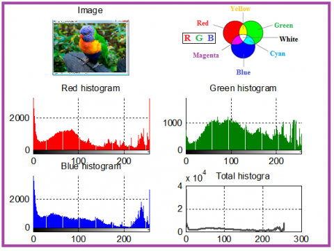
Digital color image is represented by a 2D matrix (gray image) [1, 2], or a 3D matrix (color image), each 2D matrix in the 3D matrix represents a color channel (red, green and blue). Digital gray image can be represented by a histogram [3, 4]. The histogram is a 1D array with 256 elements, each element points to the repetition of the pixel color in the image [5, 6]. Each color channel in color image also can be represented by histogram vector, adding the three vectors together we can get the color image total histogram (Total histogram=Red histogram array + green histogram array +blue histogram array) as shown in Figure 1.
Figure 1. Color image and the associated histograms
Image histogram can be used in many applications [7, 8], it can be used as an input data set for the image features extraction method, some of these methods are based on the image histogram such as wavelet packet tree (WPT) decomposition [9, 10].
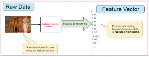
Digital images are used in many important applications such as image classification and recognition systems [11, 12]. Since the size of the image is very large, it is necessary to search for a way through which to extract a small number of values to represent the image and use these values as an identifier for the image (see Figure 2). The set of these values is called the vector of the features of the image [13, 14]. This vector must satisfy the following requirements [15, 16]:
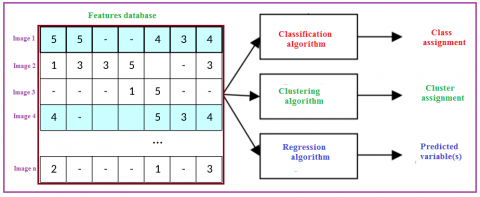
The extracted images features vectors must be stored in the features database, this database can be used as an input dataset for the classification or prediction tool (see Figure 3) in order to identify the image.
Clustering means grouping input data items(pixels values) into groups called clusters as shown in Figure 4 [17, 18]. One of the most popular methods of data clustering is kmeans clustering. This method can be used to cluster the input data into 2 or more clusters, the clusterin process can be used to retrieve valuable information, this information can be used to form the image features vector [19, 20].
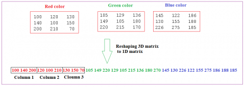
Kmeans clustering is a flexible method, it can be done by using 1D or 2D dimentional matrix as an input dataset, the digital colr image can be easily reshaped for 3D matrix to 1D array (see Figure 5), this array can be then clustered to find the following informations [21]:
One of the above mentioned information can be used to form the image features vector.
Figure 4. Data clustering
Figure 5. Reshaping example
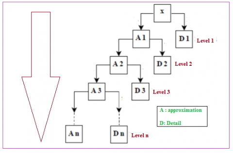
Wavelet packet tree (WPT) [22, 23] decomposition can be used to decompose a reshaped 3D color image matrix to 1D matrix to approximations and details based on using Haar equations [24]. The first level of decomposition split the input data into approximation and detail, the length of each of them is equal the half of the input data length (see Figure 6). Here the number of selected levels will determine the length of the features vector.
Figure 6. WPT decomposition
To extract the image features, we use the obtained approximation at the previous level as a new input data set for decomposition, by repeating this process for several determined levels we can obtain an approximation with the required number of elements to be used later as an image features vector.
Digital images have various sizes, so it is difficult to select the number of decomposition levels, so we can use the total color image histogram with 256 elements to get the image features using WPT decomposition [25].
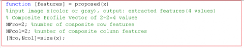
The proposed method of image features extraction can be implemented applying the following steps:
Step 1: Get the image, and retrieve the image size (rows and columns: Nro, Ncol).
Step 2: Determine the features vector length, here we have to select the number of composite rows and columns (NFro and NFcol), and the features vector length will equal NFro + NFcol.
Step 3: Calculate the average of each row in the image to from comRo vector.
Step 4: Calculate the average of each column in the image to from comCol vector.
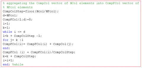
Step 5: Aggregate the comRo vector of Nro elements into compFro vector of NFro elements.
Step 6: Aggregate the comCol vector of Ncol elements into compFcol vector of NFcol elements.
Step 7: Composite features vector of compFro and compFcol.
Below is a matlab function that can be used to implement the proposed method:
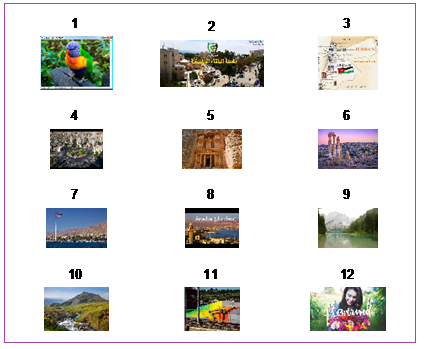
Several images (see Figure 7) with various sizes were selected, the features vector length with length = 4 was selected, Table 1 show the obtained experimental results:
Figure 7. Used images
From Table 1 we can see the following:
The proposed method is flexible; it can be easily changed to create a feature vector with any length by adjusting NFro and NFcol parameters, Table 2 shows the features vector with length =6 for the same selected images, here the average extraction time remain small.
The same images were treated using kmeans clustering, 4 clusters were selected, and the clusters centroids were selected as a features vector, Table 3 shows the obtained experimental results.
Table 1. Proposed method results (features vector length=4)
|
Image number |
Resolution |
Size(byte) |
Features |
Extraction time (seconds) |
|||
|
1 |
151 333 3 |
150849 |
150.1636 |
90.0209 |
125.1993 |
114.8626 |
0.034000 |
|
2 |
152 171 3 |
77976 |
214.2279 |
212.2096 |
218.8906 |
207.5312 |
0.015000 |
|
3 |
360 480 3 |
518400 |
110.0616 |
62.6860 |
86.1564 |
86.5912 |
0.040000 |
|
4 |
1071 1600 3 |
5140800 |
99.1678 |
103.8407 |
122.4715 |
80.5573 |
0.243000 |
|
5 |
981 1470 3 |
4326210 |
164.6155 |
90.8392 |
126.3232 |
129.0533 |
0.170000 |
|
6 |
165 247 3 |
122265 |
118.0844 |
91.4567 |
88.7047 |
120.1296 |
0.020000 |
|
7 |
360 480 3 |
518400 |
100.7605 |
64.4090 |
88.8745 |
76.2950 |
0.039000 |
|
8 |
183 275 3 |
150975 |
150.5115 |
104.4943 |
140.8969 |
114.5462 |
0.022000 |
|
9 |
183 275 3 |
150975 |
139.5991 |
81.9698 |
118.3683 |
102.8616 |
0.021000 |
|
10 |
201 251 3 |
151353 |
74.5080 |
100.4746 |
98.7142 |
76.6994 |
0.019000 |
|
11 |
600 1050 3 |
1890000 |
158.0257 |
115.0430 |
148.9100 |
124.1587 |
0.105000 |
|
12 |
1144 1783 3 |
6119256 |
133.0626 |
139.3956 |
146.5038 |
125.9705 |
0.252000 |
|
Average |
1.6098e+006 |
Throughput=1.6098e+006/0.0817=1.9704e+007 byte per second |
0.0817 |
||||
Table 2. Proposed method results (features vector length=6)
|
Image number |
Features |
Extraction time (seconds) |
|||||
|
1 |
186.4707 |
78.6212 |
95.1849 |
126.7492 |
122.2955 |
110.9450 |
0.023000 |
|
2 |
212.9356 |
208.8769 |
217.2241 |
225.4204 |
216.1531 |
198.0828 |
0.017000 |
|
3 |
109.5097 |
102.1804 |
47.4313 |
90.7175 |
87.7056 |
80.6983 |
0.043000 |
|
4 |
94.3544 |
109.3746 |
100.8142 |
143.7382 |
98.2167 |
62.5882 |
0.174000 |
|
5 |
192.2893 |
103.6399 |
87.1356 |
132.5569 |
110.3678 |
140.1400 |
0.153000 |
|
6 |
111.6450 |
131.4171 |
70.2296 |
81.5154 |
100.6012 |
131.1751 |
0.020000 |
|
7 |
94.6460 |
101.2674 |
51.8409 |
94.3294 |
81.1034 |
72.3215 |
0.045000 |
|
8 |
177.4976 |
85.3655 |
119.9428 |
130.9332 |
137.9840 |
113.8887 |
0.020000 |
|
9 |
157.4983 |
92.3999 |
81.8265 |
115.7081 |
116.3203 |
99.6964 |
0.021000 |
|
10 |
59.3113 |
109.3241 |
94.5084 |
103.6602 |
95.4630 |
64.0205 |
0.020000 |
|
11 |
172.6813 |
137.1078 |
99.8140 |
141.4802 |
142.5161 |
125.6068 |
0.089000 |
|
12 |
135.4069 |
127.1200 |
145.9410 |
149.1750 |
138.6913 |
120.8210 |
0.196000 |
|
Average |
0.0684 |
||||||
Table 3. Kmeans clustering method results (features vector length=4)
|
Image number |
Features |
Extraction time (seconds) |
|||
|
1 |
231.4323 |
25.5328 |
90.8931 |
165.3871 |
1.203000 |
|
2 |
150.1751 |
238.7813 |
57.9272 |
205.8391 |
0.604000 |
|
3 |
11.1279 |
122.7569 |
189.0679 |
64.5786 |
3.404000 |
|
4 |
132.1343 |
27.7147 |
197.7589 |
79.0318 |
19.121000 |
|
5 |
51.3912 |
161.2255 |
224.6232 |
100.6020 |
26.189000 |
|
6 |
122.5739 |
169.7968 |
33.0259 |
83.5358 |
0.815000 |
|
7 |
6.2029 |
225.4998 |
140.4629 |
81.2838 |
3.414000 |
|
8 |
152.3228 |
35.1126 |
235.1358 |
92.7938 |
0.898000 |
|
9 |
137.3452 |
33.2478 |
202.4468 |
85.7968 |
0.512000 |
|
10 |
80.2431 |
19.3801 |
151.1589 |
218.0935 |
1.773000 |
|
11 |
111.8570 |
55.6583 |
237.6980 |
177.7467 |
9.501000 |
|
12 |
228.0653 |
109.4986 |
61.9170 |
147.7168 |
25.402000 |
|
|
Throughput=1.6098e+006/ 7.7363=2.0808e+005 byte per second |
7.7363 |
|||
Table 4. WPT method results (features vector length=4)
|
Image number |
Features |
Extraction time (seconds) |
|||
|
1 |
28382 |
26681 |
5214 |
9242 |
0.119000 |
|
2 |
1290 |
1147 |
-643 |
11567 |
0.117000 |
|
3 |
312000 |
281610 |
29680 |
6940 |
0.122000 |
|
4 |
577200 |
535750 |
325920 |
94500 |
0.128000 |
|
5 |
57800 |
53390 |
241240 |
158630 |
0.127000 |
|
6 |
11343 |
10058 |
8725 |
1535 |
0.150000 |
|
7 |
715770 |
639140 |
25430 |
13710 |
0.119000 |
|
8 |
1962 |
2411 |
5707 |
15281 |
0.142000 |
|
9 |
12669 |
11671 |
9351 |
3003 |
0.115000 |
|
10 |
51161 |
47444 |
7019 |
4406 |
0.153000 |
|
11 |
-2900 |
5910 |
59860 |
227090 |
0.176000 |
|
12 |
8940 |
-50560 |
430150 |
156530 |
0.124000 |
|
|
Throughput=1.6098e+006/ 0.1327=1.2131e+007 byte per second |
0.1327 |
|||
Table 5. Proposed method speedup
|
Method |
Average extraction time(seconds) |
Speedup |
||
|
Proposed |
WPT |
Kmeans |
||
|
Proposed |
0.0817 |
1 |
0.1327/0.0817=1.6242 |
7.7363/0.0817=94.6916 |
|
WPT |
0.1327 |
0.0817/ 0.1327=0.6157 |
1 |
7.7363/0.1327=58.2992 |
|
Kmeans |
7.7363 |
0.0817/7.7363=0.0106 |
0.1327/7.7363=0.0172 |
1 |
From Table 3 we can see the following:
The same images were treated using WPT method, the image histogram was taken as an input dataset for decomposition, and Table 3 shows the obtained experimental results.
From Table 4 we can see the following:
From the previous obtained results we can see that the proposed method will speed up the process of image features extraction process, this is shown in Table 5.
A method of digital image features extraction was proposed and implemented. The proposed method can be used for any type of images and with any sizes. The proposed method is very efficient simple and accurate. Comparisons with other methods of features extraction were done based on the obtained experimental results. The results showed that the propose method has a speed up greater than 1, this means that this method will increase the extraction process efficiency. It was shown that the proposed method is very flexible, miner a simple change can be done to obtain a features vector with any length, the extracted image features satisfies the requirements of image features to be used as a classifier.
[1] Shivaprasad, S., Sadanandam, M. (2021). Optimized features extraction from spectral and temporal features for identifying the Telugu dialects by using GMM and HMM. Ingénierie des Systèmes d’Information, 26(3): 275-283. https://doi.org/10.18280/isi.260304
[2] Chu, W., Hung, W.C., Tsai, Y.H., Chang, Y.T., Li, Y.J., Cai, D., Yang, M.H. (2021). Learning to caricature via semantic shape transform. International Journal of Computer Vision, 129: 2663-2679. https://doi.org/10.1007/s11263-021-01489-1
[3] Zou, D.N., Zhang, S.H., Mu, T.J., Zhang, M. (2020). A new dataset of dog breed images and a benchmark for finegrained classification. Computational Visual Media, 6: 477-487. https://doi.org/10.1007/s41095-020-0184-6
[4] le Négrate, A., Beghdadi, A., Dupoisot, H. (1992). An image enhancement technique and its evaluation through bimodality analysis. CVGIP: Graphical Models and Image Processing, 54(1): 13-22. https://doi.org/10.1016/1049-9652(92)90030-2
[5] Ackar, H., Almisreb, A.A., Saleh, M.A. (2019). A review on image enhancement techniques. Southeast Europe Journal of Soft Computing, 8(1): 42-48. http://dx.doi.org/10.21533/scjournal.v8i1.175
[6] Lin, H.Y., Lin, C.Y., Lin, C.J., Yang, S.C., Yu, C.Y. (2014). A study of digital image enlargement and enhancement. Mathematical Problems in Engineering, 2014: 1-7. https://doi.org/10.1155/2014/825169
[7] Cromey, D.W. (2012). Digital images are data: And should be treated as such. In: Taatjes D., Roth J. (eds) Cell Imaging Techniques. Methods in Molecular Biology (Methods and Protocols), vol 931. Humana Press, Totowa, NJ. https://doi.org/10.1007/978-1-62703-056-4_1
[8] Gitto, S., Cuocolo, R., Emili, I., Tofanelli, L., Chianca, V., Albano, D., Messina, C., Imbriaco, M., Sconfienza, L.M. (2021). Effects of interobserver variability on 2D and 3D CT- and MRI-based texture feature reproducibility of cartilaginous bone tumors. Journal of Digital Imaging, 34: 820-832. https://doi.org/10.1007/s10278-021-00498-3
[9] Benton, J.F., Gillespie, A.R., Soha, J.M. (1979). Digital image-processing applied to the photography of manuscripts. In: Scriptorium, 33(1): 40-55. https://doi.org/10.3406/scrip.1979.1119
[10] Wiggins, W.F., Caton, M.T., Magudia, K., Rosenthal, M.N., Andriole, K.P. (2021). A conference-friendly, hands-on introduction to deep learning for radiology trainees. Journal of Digital Imaging, 34: 1026-1033. https://doi.org/10.1007/s10278-021-00492-9
[11] El-Khamy, S.E., Hadhoud, M.M., Dessouky, M.I., Salam, B.M., Abd El-Samie, F.E. (2014). An iterative method for the evaluation of the regularization parameter in regularized image restoration. International Journal of Computing, 8(2): 15-23. https://doi.org/10.47839/ijc.8.2.662
[12] Korsunov, N.I., Toropchin, D.A. (2016). The method of finding the spam images based on the hash of the key points of the image. International Journal of Computing, 15(4): 259-264. https://doi.org/10.47839/ijc.15.4.857
[13] Yu, T., Meng, J., Fang, C., Jin, H., Yuan, J. (2020). Product quantization network for fast visual search. International Journal of Computer Vision, 128: 2325-2343. https://doi.org/10.1007/s11263-020-01326-x
[14] Ansari, M.D., Ghrera, S.P. (2016). Feature extraction method for digital images based on intuitionistic fuzzy local binary pattern. 2016 International Conference System Modeling & Advancement in Research Trends (SMART), pp. 345-349. https://doi.org/10.1109/SYSMART.2016.7894547
[15] Wang, Z., Yong, J. (2008). Texture analysis and classification with linear regression model based on wavelet transform. IEEE Transactions on Image Processing, 17(8): 1421-1430. https://doi.org/10.1109/TIP.2008.926150
[16] Chen, C.C., Chen, C.C. (1999). Filtering methods for texture discrimination. Pattern Recognition Letters, 20(8): 783-790. https://doi.org/10.1016/S0167-8655(99)00042-2
[17] Chang, T., Jay Kuo, C.C. (1992). Tree-structured wavelet transform for textured image segmentation. Proc. SPIE 1770, Advanced Signal Processing Algorithms, Architectures, and Implementations III. https://doi.org/10.1117/12.130945
[18] Çarkacıoǧlu, A., Yarman-Vural, F. (2003). SASI: A generic texture descriptor for image retrieval. Pattern Recognition, 36(11): 2615-2633. https://doi.org/10.1016/S0031-3203(03)00171-7
[19] Tang, C., Yang, X., Zhai, G. (2015). Noise estimation of natural images via statistical analysis and noise injection. IEEE Transactions on Circuits and Systems for Video Technology, 25(8): 1283-1294. https://doi.org/10.1109/TCSVT.2014.2380196
[20] Nader, J., Alqadi, Z.A., Zahran, B. (2017). Analysis of color image filtering methods. International Journal of Computer Applications, 174(8): 12-17. https://doi.org/10.5120/ijca2017915449
[21] Unser, M. (1986). Local linear transforms for texture measurements. Signal Processing, 11(1): 61-79. https://doi.org/10.1016/0165-1684(86)90095-2
[22] Walia, S., Kumar, K. (2019). Digital image forgery detection: A systematic scrutiny. Australian Journal of Forensic Sciences, 51(5): 488-526. https://doi.org/10.1080/00450618.2018.1424241
[23] Al Azzeh, J., Alhatamleh, H., Alqadi, Z.A., Abuzalata, M.K. (2016). Creating a color map to be used to convert a gray image to color image. International Journal of Computer Applications, 153(2): 31-34. https://doi.org/10.5120/ijca2016911975
[24] Khawatreh, S., Ayyoub, B., Abu-Ein, A., Alqadi, Z. (2018). A novel methodology to extract voice signal features. International Journal of Computer Applications, 179(9): 40-43. https://doi.org/10.5120/ijca2018916088
[25] Ayyoub, B., Nader, J., Al-Qadi, Z., Zahran, B. (2019). Suggested method to create color image features victor. Journal of Engineering and Applied Sciences, 14(1): 2203-2207. https://doi.org/10.36478/jeasci.2019.2203.2207