OPEN ACCESS
The performance of automatic control systems hinges on the parameters of proportional–integral–derivative (PID) controller. Therefore, this paper attempts to determine the most suitable parameter values of PID controller. For this purpose, the particle swarm optimization (PSO) was improved after introducing the flying time T and adaptive weight ω, and the improved PSO (IPSO) was compared against the basic PSO and the PSO modified with both inertial weight and constriction factor (PSO-ω, x). After that, the IPSO was applied to optimize the parameters of the PID controller. With a second-order inertia model as the control object, the parameters of PID controller optimized by the IPSO were contrasted with those optimized by the traditional Ziegler–Nichols optimization method. The results show that the IPSO is faster and more accurate than the traditional approach. The research findings provide new insights into the optimization of the PID controller and the application of the PSO.
flying time, adaptive weight, constriction factor, improved particle swarm optimization (ipso), proportional–integral–derivative (PID) controller
The proportional–integral–derivative (PID) controller is a robust and simple control loop feedback mechanism, which has been widely applied for the digital PID control in the manufacturing of electronics, machines, chemicals and metal products. The control effect depends on the proportional gain constant kp, the integral gain ki and the derivative gain kd, while the control error hinges on the proportional, integral and derivative terms (denoted as P, I and D, respectively) of the object (Yu and Yan, 2006). However, it is very difficult to find the most suitable parameters of the PID controller. To overcome the difficulty, many new methods have been developed to determine the parameters that ensure the stable auto-optimization and adaptive control of the PID controller (Sun et al., 2004).
Traditionally, the parameters of PID controller are optimized numerically or graphically using trail-and-error against Bode plots. Recent years has seen the proliferation of intelligent optimization algorithms in parameter optimization of PID controller, including but not limited to genetic algorithm (GA), ant colony algorithm (ACA), seeker optimization algorithm (SOA) and particle swarm optimization (PSO) (Yu et al., 2013; Tao et al., 2012). Among them, the PSO, proposed by Kennedy and Eberhart (1998), has been extensively applied to optimize the parameters of the PID controller at home and abroad. On the upside, the PSO enjoys a simple structure, high accuracy, fast convergence and strong adaptability. Particularly, the algorithm can be extended for multi-objective optimization. On the downside, the PSO faces slow convergence and undesirable accuracy in certain conditions (Atyabi and Samadzadegan, 2011; Meng et al., 2013).
Considering the above, this paper introduces the flying time T and adaptive weight ω to the PSO algorithm, and compares the improved PSO (IPSO) against the basic PSO and the PSO modified with both inertial weight and constriction factor (PSO-ω, x). The experimental results verify that the IPSO can achieve high accuracy and fast convergence. Next, the IPSO was applied to optimize the parameters of the PID controller (Ono and Nakayama, 2009). The control object is a second-order inertia model. The IPSO-based optimization outperformed the traditional parameter optimization method for PID controller (Ziegler–Nichols optimization method) (Gong et al., 2011; Yang et al., 2010; Yu and Cao, 2014).
The PSO was first intended for simulating social behaviors of bird flocks or fish schools. This algorithm has been widely adopted for parameter optimization in high-dimensional spaces, thanks to its simple structure, search efficiency and fast global convergence.
2.1. The basic PSO
The basic PSO works by having a population (called swarm) of z candidate solutions (called particles), which are interested in approximating the global minimum x0 of the objective function f: Rn→R. These particles are moved around in the search-space D according to a few simple formulae. The movements of the particles are guided by their own best known position Xz(pbest) in the search-space as well as the entire swarm’s best known position Xgbest. The position of particle z is determined by the solution of the objective function. In each iteration, the position is updated and represented by a vector Xlz∈Rn.
The position of particle z is updated based on its current velocity Vlz ∈Rn and the previous position Xl-1z:
${{X}_{l}}^{z}={{X}_{l-1}}^{z}+{{V}_{l}}^{z}$ (1)
The vector Vl-1z is updated by the formula below:
${{V}_{l}}^{z}~={{V}_{l-1}}^{z}~+{{c}_{1}}\Xi ({{X}^{z\left( pbest \right)}}-{{X}_{l-1}}^{z})+{{c}_{2}}\Xi ({{X}^{gbest}}-{{X}_{l-1}}^{z})$ (2)
where Vl-1z is the previous velocity of particle z; Ξ is a diagonal matrix of random numbers in the interval [0, 1]; c1 is the cognitive parameter reflecting the effect of individual experience on the decision-making of the next particle; c2 is the social parameter reflecting the effect of social experience on the decision-making of the next particle. Together, the two parameters characterize the trend of velocity update. The previous studies have recommended the following values for c1 and c2: c1=c2=2, c1=c2=2.05 or c1>c2 with c1+c2<=4.10.
Figure 1. Particle movement
It can be seen from Figure 1 and Equation (2) that the particle velocity is updated in three phases. The flow chart of the basic PSO is presented in Figure 2 below.
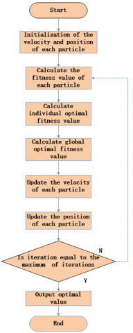
Figure 2. Flow chart of the basic PSO
It can be seen that the basic PSO contains the three key steps below:
(1) Initialize the swarm size z.
(2) Randomly select an Xlz from the interval [Xmax, Xmin] that obeys uniform distribution.
(3) Randomly select a Vlz from the interval [Vmax, Vmin] that obeys uniform distribution.
2.2. Variants
Some variants of the PSO have been developed to enhance its velocity, stability or convergence. A well-known variant is called the PSO with inertial weight (PSO-ω), which either fixes or reduces the inertial weight. The basic idea is to balance the local and global searches with the addition of the inertial weight ω. The impact of ω on the velocity update of each particle can be expressed as:
$V_{l}^{z}=\omega V_{l-1}^{z}+c_{1} \Xi\left(X^{z(p b e s t)}-X_{l-1}^{z}\right)+c_{2} \Xi\left(X^{g b e s t}-X_{l-1}^{z}\right)$ (3)
The value of the inertial weight ω is positively correlated with the global search ability of the algorithm and negatively with the local search ability. In other words, a large inertial weight helps to avoid the local minimum trap and boost the global search, while a small inertial weight facilitates the accurate local search and promotes the convergence of the algorithm.
Many different PSO variants can be created according to different weight update formulas, such as linear weight decreasing PSO, adaptive weight PSO and random weight PSO. For example, the linear weight decreasing PSO can prevent the premature convergence and oscillation against the global optimum of the basic PSO.
Currently, the most accepted strategy of inertial weight is to establish ω∈ [ωmin; ωmax] and reduce its value according the number of the current iteration:
$\omega=\omega=\omega_{m a x}-\frac{\left(\omega_{m a x}-\omega_{m m}\right)}{I t r_{m a x}} l$ (4)
where Itrmax is the maximum number of iterations. The recommended values are ωmax=0.9 and ωmin=0.4.
The basic PSO can be viewed as a special case in which the inertial weight is set to 1 throughout the iterations.
For better control of particle velocity, the constriction factor x can be introduced:
$V_{l}^{z}=\chi\left[V_{l-1}^{z} \omega+c_{1} \Xi\left(X^{z(p b e s t)}-X_{l-1}^{z}\right)+c_{2} \Xi\left(X^{g b e s t}-X_{l-1}^{z}\right)\right]$ (5)
Where
$x=\frac{2}{|2-\varphi-\sqrt{\varphi^{2}-4 \varphi}|}$ (6)
and φ=c1+c2>4.
The recommended value of x is 0.729 with c1=c2=2. The PSO modified with both inertial weight and constriction factor is denoted as the PSO-ω, x.
2.3. The IPSO
The basic PSO was improved with the addition of flying time T and adaptive weight ω, aiming to enhance the stability and convergence speed. The adaptive weight ω can be updated as:
$\omega(l)=C \cdot e^{(F(l) / F(l-1))}$ (7)
where ω(l) is the adaptive weight of the l-th iteration; F(l) is the global best fitness of the l-th iteration; C is the compressibility factor, which is a constant. The impact of ω(l) on the velocity update of each particle can be expressed as:
$V_{l}^{z}=\omega(l) \bullet V_{l-1}^{z}+c_{1} \Xi\left(X^{z(p b s t)}-X_{l-1}^{z}\right)+c_{2} \Xi\left(X^{g b s t}-X_{l-1}^{z}\right)$ (8)
The flying time T is updated according to the following expression
$T=t \bullet\left(1-\frac{k \bullet l}{l t r_{m x x}}\right)$ (9)
where t is the initial flying time; k is an adjusting factor, which is a constant. The impact of T on the positive update of each particle can be expressed as:
$X_{l}^{z}=X_{l-1}^{z}+T \bullet V_{l}^{z}$ (10)
The IPSO can be implemented in the following steps:
(1) Initialize the swarm size, particle positions and particle velocities
(2) Calculate the fitness of each particle.
(3) Compare the fitness of each particle with its own best known fitness, and make it the new best known fitness if it is better than the latter.
(4) Compare the fitness of each particle with the global best known fitness, and make it the new global best known fitness if it is better than the latter.
(5) Update the velocity and position of each particle according to Equations (8) and (10).
(6) Output the solution if the termination condition is satisfied; Otherwise, return to Step (2).
2.4. Verification of the IPSO with classical functions
Five classical functions (Table 1) were selected to compared the IPSO with the basic PSO and the PSO-ω, x. The pseudocodes of the basic PSO, the PSO-ω, x and the IPSO are given in Tables 2~4, respectively. The parameters settings of the three PSOs are listed in Table 5. During the verification, the solution of the classical functions was restricted in the range shown in Table 6. The results of the three PSOs relative to the five classical functions are recorded in Table 7. Figures 3~7 compare the results of all three PSOs obtained through 200 iterations.
Table 1. The selected classical function
|
Classical Function |
|
$f_{1}(x)=\sum_{i=1}^{10} x_{i}^{2}$ |
|
$f_{2}\left(x_{1}, x_{2}\right)=20+x_{1}^{2}+x_{2}^{2}-10 \cdot\left[\cos \left(2 \pi \cdot x_{1}\right)+\cos \left(2 \pi \cdot x_{2}\right)\right]$ |
|
$f_{3}(x, y)=0.5+\frac{\sin ^{2} \sqrt{x^{2}+y^{2}}-0.5}{\left[1+0.001\left(x^{2}+y^{2}\right)^{2}\right]^{2}}$ |
|
$f_{4}(x)=418.929 n+\sum_{i=1}^{n} x_{i} \sin \left(\left|x_{i}\right|^{1 / 2}\right)$ |
|
$f_{s}\left(x_{1}, x_{2}\right)=100\left(\mathrm{x}_{1}^{2}-x_{2}^{2}\right)+\left(1-\mathrm{x}_{1}^{2}\right)$ |
Table 2. Pseudo-code for basic PSO algorithm
|
Data: c1c2ZItrmaxωmaxωmin |
|
|
Generete randomly X0z and V0z for Z particles of the swarm; Evaluate F(X0z) for each particle,; The minimum valueof F(X0z) for each particle is Fmin; update Xz(best)and Xgbest; for l=1 to l=ltrmaxdo for z=1 to z=Z do Update Vlz with Eq.(3); Update Xlz with Eq.(1); Compute F(Xlz), seethe classical function; Update Fmin; Update Xz(pbest); End |
|
|
End |
|
|
Update Xgbest; Verify stopping criteria;SolutionXgbest; |
|
Table 3. Pseudo-code for PSO with ω and x algorithm
|
Data: c1c2ZItrmaxx ω |
|
|
Generete randomly X0z and V0z for Z particles of the swarm; Evaluate F(X0z) for each particle,; The minimum valueof F(X0z) for each particle is Fmin; update Xz(best)and Xgbest; for l=1 to l=ltrmaxdo for z=1 to z=Z do Update Vlz with Eq.(5); Update Xlz with Eq.(1); Compute F(Xlz), seethe classical function; UpdateFmin; Update Xz(pbest); End |
|
|
End |
|
|
Update Xgbest; Verify stopping criteria; Solution Xgbest; |
|
Table 4. Pseudo-code for improved PSO algorithm
|
Data: c1c2ZItrmaxt k |
|
|
Generete randomly X0z and V0z for Z particles of the swarm; Evaluate F(X0z) for each particle,; The minimum valueof F(X0z) for each particle is Fmin; update Xz(best)and Xgbest; for l=1 to l=ltrmaxdo for z=1 to z=Z do Update Vlz with Eq.(8); Update Xlz with Eq.(10); Compute F(Xlz),seethe classical function; UpdateFmin; Update Xz(pbest); End |
|
|
End |
|
|
Update Xgbest; Verify stopping criteria;SolutionXgbest; |
|
Table 5. The parameter settings ofthree PSOs
|
Basic PSO |
PSO withω and x |
Improved PSO |
|
c1=1.49, c2=1.49 Z=50, Itrmax=200 ωmax =0.91, ωmin = 0.45 |
c1=1.49, c2=1.49 Z=50, Itrmax=200 χ=0.729, ω=1 |
c1=1.49, c2=1.49 Z=50, Itrmax=200 T=0.6, k=0.9 |
Table 6. The range of values of the classical function
|
The classical function |
The range of values |
|
$f_{1}(x)$ |
|x|<=15 |
|
$f_{2}\left(x_{1}, x_{2}\right)$ |
x1,x2∈[-5,5] |
|
$f_{3}(x, y)$ |
x,y∈[-10,10] |
|
$f_{4}(x)$ |
x∈[-500,500] |
Table 7. The optimization values obtained by the three PSO methods
|
Classical function |
Target value |
Basic PSO |
PSO withω and x |
Improved PSO |
|
$f_{1}(x)$ |
0 |
1.65 e-04 |
8.70 e-05 |
2.00 e-09 |
|
$f_{2}\left(x_{1}, x_{2}\right)$ |
0 |
4.73 e-04 |
2.86 e-05 |
3.79 e-06 |
|
$f_{3}(x, y)$ |
0 |
2.73 e-08 |
1.47 e-10 |
1.30 e-11 |
|
$f_{4}(x)$ |
0 |
1.31 e-04 |
2.67 e-04 |
2.50 e-08 |
|
$f_{5}\left(x_{1}, x_{2}\right)$ |
0 |
1.47e-05 |
2.73e-05 |
3.67 e-08 |
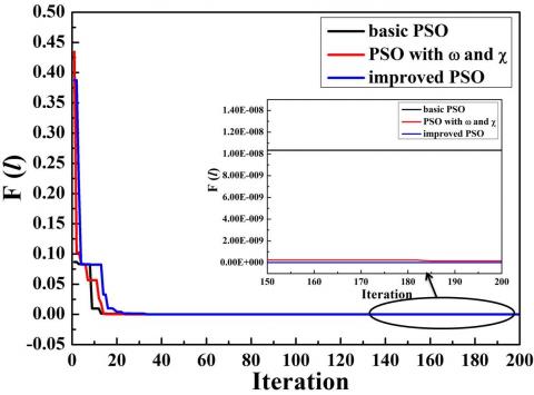
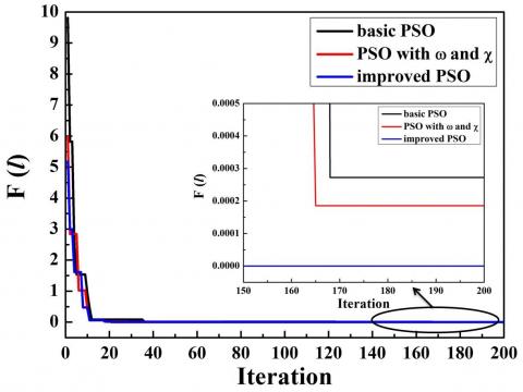
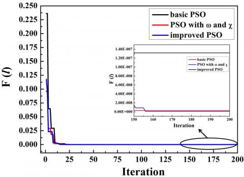
As shown in Table 7, the IPSO outputted 2.00 e-09 for f1(x), 3.79 e-06 for f2(x1, x2), 1.30 e-11 for f3(x, y), 1.30 e-11 for f4(x) and 3.67 e-08 for f5(x1, x2), while the target values of f1(x)~ f5(x1, x2) are all zero. Compared to the contrastive algorithms, the IPSO approximated the theoretical value. According to Figures 5~9, the IPSO achieved the fastest convergence while the basic PSO the slowest convergence. Suffice it to say that the IPSO can greatly enhance the solution quality.
Figure 3. F(l) value obtained by f1(x) for each iteration of the three PSO methods
Figure 4. F(l) value obtained by f2(x1, x2) for each iteration of the three PSO methods
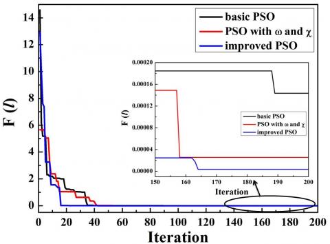
Figure 5. F(l) value obtained by f3(x,y) for each iteration of the three PSO methods
Figure 6. F(l) value obtained by f4(x) for each iteration of the three PSO methods
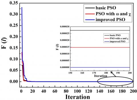
Figure 7. F(l) value obtained by f5(x) for each iteration of the three PSO methods
3.1. Parameter optimization problem of PID controller
In an industrial control system, the output of a control object exhibits as an S-shaped rising curve under the action of a step signal. In this case, the output can be described by a second-order inertia transfer function:
$G(S)=\frac{K}{T_{1} \bullet S^{2}+T_{2} \bullet S+T_{3}}$ (11)
The PID controller is the most popular regulator tool in engineering. Since its birth 70 years ago, the PID controller has become the main technology of industrial control due to its simplicity, stability, reliability and flexibility. It is particularly suitable for objects that cannot be understood clearly with common theories. Based on system error, the PID control technology computes the control value based on the proportional, integral and derivative terms of the object. The control parameters of PID controller are detailed as follows.
(1) Proportional
The error signal is proportional to the scale of control system. Upon detection of an error, the controller will perform an action to control the error. The response speed and adjustment accuracy are positively correlated with the value of the proportional gain constant kp. However, it is easy to produce overshoot, which leads to shock and instability in a certain range.
(2) Integral
The integral action aims to eliminate the static error, thus enhancing the stability and response speed of the system. The effect of the integral action is negatively correlated with the integral time constant Ts. The greater the constant is, the weaker the integral action, and the faster the elimination of the static error. Nevertheless, the integral action is likely to cause saturation in the initial phase, and worsen the overshoot in the response phase.
(3) Differential
The differential parameter reveals the variation in the error signal. To speed up system operation and shorten the adjustment time, the differential time constant TD is introduced before the change takes place to the error signal. The differential action reduces the error in response to any direction and predicts the error in advance. Nonetheless, this action may force the response to stop early and lengthen the adjustment time.
The parameters of PID controller should remain constant in the reproduction process. Any variation in TD, Ts and KP will harm the control effect of the PID controller.
Suppose the error e and control action u satisfy the following equation:
$u(t)=K_{p}\left[e(t)+\frac{1}{T_{s}} \int_{0}^{t} e(t) \quad d t+T_{D} \frac{e(t)-e(t-1)}{d t}\right]$ (12)
where e(t) is the error function; u(t) is the t function of the control action; dt is the sampling period; TD is the differential time constant; Ts is the integral time constant; KP is the proportional gain constant.
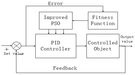
Figure 8. Schematic diagram of traditional PID
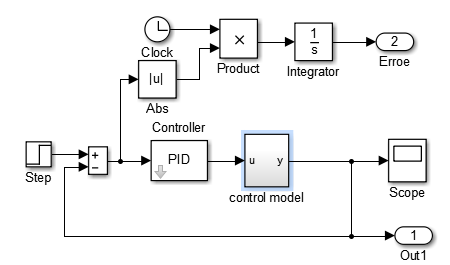
The traditional PID contoller is shown in Figure 8, where rin(t) is the set value and yout(t) is the output value. The goal of parameter optimization is to find the proper KP, Tsand TD of the PID controller, such that the solution of the fitness function F=∫0∞|e(t)|tdt is minimized. The fitness function is illustrated in Figure 9, where Step is the set point.
The parameter optimization of PID controller is a complex nonlinear programming problem. So far, there has not been a mathematical formula that can accurately express the relationship between parameters of PID controller and the objective function. To make up for the gap, the IPSO was applied to solve the problem. As shown in Figure 9, the error of the control system is the difference between the set value and the response. The Abs refers to the absolute value of the error; the Error is the integration between the clock and the absolute error.
Figure 9. PID simulation mode
3.2. Tuning results
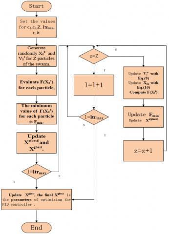
The IPSO-based parameter optimization of PID controller is explained in Figures 10 and 11. The goal is to obtain the best parameters that ensure the optimal PID control effect.
Figure 10. Flow chart of Optimizing PID parameters with the improved PSO
Figure 11. Schematic diagram of Optimizing PID parameters with the improved PSO
The optimization inputs include the following data: the parameters of the object (T1=7.69e-3, T2=2.3e-5, T3=291 and K=3508), the parameters of the IPSO (c1=1.49, c2=1.49, Z=50, Itrmax=200, T=0.6 and k=0.9). The control object is a second-order inertial model:
$G(S)=\frac{3508}{7.69 \cdot 10^{-3} S^{2}+2.3 \cdot 10^{-5} S+291}$ (13)
The PID control output ya constant is unit step response. To verify the effect of IPSO-based optimization, the control effect of the IPSO-optimized parameters was contrasted with that of the parameters optimized by the traditional parameter optimization method for PID controller (Ziegler–Nichols optimization method).
Table 8. The Ziegler-Nichols tuning method
|
Ziegler–Nichols method |
|||
|
Control Type |
Kp |
TS |
TD. |
|
P |
0.5 Ku |
- |
- |
|
PI |
0.45Ku |
Tu/1.2 |
- |
|
PD |
0.8Ku |
- |
Tu/8 |
|
Classic PID |
0.6 Ku |
Tu/2 |
Tu/8 |
|
Peesen Inter Rule |
0.7 Ku |
Tu/2.5 |
3Tu/20 |
|
Some overshoot |
0.33 Ku |
Tu/2 |
Tu/3 |
|
No overshoot |
0.2 Ku |
Tu/2 |
Tu/3 |
The Ziegler–Nichols optimization method is a heuristic method developed by John G. Ziegler and Nathaniel B. Nichols. It is performed by setting the I (integral) and D (derivative) gains to zero. The P (proportion) gain Kp is then increased (from zero) until it reaches the ultimate gain Ku, at which the output of the control loop has stable and consistent oscillations. The Ku and the oscillation period Tu are used to set the P, I and D gains depending on the controller used.
Table 9. Pseudo-code for Optimization of PID parameters with improved PSO algorithm
|
Data: c1c2ZItrmaxtk |
|
|
Generete randomly X0z and V0z for Z particles of the swarm; Evaluate F(X0z) for each particle, $F=\int_{0}^{\infty}|e(t)| \mathrm{t} d t$; The minimum valueof F(X0z) for each particle is Fmin; update Xz(best)and Xgbest; for l=1 to l=ltrmaxdo for z=1 to z=Z do Update Vlz with Eq.(8); Update Xlz with Eq.(10); Compute F(Xlz),seethe classical function; UpdateFmin; Update Xz(pbest); End |
|
|
End |
|
|
Update Xgbest; Verify stopping criteria;SolutionXgbest, Xgbest isresults of optimization parameters |
|
Table 10. Parameters obtained by the three PSO methods and Z-N
|
Parameter |
Improved PSO |
Z-N |
|
KP |
2.9 |
3.6 |
|
TS |
1.8212 |
2.3076 |
|
TD. |
0.01978 |
0.05616 |
|
Time |
0.1509 s |
0.2599 s |
The results of the comparison test are displayed in Table 10 and Figure 12. It can be seen from the table that the IPSO reached the equilibrium faster than the traditional method. Figure 12 shows a small overshoot and fast convergence to the set value, indicating that the IPSO-based optimization outperformed the traditional method.
Figure 12. Response of PID control system
In order to optimize the control effect of the PID controller, this paper improves the PSO by replacing the fixed weight with the adaptive weight and introducing the flying time. Then, the IPSO was validated through comparison with the basic PSO and the PSO-ω, x. After that, the IPSO was applied to optimize the parameters of the PID controller. With a second-order inertia model as the control object, the IPSO-optimized parameters of PID controller were contrasted with those optimized by the traditional parameter optimization method for PID controller (Ziegler–Nichols optimization method). The comparison shows that the IPSO outperformed the traditional method in both convergence speed and accuracy. The research findings shed new light on the parameter optimization of the PID controller and the application of the PSO.
Atyabi A., Samadzadegan S. (2011). Particle swarm optimization-a survey. Applications of Swarm Intelligence, pp. 167-179.
Gong D. W., Zhang J. H., Zhang Y. (2011). Multi-objective particle swarm optimization for robot path planning in environment with danger sources. Journal of Computers, Vol. 6, No. 8, pp. 1554-1561. http://dx.doi.org/10.4304/jcp.6.8.1554-1561
Kennedy J. (1998). The behavior of particles. Evolutionary Programming VII, pp. 581-590. http://dx.doi.org/10.1007/BFb0040809
Meng L., Han P., Ren Y., Wang D. (2013). Design of PID controller based on multi-objective particle swarm optimization algorithm. Computer Simulation, Vol. 30, No. 7, pp. 388-391.
Ono S., Nakayama S. (2009). Multi-objective particle swarm optimization for robust optimization and its hybridization with gradient search. IEEE International Conference on Evolutionary Computations, pp. 1629-1636. http://dx.doi.org/10.1109/CEC.2009.4983137
Sun J., Feng B., Xu W. B. (2004). A global search strategy of quantum behaved particle swarm optimization. IEEE Conf. on Cybernetics and Intelligent Systems Piscataway, pp. 111-116. http://dx.doi.org/10.1109/ICCIS.2004.1460396
Tao X. M., Liu F. R., Liu Y., Tong Z. J. (2012). Multi-scale cooperative mutation particle swarm optimization algorithm. Journal of Software, Vol. 23, No. 7, 1805-1815. http://dx.doi.org/10.1007/s10957-016-0959-1
Yang Z., Chen Z., Fan Z., Li X. (2010). Tuning of PID controller based on improved paticle-swarm-optimization. Control Theory & Application, Vol. 27, No. 10, 1345-1352.
Yu G., Liu G., Liu Z. F., Liu X. (2013). Multi-objective optimal planning of distributed generation based on quantum differential evolution algorithm. Power System Protection and Control, No. 14, 66-72.
Yu S., Cao Z. (2014). Optimization parameters of PID controller parameters based on seeker optimization algorithm. Computer Simulation, Vol. 31, No. 9, 347-350.
Yu T. M., Yan D. S. (2006). Differential evolution algorithm formulti-objective optimization. Journal of Changchun University of Technology, Vol. 16, No. 4, pp. 77-80.