Jian Han*![]() | Ye Liu
| Ye Liu![]() | Chaozheng Li
| Chaozheng Li![]()
© 2025 The authors. This article is published by IIETA and is licensed under the CC BY 4.0 license (http://creativecommons.org/licenses/by/4.0/).
OPEN ACCESS
Head and neck squamous cell carcinoma (HNSCC) remains a malignancy with a persistently high recurrence rate, substantially compromising long-term survival outcomes. Conventional risk stratification methods, which are primarily dependent on static clinical indicators, often fail to capture dynamic post-treatment variations and consequently provide limited predictive precision. To address this limitation, a static–dynamic dual-branch feature fusion model was developed for recurrence prediction following radiotherapy in HNSCC. The model comprises two complementary feature extraction pathways: a static branch employing fully connected neural networks to encode single-timepoint clinical attributes, and a dynamic branch using long short-term memory (LSTM) networks to characterize longitudinal clinical trajectories before and after treatment. A gated attention mechanism was incorporated to achieve adaptive weighting and fusion of branch outputs, and a classification head was used to estimate recurrence risk. The framework was trained and evaluated on a rigorously curated cohort of 147 patients with HNSCC, with performance assessed through five-fold cross-validation. Results demonstrated consistent improvements over conventional machine learning (ML) approaches and single-branch models across both three-year and five-year recurrence prediction tasks, yielding maximal accuracy of 0.944 and an area under the receiver operating characteristic curve (AUC) of 0.943. Notably, the proposed approach exhibited superior discriminative power in low false-positive ranges, underscoring its clinical applicability in high-stakes decision-making contexts. These findings establish the value of integrating complementary static and dynamic clinical information within a unified deep learning (DL) framework, offering a methodological advance for precise recurrence risk prediction in HNSCC. Beyond prognostic accuracy, this strategy provides a potential tool for personalized follow-up planning and more refined clinical risk stratification, thereby contributing to the optimization of survivorship care in patients with head and neck malignancies.
head and neck squamous cell carcinoma (HNSCC), recurrence prediction, deep learning (DL), dual-branch feature fusion, time-series modeling
HNSCC is an important component of the global cancer burden. Epidemiological data show that the annual incidence and mortality of HNSCC are considerable, ranking it among the most common malignant tumours worldwide [1, 2]. The disease involves multiple anatomical subsites such as the oral cavity, pharynx, and larynx, and presents significant clinical and biological heterogeneity; even after radical comprehensive treatment, recurrence and distant metastasis remain the core challenges limiting long-term survival [3]. In the United States, for example, approximately 53,000 new cases and 10,800 deaths from HNSCC occur each year; even with standardized treatment, about 25-50% of patients experience local persistence/recurrence (P/R) within 3 years after treatment, highlighting the urgent clinical need to identify high-risk individuals for recurrence after radiotherapy (or comprehensive treatment) at an early stage in order to optimize follow-up frequency and individualized intensification/de-intensification strategies [4-6].
Traditional recurrence/survival risk assessment mainly relies on clinicopathological indicators, such as Tumor–Node–Metastasis (TNM) stage, tumour volume, Human Papillomavirus (HPV) status, etc., but these static indicators are limited in characterizing minimal residual disease after treatment and the dynamic response of tumours to therapy, and thus cannot provide strong discriminative power for individualized risk stratification [7, 8]. Therefore, radiomics and ML have been widely explored: in multicentre populations, high-dimensional features of texture, shape, and intensity extracted from PET and CT fusion can improve risk assessment ability for different endpoints [9, 10]; at the same time, CT-radiomics has also shown potential in predicting HPV status and local control [11]. However, traditional radiomics is sensitive to feature engineering and preprocessing workflows, and cross-centre consistency and generalization still need to be continuously improved; although deep learning (DL) in medical imaging has developed rapidly, it still faces methodological challenges in terms of data scale, annotation quality, and external reusability [12, 13].
In recent years, DL and multimodal fusion strategies have promoted significant progress in HNSCC prognosis/recurrence prediction. A Cochrane systematic review in 2025 summarized the evidence of prediction models for radiotherapy-related complications of head and neck tumours (NTCP models), and explicitly emphasized the critical importance of external validation, study design quality, and methodological rigour for model usability [14]; meanwhile, the continuous evolution of modern radiotherapy techniques and the introduction of artificial intelligence have provided a technical basis for safer and more effective treatment and follow-up management [15]. In the specific scenario of “post-radiotherapy recurrence”, radiomics/deep models based on early PET/CT and clinical information after radiotherapy have shown early discrimination potential for local persistence/recurrence [4, 16]. Furthermore, from the perspective of multimodal and multilevel fusion, on the one hand, multicentre studies have shown that multilevel (image/matrix/feature) fusion of PET+CT can robustly improve prognostic prediction performance [10]; on the other hand, multicentre cohort studies combining clinical, CT-radiomics, and dosiomics/dosimetric information have also verified the generalizability and robustness of fusion strategies in real-world multi-domain data. In summary, existing evidence supports the organic integration of “static single-timepoint information” and “pre–post (or multi-timepoint) dynamic changes” within the same framework to achieve stable discrimination of individual recurrence risk that is closer to clinical workflows [12, 13, 17, 18].
Based on the above background and methodological inspiration, this study proposes a Static-Dynamic Dual-branch Feature Fusion Model (SDDFF-Model) for recurrence prediction after radiotherapy in HNSCC: one branch is used to represent key static features at a single timepoint, and the other branch is used to capture longitudinal variation features before and after treatment (such as contrast differences and temporal trajectories of images before and after radiotherapy); and an adaptive weight allocation strategy is used to integrate the outputs of the two branches to achieve information complementarity, aiming at long-term risk assessment of “recurrence after radiotherapy”.
The main contributions of this study include:
(1) A static feature modelling method based on fully connected neural networks is proposed, which effectively captures pathological and treatment-related features of patients at specific timepoints before and after radiotherapy, forming high-level semantic static representations and providing a stable feature basis for recurrence risk prediction.
(2) A longitudinal clinical data sequence at key timepoints before and after radiotherapy is constructed, and the temporal dependency is modelled using LSTM networks, which can fully characterize the dynamic evolution of body composition and nutritional status during treatment, thereby enhancing the sensitivity of the model to recurrence trends.
(3) A static–dynamic dual-branch fusion framework is designed, in which a gated attention mechanism adaptively allocates weights to static and dynamic features, achieving dynamic weighted fusion at the feature level and improving the expressive ability and predictive robustness of the model in complex clinical scenarios.
(4) On a real clinical dataset of HNSCC, three-year and five-year recurrence prediction experiments were carried out, respectively. The results show that the proposed method achieved better performance than comparison methods under different prediction windows, verifying the effectiveness and generalization potential of the model.
2.1 Overall architecture design
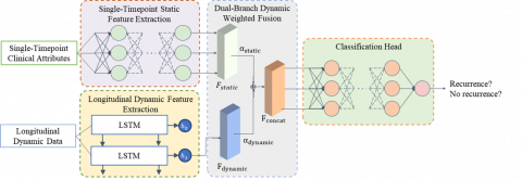
To address the technical challenges of multimodal time-series feature modelling in recurrence prediction of HNSCC after radiotherapy, an SDDFF-Model is proposed. As shown in Figure 1, the model adopts a differentiated feature processing strategy, scientifically dividing clinically collected data into two dimensions: static features at a single timepoint and dynamic features of longitudinal changes. In static feature modelling, the framework employs a fully connected neural network to conduct deep representation learning of single-timepoint features, precisely characterizing the physiological and pathological state of the patient at a specific time. In dynamic feature modelling, an LSTM network is used to perform time-series modelling of pre–post comparison features, effectively capturing the dynamic evolution patterns and temporal dependencies of longitudinal features during follow-up before and after radiotherapy. To fully utilize the complementary advantages of static and dynamic information, the framework designs a dual-branch dynamic weighted feature fusion mechanism, which integrates the outputs of the two branches through an adaptive weight allocation strategy, constructing a more comprehensive and expressive integrated feature representation. Finally, the fused feature vector is input into the classification head to achieve precise prediction and quantitative assessment of recurrence risk after radiotherapy in patients.
Figure 1. Overall architecture of the SDDFF-Model for recurrence prediction of HNSCC after radiotherapy
2.2 Single-timepoint static feature extraction strategy
The static feature branch takes as input the single-timepoint clinical attributes recorded during patient follow-up before and after radiotherapy, denoted as $x_{\text {static }} \in \mathbb{R}^{d_s}$, where $d_s$ is the dimension of static features. These features usually include demographic characteristics, tumour pathological characteristics, and treatment-related parameters, which can reflect the overall pathological and treatment status of patients at a specific time point.
This branch employs a multilayer fully connected neural network for deep representation learning of static information. The calculation process is as follows:
$z_1=W_1 x_{\text {static }}+b_1$, (1)
$\hat{z}_1=B N\left(z_1\right)$, (2)
$a_1=\sigma\left(\hat{z}_1\right)$, (3)
where, $W_1 \in \mathbb{R}^{d_h \times d_s}$ and $b_1 \in \mathbb{R}^{d_h}$ are the weight matrix and bias vector of the first layer, respectively, $B N(\cdot)$ denotes batch normalisation, and $\sigma(\cdot)$ is the activation function (such as ReLU). For a multilayer fully connected network, the above process can be recursively represented as:
$z_l=W_1 a_{l-1}+b_l$, (4)
$\hat{z}_l=B N\left(z_l\right)$, (5)
$a_l=\sigma\left(\hat{z}_l\right)$, (6)
After nonlinear transformations through L fully connected layers, the final feature representation of the static branch is:
$F_{\text {static }}=a_L \in \mathbb{R}^{d_f}$ (7)
where, $d_f$ is the dimension of the final feature representation, and $F_{\text {static}}$ contains high-level semantic features of the patient's static status.
2.3 Longitudinal dynamic feature extraction strategy
The dynamic feature extraction branch processes the feature vectors of patients at two key timepoints: pre-radiotherapy features $\mathrm{x}_1^{\text {dynamic }} \in \mathbb{R}^{\mathrm{d}_{\mathrm{d}}}$ and post-radiotherapy features $x_2^{\text {dynamic }} \in R^{d_d}$, where $d_d$ denotes the dimension of dynamic features. These two timepoint features are constructed into a time series: $X_{\text {dynamic }}=\left[x_1^{\text {dynamic }}, x_2^{\text {dynamic }}\right] \in \mathbb{R}^{2 \times d_d}$.
The LSTM network models this time series, and its forward propagation process can be expressed as follows:
For time step $t\in\{1,2\}$:
$f_t=\sigma\left(W_f \cdot\left[h_{t-1}, x_t^{\text {dynamic}}\right]+b_f\right)$, (8)
$i_t=\sigma\left(W_i \cdot\left[h_{t-1}, x_t^{\text {dynamic}}\right]+b_i\right)$, (9)
$\widetilde{C}_t=\tanh \left(W_C \cdot\left[h_{t-1}, x_t^{\text {dynamic}}\right]+b_C\right)$, (10)
$C_t=f_t \odot C_{t-1}+i_t \odot \widetilde{C}_t$, (11)
$o_t=\sigma\left(W_o \cdot\left[h_{t-1}, x_t^{\text {dynamic }}\right]+b_o\right)$, (12)
$h_t=o_t \odot \tanh \left(C_t\right)$. (13)
where, $f_t, i_t$, and $o_t$ are the forget gate, input gate, and output gate, respectively; $C_t$ is the cell state; $h_t$ is the hidden state; $W_*$ and $b_*$ are the corresponding weight matrices and bias vectors; and $\odot$ denotes element-wise multiplication.
The final feature representation of the dynamic branch is the hidden state at the last time step.
$F_{\text {dynamic}}=h_2 \in R^{d_f}$ (14)
2.4 Dual-branch feature dynamic weighted fusion mechanism
The dual-branch feature dynamic weighted fusion mechanism adaptively fuses the static feature $F_{\text {static}}$ and the dynamic feature $F_{\text {dynamic}}$. First, feature alignment ensures that the output dimensions of the two branches are consistent, and then a gated attention mechanism is used to calculate dynamic weights.
The concatenated representation of the fused features is expressed as:
$F_{\text {concat }}=\left[F_{\text {static }} ; F_{\text {dynamic }}\right] \in \mathbb{R}^{2 \times d_f}$, (15)
The attention weights of each branch are calculated through a gated network:
$\alpha_{\text {static}}=\sigma\left(W_s F_{\text {concat}}+b_s\right)$ (16)
$\alpha_{\text {dynamic }}=\sigma\left(W_d F_{\text {concat }}+b_d\right)$ (17)
where, $W_s, W_d \in \mathbb{R}^{1 \times 2 d_f}, b_s, b_d \in \mathbb{R}$ are learnable parameters, enabling the model to adaptively lear the optimal combination strategy of static and dynamic information in different patient groups.
The final fused feature representation is:
$F_{\text {fused }}=\alpha_{\text {static}} \cdot F_{\text {static}}+\alpha_{\text {dvnamic}} \cdot F_{\text {dvnamic}}$ (18)
This fused feature integrates the patient's baseline clinical state and treatment response dynamics, providing a more comprehensive information basis for recurrence risk assessment, where $\alpha_{\text {static }}+ \alpha_{\text {dynamic }}=1$. The fused feature $F_{\text {fused }}$ is input into the classification head (fully connected network) to perform the final recurrence probability prediction:
$y_{\text {pred}}=\operatorname{softmax}\left(W_{\text {cls}} F_{\text {fused }}+b_{\text {cls}}\right)$ (19)
where, $y_{\text {pred }} \in \mathbb{R}^C$ is the predicted probability distribution. C is the number of classes in the classification task. For the binary classification recurrence prediction task, C=2 (recurrence/non-recurrence).
The model adopts the cross-entropy loss function for end-to-end training to minimize the difference between the predicted probability and the true recurrence label:
$\mathcal{L}=-\frac{1}{N} \sum_{i=1}^N \sum_{j=1}^C y_{\text {true }}^{(i, j)} \log \left(y_{\text {pred }}^{(i, j)}\right)$ (20)
where, N is the batch size, and $y_{\text {true }}^{(i, j)}$ is the one-hot encoding of the true label. Gradient descent is used to optimize the network parameters to improve the accuracy of recurrence prediction.
3.1 Dataset
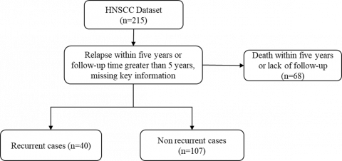
This study conducted all experiments and comparative analyses based on the publicly available dataset of HNSCC from MD Anderson Cancer Center. This dataset originates from 2,840 consecutively admitted HNSCC patients receiving radical radiotherapy between 2003 and 2013, and after screening, contains 215 patients who simultaneously had whole-body PET-CT scans or abdominal CT scans before and after radiotherapy. Since the original imaging data has ceased to be publicly accessible, this study used the corresponding Head-Neck-CT-Atlas Clinical Data clinical information for analysis. This clinical dataset provides complete patient information, including demographic characteristics, risk factors, tumor pathological features (grading, staging, site), treatment plan, recurrence status, and survival data [19].
According to the dataset construction criteria shown in Figure 2 (using five-year recurrence prediction as an example), 215 patients were further screened: 68 patients who died within five years or lacked sufficient follow-up data were excluded, and finally, 147 patients with clinical data meeting the research requirements were obtained. This dataset was divided into two groups according to the five-year recurrence status: 40 recurrence cases (27.2%) and 107 non-recurrence cases (72.8%), constituting the specialized clinical dataset for recurrence prediction after radiotherapy.
This study adopted a 5-fold cross-validation strategy to partition the data of 147 patients: patients were stratified and randomly grouped according to recurrence status to ensure that the proportion of recurrence and non-recurrence patients was consistent in each fold. Specifically, each fold contained about 29–30 patients, including 8 recurrence cases and 21–22 non-recurrence cases. In each validation, 4-folds (about 118 patients) were selected as the training set, and the remaining 1-fold (about 29 patients) was used as the test set. Five rounds of validation were performed to ensure that all patient data were used for model evaluation.
Figure 2. Dataset construction flowchart (taking five-year recurrence prediction as an example)
3.2 Data preprocessing
The data collected in this study are divided into single-time point static data and longitudinal change data before and after treatment. Appendix I displays static indicators, while Appendix II includes dynamic indicators before and after radiotherapy.
Data preprocessing is a key step in constructing the dual-branch deep learning model. First, the collected clinical data of 147 patients were subjected to quality assessment and missing value processing, with multiple imputation used to fill in missing data, and samples with data completeness lower than 80% were excluded. Then the features were divided into two categories for differential processing according to their temporal attributes: static features include patient basic information (sex, age, height), disease characteristics (diagnosis, TNM stage, pathological grade), treatment plan (chemotherapy plan, radiotherapy parameters), and lifestyle factors, etc. Continuous variables were standardized using Z-score, and categorical variables were encoded using one-hot encoding, label encoding, or binary encoding according to their nature, to ensure that the fully connected network could effectively learn the static state features of patients.
Dynamic change features mainly include body weight, BMI, L3-level muscle cross-sectional area, fat cross-sectional area, and their derived muscle index and fat index before and after treatment. These features constitute pre-post comparison time series data, which, after standardization, were input into the LSTM network to capture the dynamic evolution patterns of patient nutritional status and body composition during radiotherapy. Through this hierarchical preprocessing strategy, static features were fully represented, and dynamic features effectively reflected the treatment-related time-dependent changes, laying the data foundation for subsequent feature fusion and recurrence prediction.
3.3 Experimental environment and training settings
The experimental environment was configured as follows: CPU: Intel Core i7-14900KF @ 3.20GHz; operating system: Ubuntu 22.04 LTS; GPU: NVIDIA GeForce RTX 4060, CUDA version 11.7; Python version 3.10; deep learning framework: PyTorch 2.0.1.
For the training of the dual-branch deep learning recurrence prediction model, considering the small dataset scale (147 patients), the following training strategy was employed: the Adam optimizer was used to optimize network parameters, with weight decay set to 1e-4 to prevent overfitting and an initial learning rate set to 0.001. Due to the adoption of 5-fold cross-validation and limited sample size, the batch size was set to 16 to ensure sufficient samples per batch for gradient estimation. The model was trained for 200 epochs with a cosine annealing learning rate schedule (CosineAnnealingLR), and the minimum learning rate was set to 1e-6 to achieve smoother convergence. An early stopping mechanism was introduced, stopping training automatically when validation performance did not improve for 20 consecutive epochs, preventing overfitting and improving training efficiency. To enhance model generalization, dropout (p=0.3) was applied to the static feature branch, and recurrent dropout (p=0.2) was applied to the LSTM branch during training.
3.4 Evaluation metrics
Five widely used metrics were employed to quantitatively evaluate the classification results of five-year recurrence prediction:
Accuracy: measures the proportion of correctly predicted samples, defined as:
Accuracy $=\frac{T P+T N}{T P+T N+F P+F N}$
where, TP is true positives, TN is true negatives, FP is false positives, and FN is false negatives.
Precision: evaluates the proportion of true positive samples among predicted positive samples, defined as:
Precision $=\frac{T P}{T P+F P}$
Recall: measures the proportion of true positive samples identified among all true positive samples, defined as:
Recall $=\frac{T P}{T P+F N}$
F1-Score: harmonic mean of precision and recall, comprehensively evaluating model performance, defined as:
$F 1-$ Score $=2 \times \frac{\text {Precision} \times \text {Recall}}{\text {Precision}+ \text {Recall}}$
The F1-Score ranges from 0 to 1, with higher values indicating better balance between precision and recall.
Area Under the Receiver Operating Characteristic Curve (AUC): evaluates overall classifier performance at different thresholds, defined as the area under the ROC curve:
$A U C=\int_0^1 T P R(t) d F P R(t)$
where, TPR is the true positive rate and FPR is the false positive rate. AUC ranges from 0 to 1, with values closer to 1 indicating stronger discriminative ability and 0.5 indicating a random guessing level.
3.5 Horizontal comparison
To objectively evaluate the comprehensive advantages of the proposed dual-branch fusion model, this study conducted comparisons with five methods. All methods were evaluated under the same stratified 5-fold cross-validation, using unified feature standardization, missing value processing, and class weighting strategies. Evaluation metrics included Accuracy, Precision, Recall, and F1. Horizontal comparison results for three-year and five-year recurrence prediction tasks are reported, along with confusion matrix and ROC curve analyses.
3.5.1 Three-year recurrence experiment
The 5-fold cross-validation results in Table 1 indicate that the proposed SDDFF model exhibits excellent performance in the three-year recurrence prediction task. This model significantly outperforms traditional machine learning baseline methods in key metrics, including Accuracy, Precision, Recall, and F1, achieving 0.944±0.038, 0.857±0.117, 0.857±0.132, and 0.857±0.099, respectively. Compared with the best-performing traditional method, Random Forest, the SDDFF model achieved improvements of 5.5 and 14.3 percentage points in Accuracy and F1, respectively. Compared with Support Vector Machine (SVM), Gradient Boosting, Logistic Regression, and Multi-layer Perceptron (MLP), the proposed model achieved the highest Precision and tied for the best Recall with SVM, validating the effectiveness of multi-feature fusion and deep learning architecture in recurrence prediction. Moreover, the relatively small standard deviation across metrics indicates strong model stability, generalization ability, and robustness. Regression path analysis further confirms model reliability, providing a solid foundation for clinical decision support system deployment.
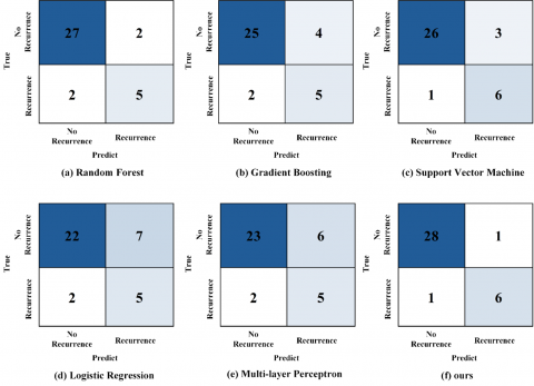
The confusion matrix analysis of comparison methods for the three-year follow-up window is shown in Figure 3. In the test set containing 36 samples, 7 were negative and 29 were positive. The proposed SDDFF model demonstrates excellent classification performance, with 28 true negatives, 1 false positive, 1 false negative, and 6 true positives, corresponding to high Accuracy, Precision, Recall, and F1 values of 0.944, 0.857, 0.857, and 0.857, respectively. Comparative analysis with traditional baselines shows F1 values of 0.750 for SVM, 0.714 for Random Forest, 0.625 for Gradient Boosting, 0.556 for MLP, and 0.526 for Logistic Regression. Notably, the SDDFF model excels in controlling false positives, producing only 1 misclassification, while SVM also maintains a low false negative count of 1. This feature achieves a better balance between Precision and Recall. Overall statistical and variance analysis indicate that the proposed method significantly outperforms traditional machine learning algorithms in classification accuracy and stability, providing more reliable technical support for recurrence risk prediction.
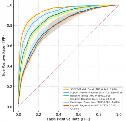
Figure 4 shows the ROC curve performance comparison of the comparison methods for the three-year follow-up recurrence prediction task. The average ROC curve of the proposed SDDFF model forms an upper envelope over most false positive rate intervals, with an AUC value of 0.943±0.010, significantly superior to SVM (0.918±0.012), Random Forest (0.880±0.015), Gradient Boosting (0.867±0.019), MLP (0.805±0.029), and Logistic Regression (0.797±0.026). The gray error band represents the standard deviation range across fold mean points, indicating that the proposed method maintains stable separation across the full curve and low cross-fold fluctuation compared with baseline algorithms, demonstrating better robustness and generalization ability. The SDDFF model not only achieves the optimal performance in the area under the curve metric, but its small standard deviation further confirms the consistency and reliability of model prediction performance, providing more precise discriminative ability for clinical recurrence risk assessment.
Table 1. Three-year recurrence prediction comparison
|
Method |
ACC |
Precision |
Recall |
F1 |
|
Random Forest |
0.889± 0.050 |
0.714± 0.152 |
0.714± 0.169 |
0.714± 0.133 |
|
Gradient Boosting |
0.833± 0.061 |
0.556± 0.140 |
0.714± 0.171 |
0.625± 0.130 |
|
Support Vector Machine |
0.889± 0.052 |
0.667± 0.130 |
0.857± 0.132 |
0.750± 0.107 |
|
Logistic Regression |
0.750± 0.072 |
0.417± 0.107 |
0.714± 0.172 |
0.526± 0.117 |
|
Multi-layer Perceptron |
0.778± 0.069 |
0.455± 0.118 |
0.714± 0.172 |
0.556± 0.122 |
|
SDDFF-Model (Ours) |
0.944± 0.038 |
0.857± 0.117 |
0.857± 0.132 |
0.857± 0.099 |
Figure 3. Three-year recurrence prediction confusion matrix
Figure 4. ROC curve of three-year recurrence experiment
3.5.2 Five-year recurrence experiment
The stratified five-fold evaluation results under the five-year follow-up window shown in Table 2 indicate that the SDDFF model maintains excellent predictive performance, with Accuracy of 0.897±0.057, Precision of 0.857±0.132, Recall of 0.750±0.153, and F1 of 0.800±0.104. Compared with the second-best method, Random Forest, this method achieves an improvement of approximately 3.5 percentage points in Accuracy and 5.0 percentage points in F1. While achieving the highest Precision among all methods, the Recall remains at a similar level of approximately 0.75 compared with SVM, Random Forest, MLP, and Logistic Regression. Notably, compared with the more sensitivity-oriented Gradient Boosting, this method achieves higher positive predictive value and overall Accuracy under similar Recall levels. Compared with SVM and MLP, it also shows higher Precision and better Accuracy under similar Recall conditions. Overall, the model achieves a more balanced performance between overall discriminative power and false positive control, corresponding to an ROC AUC value of 0.908, with cross-fold fluctuations within a reasonable range, further validating the robustness and generalization ability of the model.
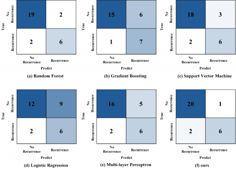
The confusion matrix for the five-year follow-up window is shown in Figure 5. In the test set containing 29 samples, there are 8 recurrence samples and 21 non-recurrence samples. The SDDFF model achieves excellent classification performance. It correctly identifies 20 true negative samples, produces only 1 false positive error, and correctly predicts 2 false negatives and 6 true positives, resulting in Accuracy of 0.897, Precision of 0.857, Recall of 0.750, and F1 of 0.800. Horizontal comparison shows that under similar Recall levels, compared with Random Forest, SVM, MLP, and Logistic Regression, all of which share 2 false negatives, the SDDFF model demonstrates the best false positive control. Although Gradient Boosting has slightly better false negative control, the proposed method does not trade higher Recall for relaxed positive thresholds but maintains comparable detection rates under lower false positives, demonstrating a more balanced performance between Precision and Recall. The confusion matrices for all methods in this fold are shown in Figure 5, with total statistics and fluctuation ranges across folds presented in Table 2.
Table 2. Five-year recurrence prediction comparison
|
Method |
ACC |
Precision |
Recall |
F1 |
|
Random Forest [20] |
0.862± 0.064 |
0.750± 0.153 |
0.750± 0.153 |
0.750± 0.108 |
|
Gradient Boosting [21] |
0.759± 0.079 |
0.538± 0.138 |
0.875± 0.117 |
0.667± 0.111 |
|
Support Vector Machine [22] |
0.828± 0.070 |
0.667± 0.157 |
0.750± 0.153 |
0.706± 0.111 |
|
Logistic Regression [23] |
0.621± 0.090 |
0.400± 0.126 |
0.750±0.153 |
0.522±0.114 |
|
Multi-layer Perceptron [24] |
0.759± 0.079 |
0.545± 0.150 |
0.750± 0.153 |
0.632± 0.114 |
|
SDDFF-Model (Ours) |
0.897± 0.057 |
0.857± 0.132 |
0.750± 0.153 |
0.800± 0.104 |
Figure 5. Five-year recurrence prediction confusion matrix
Figure 6. ROC curve of five-year recurrence experiment
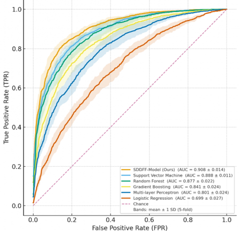
The ROC curve analysis further validates the excellent discriminative ability of the SDDFF model under the five-year follow-up window. As shown in Figure 6, the average curve of the SDDFF model forms an upper envelope over most false positive rate intervals, with an AUC of 0.908±0.014, significantly exceeding SVM (0.888±0.011), Random Forest (0.877±0.022), Gradient Boosting (0.841±0.024), MLP (0.801±0.024), and Logistic Regression (0.699±0.027). Notably, in the clinically more concerned low false positive operating region, when the false positive rate is controlled below 0.10, the SDDFF model can maintain a true positive rate of approximately 0.82, and when the false positive rate is relaxed to 0.20, the true positive rate can further increase to about 0.89. The gray error band clearly shows the standard deviation distribution range across fold mean points, indicating that the curves of all algorithms are generally separated and fluctuations are controllable. This result fully demonstrates that the SDDFF method achieves a more balanced optimization between overall discriminative ability and detection rate in the low false positive operating region, showing good robustness and potential clinical application value.
3.6 Ablation experiment
To further analyze the specific contribution of each component to the overall performance of the SDDFF model, a systematic ablation experiment was designed. The experiment adopts the same data partition, preprocessing workflow, training strategy, and network hyperparameter configuration as the main model to ensure comparability and reliability of the results. The ablation experiment is divided into two levels: the first group compares the effect of branch structures, including only static branch, only dynamic branch, and the complete two-level fusion architecture; the second group verifies the effectiveness of the fusion strategy, covering single-level concatenation, single-level addition, FiLM conditional fusion, and the two-level fusion scheme proposed in this study. The remaining module settings are unchanged, and all metrics are calculated based on stratified five-fold cross-validation, reporting mean and standard deviation. This section focuses on the trend changes of F1, Accuracy, and AUC, with particular analysis of model performance in the low false positive rate region of the ROC curve.
3.6.1 Branch ablation
The quantitative analysis results of the branch ablation experiment reveal the important role of each core component of the SDDFF model (See Table 3). Evaluation based on five-year follow-up test data shows that using only the static branch or dynamic branch exhibits obvious performance limitations. The static branch scheme is relatively stable in overall discriminative ability but has a certain degree of false positive issues; the dynamic branch can improve detection ability, but the false positive rate correspondingly increases. Following the design concept in Section 2.4, the SDDFF model combines vector-level global reliability allocation with feature-level fine-grained weighting through a two-level fusion mechanism, successfully minimizing false positives while maintaining comparable detection rates. Experimental data show that the complete SDDFF model achieves significant improvements in overall metrics compared with single-branch schemes, with Accuracy, Precision, and F1 outperforming both single-branch schemes, verifying the complementary effect of static attributes and longitudinal dynamic signals in recurrence prediction discrimination.
Table 3. Branch structure ablation experiment
|
Method |
ACC |
Precision |
Recall |
F1 |
|
Static Branch Only |
0.828± 0.069 |
0.667± 0.133 |
0.750± 0.153 |
0.706± 0.117 |
|
Dynamic Branch |
0.828± 0.070 |
0.636± 0.113 |
0.875± 0.117 |
0.737± 0.095 |
|
SDDFF-Model (Ours) |
0.897± 0.057 |
0.857± 0.132 |
0.750± 0.153 |
0.800± 0.104 |
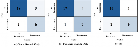
The confusion matrix of the branch ablation experiment visually shows the impact mechanism of different architecture designs on classification performance. From the five-year follow-up test data in Figure 7, it can be clearly observed that the static branch shows relatively balanced performance in overall discriminative ability, but its false positive control is obviously insufficient, with 3 misclassified samples and 2 false negatives. In contrast, the dynamic branch, although more sensitive in detection ability, increases the number of false positives to 4, with true positive predictions rising to 7. The complete SDDFF model, through the carefully designed two-level fusion mechanism, successfully integrates the advantages of both branches, maintaining a true positive detection level comparable to the dynamic branch while controlling false positives to an optimal level of 1. This result fully confirms the model's comprehensive superiority in Accuracy, F1, and Precision, validating the significant complementary effect between single-timepoint static attributes and longitudinal dynamic signals, and showing that the dual-branch fusion architecture achieves a more ideal trade-off between Precision and Recall balance.
Figure 7. Confusion matrix of branch ablation experiment
3.6.2 Ablation of feature fusion module
The ablation experiment of feature fusion strategy further reveals the core value of the two-level fusion mechanism in the SDDFF model (See Table 4). Experimental data show that the three single-level baseline fusion methods all exhibit obvious high false positive issues at moderate detection rate levels. Specifically, the average number of false positives in the Single-Stage Concat and Single-Stage Sum strategies remains around 3, while the FiLM-CF method shows more severe false positives, approximately 4, with an increasing trend of missed detections. In contrast, the Two-Level Fusion architecture of the SDDFF model successfully controls false positives at the ideal level of 1, while achieving excellent performance in Precision, F1, and Accuracy, reaching 0.857, 0.800, and 0.897, respectively. This comparison strongly demonstrates the significant advantage of the "vector-level—feature-level" joint modeling strategy, indicating that, compared with simple single-stage fusion operations, the hierarchical feature integration mechanism can establish a more robust balance between Precision and Recall, providing a more reliable technical solution for recurrence risk prediction tasks.
Table 4. Feature fusion module ablation experiment
|
Method |
ACC |
Precision |
Recall |
F1 |
|
Single-Stage Concat |
0.828± 0.069 |
0.667± 0.133 |
0.750± 0.153 |
0.706± 0.117 |
|
Single-Stage Sum |
0.793± 0.072 |
0.625± 0.150 |
0.625± 0.171 |
0.625± 0.136 |
|
FiLM-CF [25] |
0.759± 0.077 |
0.556± 0.139 |
0.625± 0.171 |
0.588± 0.132 |
|
SDDFF-Model (Ours) |
0.897± 0.057 |
0.857± 0.132 |
0.750± 0.153 |
0.800± 0.104 |
Figure 8. Confusion matrix of fusion ablation experiment
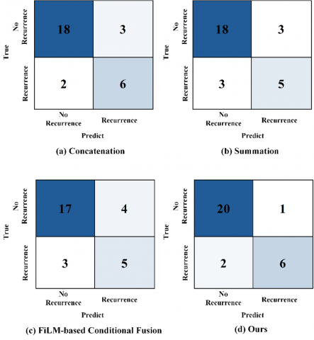
The confusion matrix of the fusion strategy ablation experiment clearly presents the performance differences of different feature integration schemes. Observing the classification results of a representative test fold in the five-year follow-up window in Figure 8, it can be seen that the simple concatenation and addition strategies maintain moderate detection ability, but both face the same false positive control problem, with false positives fixed at 3, resulting in F1 and Accuracy metrics below the expected performance of the fusion scheme. The FiLM conditional fusion strategy, while attempting to improve feature interaction, produces side effects: the number of false positives increases to 4, and missed detections also worsen to 3, failing to achieve the expected performance improvement. The two-level fusion architecture of the SDDFF model demonstrates a completely different optimization effect. Through the joint mechanism of "vector-level global reliability allocation plus feature-level fine-grained weighting," it successfully compresses the number of false positives to the optimal level of 1 while maintaining a comparable detection rate, with Precision, F1, and Accuracy improving to 0.857, 0.800, and 0.897, respectively. The experimental results fully confirm the significant advantage of the adaptive "vector-level—feature-level" joint fusion architecture compared with single fusion strategies in balancing Precision and Recall.
The static–dynamic dual-branch fusion model proposed in this study demonstrated superior performance in post-radiotherapy recurrence prediction, verifying the complementary discrimination ability of static clinical features and longitudinal dynamic features. Compared with traditional methods, this model achieved significant improvements in multiple metrics, including Accuracy, F1, and AUC, especially showing stronger clinical practical value in the low false positive region. Future work will further expand the data scale, explore multimodal fusion of radiomics and dosimetric features, and conduct external validation in multicenter cohorts to enhance the generalizability and applicability of the model, providing stronger support for individualized precision follow-up and decision support.
Appendix I
|
Static Indicators |
|
Sex |
|
Age |
|
Height (m) |
|
Diag |
|
Site |
|
Grade |
|
T |
|
N |
|
M |
|
Stage |
|
Oncologic Treatment Summary |
|
Induction Chemotherapy |
|
Chemotherapy Regimen |
|
Platinum-based chemotherapy |
|
Received Concurrent Chemoradiotherapy |
|
CCRT Chemotherapy Regimen |
|
Surgery Summary |
|
RT Total Dose (Gy) |
|
Dose/Fraction (Gy/fx) |
|
Number of Fractions |
|
Total RT treatment time (days) |
|
Smoking History |
|
Current Smoker |
|
Unplanned Additional Oncologic Treatment |
|
Received Feeding Tube (Y/N) |
|
Type of feeding tube |
|
Feeding tube duration (months) |
|
Time between pre and post image (months) |
|
Time from preRT image to start RT (month) |
|
Time from RT stop to follow up imaging (months) |
Appendix II
|
Dynamic Indicator |
|
BW tx (kg) |
|
BMI start treat (kg/m2) |
|
RT L3 Skeletal Muscle Cross Sectional Area (cm2) |
|
RT L3 Adipose Tissue Cross Sectional Area (cm2) |
|
RT L3 Skeletal Muscle Index (cm2/m2) |
|
RT L3 Adiposity Index (cm2/m2) |
|
RT CT-derived lean body mass (kg) |
|
RT CT-derived fat body mass (kg) |
|
RT Skeletal Muscle status |
[1] Johnson, D.E., Burtness, B., Leemans, C.R., Lui, V.W.Y., Bauman, J.E., Grandis, J.R. (2020). Head and neck squamous cell carcinoma. Nature Reviews Disease Primers, 6(1): 92. https://doi.org/10.1038/s41572-020-00224-3
[2] Sung, H., Ferlay, J., Siegel, R.L., Laversanne, M., Soerjomataram, I., Jemal, A., Bray, F. (2021). Global cancer statistics 2020: GLOBOCAN estimates of incidence and mortality worldwide for 36 cancers in 185 countries. CA: A Cancer Journal for Clinicians, 71(3): 209-249. https://doi.org/10.3322/caac.21660
[3] Pannunzio, S., Di Bello, A., Occhipinti, D., Scala, A., Messina, G., Valente, G., Cassano, A. (2024). Multimodality treatment in recurrent/metastatic squamous cell carcinoma of head and neck: Current therapy, challenges, and future perspectives. Frontiers in Oncology, 13: 1288695. https://doi.org/10.3389/fonc.2023.1288695
[4] Zhang, Q., Wang, K., Zhou, Z., Qin, G., Wang, L., Li, P., Wang, J. (2022). Predicting local persistence/recurrence after radiation therapy for head and neck cancer from PET/CT using a multi-objective, multi-classifier radiomics model. Frontiers in Oncology, 12: 955712. https://doi.org/10.3389/fonc.2022.955712
[5] Wong, E.T., Dmytriw, A.A., Yu, E., Waldron, J., Lu, L., Fazelzad, R., Huang, S.H. (2019). 18F-FDG PET/CT for locoregional surveillance following definitive treatment of head and neck cancer: A meta-analysis of reported studies. Head & Neck, 41(2): 551-561. https://doi.org/10.1002/hed.25513
[6] Baxi, S.S., Dunn, L., Pfister, D.G. (2015). Evaluating the potential role of PET-CT in the post-treatment surveillance of head and neck cancer. Journal of the National Comprehensive Cancer Network: JNCCN, 13(3): 252-254. https://doi.org/10.6004/jnccn.2015.0036
[7] Beesley, L.J., Hawkins, P.G., Amlani, L.M., Bellile, E.L., Casper, K.A., Chinn, S.B., Taylor, J.M. (2019). Individualized survival prediction for patients with oropharyngeal cancer in the human papillomavirus era. Cancer, 125(1): 68-78. https://doi.org/10.1002/cncr.31739
[8] Ang, K.K., Harris, J., Wheeler, R., Weber, R., Rosenthal, D.I., Nguyen-Tân, P.F., Gillison, M.L. (2010). Human papillomavirus and survival of patients with oropharyngeal cancer. New England Journal of Medicine, 363(1): 24-35. https://doi.org/10.1056/NEJMoa0912217
[9] Vallieres, M., Kay-Rivest, E., Perrin, L.J., Liem, X., Furstoss, C., Aerts, H.J., El Naqa, I. (2017). Radiomics strategies for risk assessment of tumour failure in head-and-neck cancer. Scientific Reports, 7(1): 10117. https://doi.org/10.1038/s41598-017-10371-5
[10] Lv, W., Ashrafinia, S., Ma, J., Lu, L., Rahmim, A. (2019). Multi-level multi-modality fusion radiomics: Application to PET and CT imaging for prognostication of head and neck cancer. IEEE Journal of Biomedical and Health Informatics, 24(8): 2268-2277. https://doi.org/10.1109/JBHI.2019.2956354
[11] Bogowicz, M., Riesterer, O., Ikenberg, K., Stieb, S., Moch, H., Studer, G., Tanadini-Lang, S. (2017). Computed tomography radiomics predicts HPV status and local tumor control after definitive radiochemotherapy in head and neck squamous cell carcinoma. International Journal of Radiation Oncology* Biology* Physics, 99(4): 921-928. https://doi.org/10.1016/j.ijrobp.2017.06.002
[12] Li, M., Jiang, Y., Zhang, Y., Zhu, H. (2023). Medical image analysis using deep learning algorithms. Frontiers in Public Health, 11: 1273253. https://doi.org/10.3389/fpubh.2023.1273253
[13] Zhou, S.K., Greenspan, H., Davatzikos, C., Duncan, J.S., Van Ginneken, B., Madabhushi, A., Summers, R.M. (2021). A review of deep learning in medical imaging: Imaging traits, technology trends, case studies with progress highlights, and future promises. Proceedings of the IEEE, 109(5): 820-838. https://doi.org/10.1109/JPROC.2021.3054390
[14] Takada, T., Tambas, M., Clementel, E., Leeuwenberg, A., Sharabiani, M., Schuit, E. (1996). Prognostic models for radiation-induced complications after radiotherapy in head and neck cancer patients. Cochrane Database of Systematic Reviews, 2025(9): CD014745. https://doi.org/10.1002/14651858.CD014745
[15] Iorio, G.C., Denaro, N., Livi, L., Desideri, I., Nardone, V., Ricardi, U. (2024). Editorial: Advances in radiotherapy for head and neck cancer. Frontiers in Oncology, 14: 1437237. https://doi.org/10.3389/fonc.2024.1437237
[16] Parker, M.I., Su, W.W., Kang, M., Yuan, Y., Gupta, V., Liu, J.T., Bakst, R.L. (2024). Deep learning based recurrence prediction in head and neck cancers after radiotherapy. International Journal of Radiation Oncology, Biology, Physics, 118(5): e65. https://doi.org/10.1016/j.ijrobp.2024.01.146
[17] Yang, H., Yang, M., Chen, J., Yao, G., Zou, Q., Jia, L. (2025). Multimodal deep learning approaches for precision oncology: A comprehensive review. Briefings in Bioinformatics, 26(1): bbae699. https://doi.org/10.1093/bib/bbae699
[18] Mansouri, Z., Salimi, Y., Amini, M., Hajianfar, G., Oveisi, M., Shiri, I., Zaidi, H. (2024). Development and validation of survival prognostic models for head and neck cancer patients using machine learning and dosiomics and CT radiomics features: A multicentric study. Radiation Oncology, 19(1): 12. https://doi.org/10.1186/s13014-024-02409-6
[19] Grossberg, A.J., Mohamed, A.S., Elhalawani, H., Bennett, W.C., Smith, K.E., Nolan, T.S., Fuller, C.D. (2018). Imaging and clinical data archive for head and neck squamous cell carcinoma patients treated with radiotherapy. Scientific Data, 5: 180173. https://doi.org/10.1038/sdata.2018.173
[20] Breiman, L. (2001). Random forests. Machine Learning, 45(1): 5-32. https://doi.org/10.1023/A:1010933404324
[21] Friedman, J.H. (2001). Greedy function approximation: a gradient boosting machine. The Annals of Statistics, 29(5): 1189-1232.
[22] Cortes, C., Vapnik, V. (1995). Support-vector networks. Machine Learning, 20(3): 273-297.
[23] Hosmer Jr, D.W., Lemeshow, S., Sturdivant, R.X. (2013). Applied logistic regression. New York, NY, USA: Wiley.
[24] Rumelhart, D.E., Hinton, G.E., Williams, R.J. (1986). Learning representations by back-propagating errors. Nature, 323(6088): 533-536. https://doi.org/10.1038/323533a0
[25] Perez, E., Strub, F., De Vries, H., Dumoulin, V., Courville, A. (2018). FiLM: Visual reasoning with a general conditioning layer. Proceedings of the AAAI Conference on Artificial Intelligence, 32(1): 3942-3951. https://doi.org/10.1609/aaai.v32i1.11671