Majid Roohi![]() | Jalil Mazloum*
| Jalil Mazloum*![]() | Mohammad A. Pourmina
| Mohammad A. Pourmina![]() | Behbod Ghalamkari
| Behbod Ghalamkari![]()
© 2025 The authors. This article is published by IIETA and is licensed under the CC BY 4.0 license (http://creativecommons.org/licenses/by/4.0/).
OPEN ACCESS
Stroke is a leading cause of death, especially among the elderly. Early diagnosis and treatment are crucial. This research uses a microwave brain imaging system with circular array antennas and a multilayer head phantom to detect 1 cm spherical targets. Signal processing techniques, like averaging and beamforming, are employed to improve image quality in the desired band (0.5-6 GHz). To classify stroke types, a deep learning approach is applied. Reconstructed images are fed into a multiclass linear SVM trained with CNN features extracted using residual learning. The proposed method accurately locates bleeding targets with a 97% success rate and effectively distinguishes between different stroke types.
brain stroke classification, microwave head imaging system, confocal image reconstruction algorithm, intracranial hemorrhage stroke detection, CNN, SVM classifier
Traditional methods of stroke diagnosis, such as computed tomography (CT) scans and MRI, face limitations in accessibility, sensitivity, interpretation, invasiveness, and speed. These limitations can delay timely treatment and hinder accurate diagnosis, potentially worsening patient outcomes. Emerging technologies like optical coherence tomography, near-infrared spectroscopy, and biomarkers hold promise for rapid, non-invasive, and portable stroke assessment. Artificial intelligence and machine learning techniques can enhance scan interpretation and personalize treatment plans, while boosting the time required for diagnosis and increase its accuracy. Combining modalities and integrating translational research will accelerate the development and implementation of improved diagnostic approaches for stroke [1-5]. Recently, microwave imaging systems (MIS) is considered as a portable brain scan system [1-5]. The brain MIS objective is detection of cancerous tumors, ischemic or hemorrhage caused by brain injuries, and brain activity surveillance [1, 2]. For this system several main factors significantly affect the imaging performance, e.g., the antenna dimension and its radiation characteristics, image reconstruction methods, post-processing techniques. Several imaging methods used in medical imaging systems were proposed [1-3]. Generally, imaging methods are classified in two main quantitative and qualitative categories. Quantitative methods such as tomography, dielectric constant and region of interest (ROI) are extracted based on recursive methods. The images reconstructed by these methods are time consuming, but has a good spatial resolution. In contrary, qualitative methods, e.g., radar-based methods, are founded on reflection signal delays. As these methods are faster than qualitative methods, these are adopted as real time methods, more suitable for hospital adoption. Machine learning techniques, which are used in MIS, are highly capable of segmentation, clustering and classification [6-15]. A neural network with microwave imaging for a complex data collection forward learning machine is compounded [8]. Additionally, Rekanos [9] have proposed a radial based neural network for proliferated brain position and size estimation into skeleton tissue with microwave imaging. Li et al. [10] have adopted a deep neural network for enhancing the created image. Their deep neural network had been trained to obtain a much better image from created microwave images using the back-projection method as input. Efforts have been made to address the nonlinear electromagnetic inverse problem through iterative techniques. Recently, studies have explored the use of deep learning methods to enhance 2D microwave imaging for breast examinations [11]. Radar-based approaches have also been employed by researchers to investigate machine learning applications in diagnosing breast lesions [12]. Wan et al. [13] introduced an innovative classification technique for automatic diagnosis derived from reconstructed images using microwave tomography. This approach can aid in identifying cancerous tumors within breast tissue. In microwave imaging tomography systems, image reconstruction is based on the characteristics of the dielectric environment. Another classification is founded directly on signal characteristics, without dielectric characteristic reconstruction. E.g., Nanni et al. [15] introduced a novel approach to categorizing intracervical hemorrhage in relation to ischemic stroke. Where the benefits of adopting deep learning for diagnosis and classification of two brain strokes types in the accurate full head phantom model, in multi-static MIS are investigated. The primary objective of this study is to develop and validate a novel deep learning-based classification method to distinguish between ischemic and hemorrhagic strokes using multi-static MIS. Thus, a circular shaped matrix of butterfly antennas is placed around the unhealthy head, so that 0.5 to 6 GHz are covered. Reflected signals are collected by different multi-static channels, then these are used as inputs to the confocal imaging reconstructing algorithm for mapping extracted information in the 2D image. Due to the importance of clustering in distinguishing hemorrhage from ischemic stroke, a new hybrid post-processing method is applied during ROI image creation. Therefore, feature extraction using conventional neural network (CNN) is implemented. Then, support vector machine (SVM) clustering is adopted. One of the challenges is to setup the test setup consisting of the artifact, beam forming and post-processing methods in a MIS. This research aims to address limitations in current diagnostic methods by leveraging innovative machine learning techniques and enhancing the efficacy of MIS for rapid, non-invasive, and precise stroke diagnosis. The proposed imaging system results indicate that using the proposed deep learning method can distinguish the two types of stokes mentioned in radar-based images exhibit significant ambiguity.
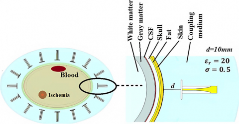
Here the brain microwave imaging scenario for connecting deep learning approaches and proving its effectiveness for stroke classification is described. The microwave-simulated brain imaging scenario is depicted in Figure 1; for further information and a description, readers are referred to the study [16]. Realization of microwave brain imaging scenario consists of three main levels. From bottom-up, at the first level, 16 antennas are placed around the full phantom, irradiating electromagnetic waves in the frequency range of 0.5 to 6 GHz. At the next layer, the confocal image reconstruction algorithm is situated, which can minimize the reflected wave from the skin at the head phantom border. A suitable matching medium between the antennas and head phantom is also designed. This special layer can help to increase the penetration depth of the transmitted wave inside the head phantom.
Figure 1. Design and arrangement of antennas in microwave brain imaging
As shown in Figure 1, to realize the proposed imaging system, a multi-layer human head phantom model is created in CST software [17]. For ease of modeling and imaging, the head phantom includes all human head anatomical details from the skin layer to the white matter of the brain. All phantom head material electrical characteristics used are given in Table 1. In addition, as seen in Figure 1, sixteen proposed antennas encircling the head at equal distances of 10 mm from the skin layer and a bleeding stroke located inside the head are used in the model.
Table 1. Different brain layers electrical characteristics [16]
|
Layer |
Depth (mm) |
r (mm) |
R (mm) |
|
Skin |
2 |
80 |
120 |
|
Fat |
1.4 |
78 |
118 |
|
Skull |
4.1 |
76.6 |
116.6 |
|
Cerebrospinal fluid |
0.5 |
73.4 |
113.4 |
|
Grey matter |
7 |
72.9 |
112.9 |
|
White matter |
Inner part |
65 |
105 |
|
Blood |
10 |
10 |
- |
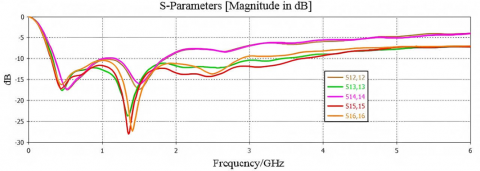
Designing an appropriate propagation framework that includes the antenna, matching medium, and brain model is an important step in setting up microwave brain imaging. In this paper, the mismatch effects between the antenna and the head phantom are reduced by shielding the antennas in a well-designed matching medium [18]. The simulation model used is the multi-static model. In other words, there is only one transmitter antenna and one active receiver antenna in each stage, so there are no received signal wave interactions for the side antennas. To ensure electrical matching between the antennas and the area under test, a transmission medium is designed based on electrical characteristics parametric sweep. The electrical characteristics calculated for this medium are $\varepsilon_r$=20 and $\sigma$=0.5 S/m. Five proposed antenna simulated reflected signal characteristic examples at different positions within the designed matching medium are shown in Figure 2. It can be seen that, with a suitable matching medium permittivity and conductivity, all sixteen antennas radiate from 0.5 to 6 GHz.
Figure 2. Five proposed antenna simulated reflected signal characteristic examples inside the designed
In the present section, it is shown that MIS based on radar can be adopted for stroke detection using confocal imaging algorithm and the results are analyzed. It is clear that detecting hemorrhage related to stroke is of utmost importance and is necessarily considered in real time. Thus, after simulation and setting up the designed imaging system, all reflected signals are stored in MATLAB for image reconstruction. This process consists of three main parts; pre-processing, processing, and post-processing. The main objective at the pre-processing stage is to calibrate the reflected signals and eliminate clutter. The processing stage coherently integrates the data based on delay-and-sum (DAS) algorithm. Finally, at post-processing the deep learning algorithm is adopted to determine the stroke type.
As stated, the first stage for image creation for all imaging algorithms is to calibrate the obtained signals or skin artifact removal.
Next, two calibration methods, ideal subtraction and averaging methods, are presented.
3.1 Ideal subtraction method
Ideal subtraction method is a difference calibration method used for removing background by modeling healthy and unhealthy tissues. Then, the reflected signals are subtracted with regard to each other and the calibrated signals will be obtained as Eq. (1) [19]:
$s_m=x_m^{\text {with}}-x_m^{\text {without}}$ (1)
3.2 Averaging method
The averaging method removes the skin artifact by obtaining the average signal emanating from all channels, then this signal is deducted from each channel. For instance, not considering skin artifact for the signal in the mth channel yields [19]:
$s_m(n)=x_m(n)-\frac{1}{M} \sum_{i=1}^M x_i(n)$ (2)
where, $s_m$ is the signal without the skin artifact, M is the number of signals, and n is the sample counter.
To create an image based on the obtained signals from the first stage, the confocal image reconstruction algorithm DAS and an improved beamformer called as delay-multiply-and-sum (DMAS) is used [20]. Both beamformers work with a slight difference based on the reflected signal displacement in real time to create a correlated signal.
3.3 DAS beamformer
To implement confocal image reconstruction algorithm with M antennas and considering $S_n$ as the ith reflected signal, the energy at each focal position r can be expressed as Eq. (3):
$I(r)=\int_0^{T_w}\left[\sum_{i=1}^M S_n\left(t-\tau_i(r)\right)\right]^2 d t, r=[x ; y ; z]$ (3)
where, $T_w$ is the window length, $T_s$ distance to sample, and $\tau_i(r)$, the ith discrete time delay, that can be calculated as Eq. (4):
$\tau_i(r)=\frac{2 d_i(r)}{v T_s}$ (4)
For which, $v$ is the average wave propagation speed in the brain medium and $d_i(r)$ is the discrete time distance between the ith displacement antenna, $r_n$, to $r$.
$d_i(r)=\left|r-r_i\right|$ (5)
In a multi-static system $M^2$ signals can be recorded, but for calculating the energy characteristics, only $M(M-1) / 2$ signals are needed.
3.4 DMAS beamformer
Another useful beamformer for confocal image reconstruction algorithm is the DMAS beamformer [21]. It consists of multiplied and summed time modified signals, similar to DAS, which are used to calculate the energy at a focal point. The energy at r inside the brain is defined as follows.
$I(r)=\int_0^{T_w}\left[\sum_{i=1}^{M-1} \sum_{j=n+1}^M S_n\left(t-\tau_i(r)\right) S_j\left(t-\tau_j(r)\right)\right]^2 d t$ (6)
For which, $M$ is the number of antennas used for multi-static imaging. In confocal image reconstruction method, the image pixel intensity (brightness) at the nth cell region and direction, $\theta$, are related as $F_i(n)$.
$F_i(n)={ }_{n=1}^N f_i X_i(n) e^{j \phi_i}$ (7)
In Eq. (7), $X_i(n)$ is the received signal from the ith antenna and N is the total number of receiving antennas. Further, to consider medium effects, propagation damping and loss, $f_i$ is added as a weight parameter. To compensate the phase difference due to different paths, $\varphi_i$ is used [22]. In the present work, it is assumed that the wave is propagating in a spherical front inside the brain medium.
Table 2. Comparison of selected calibration and beamformer methods with quality factor metrics
|
Calibration |
Beamformer |
$\delta$ (mm) |
SCR (dB) |
SMR (dB) |
|
Ideal subtraction |
DAS |
4 |
0.97 |
10.86 |
|
DMAS |
3 |
0.98 |
10.93 |
|
|
Averaging method |
DAS |
4.5 |
0.87 |
9.1 |
|
DMAS |
3.8 |
0.9 |
9.24 |
|
|
Ideal subtraction and Averaging method |
DAS |
3.5 |
1.2 |
11.1 |
|
DMAS |
2 |
1.5 |
11.5 |
A comparison between pre-processing and processing algorithms by quality factor metrics is made. First, the signals are passed from the ideal subtraction method and then the averaging method, mentioned above. Later, the DAS and DMAS algorithms are used to determine the energy levels. A white Gaussian noise with signal to noise ratio (SNR) 10dB is added to the reflected signals. The evaluation regions are two displaced 20 mm diameter spherical strokes. As shown in Figure 1, one subject is a hemorrhage stroke and the other a vein clogging or an ischemic. Both are located at the same height, i.e. z = 0. The hemorrhage is located at x = 10, y = 60 and the ischemic at x = -30, y = -45. The post-processing parameters for the hemorrhage of interest are presented in Table 2. To compare algorithm performances, the following criteria are considered.
3.5 Quality factor
To express obtained image quality or, in other words, evaluating the imaging performance quality factors are used. Generally, signal to mean ratio (SMR) and signal to clutter ratio (SCR) parameters are used.
SMR is the ratio of the highest reflected energy in the tumor $\left(r e c_T\right)$ to the average model energy ( $r e c_{T. \text {ave}}$ ), expressed as Eq. (8) [23].
$S M R=10 \log \frac{\max \left(r e c_T\right)}{r e c_{\text {T.ave }}}$ (8)
SCR is the ratio of the highest reflected energy in the tumor $\left(r e c_T\right)$ to the maximum energy at other locations $\left(\mathrm{rec}_T^{\prime}\right)$, expressed as Eq. (9) [23].
$S C R=10 \log \frac{\max \left(r e c_T\right)}{r e c_T^{\prime}}$ (9)
With the above definitions, the tumor is correctly assessed when SMR and SCR values are larger than 10 dB and 0 dB, respectively.
With the results presented in the above table, the subtraction calibration method is selected due to simplicity, high speed, and creation of suitable images for the post-processing stage. Finally, to increase the difference between the subject and background or, with other words, reducing clutter effects, and also removing multiple reflections and background clutter residuals the averaging method is adopted. During the processing stage, initially DAS beamformer and then DMAS is adopted to improve the outcome. Although these beamformers are simple, they are very powerful at concentrating energy at the focal points. As the received signal clarity from the calibration stage is suitable, using the mentioned beamformers, will offer high quality images to the post-processing stage.
One main challenge in designing deep learning methods for brain MIS, is to diagnose the stroke type. This challenge can be related to the reconstructed image from the received signals. To address this issue, a combination of CNN method for feature extraction and SVM classification method has been used as a classifier.
In the present section, the stroke type classification method for brain MIS based on CNNs and SVM is presented. Also, in this approach, the definition of residual neural network (ResNet) has been used. ResNet is an artificial neural network based on the known structures of pyramidal cells in the cerebral cortex. ResNet has recently gained popularity due to its great image recognition performance. The considered specific approach is based on residual mapping which allows to achieve better results also in the training phase [24]. In particular, ResNet models are based on connections/shortcuts that allows for traversing certain layers. Typical models of this network are implemented with two- or three-layer skips containing nonlinearities and batch normalization.
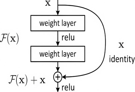
The main residual learning block with skip connection is shown in Figure 3. ResNet architecture is suitable for image classification, regression, and feature extraction. This architecture uses skip connections to add a group of convolution inputs to its output. The "skip connection" shown in Figure 3 is the core of the ResNet implementation, which is the idea of building a network of branches with skip connections. For each branch, the difference, residual activation map between input and output in each branch, is trained by the algorithm. This residual activation map is aggregated with previous activation maps to form the "collective knowledge" of ResNet. Deeper neural network training has historically been difficult. Residual learning with skip connections enables the training of deeper models than ever before, resulting in high-performance networks with more than 1000 layers. For most recent models, it is observed that deeper models are more powerful. This detection map has no parameters and is only used to add the output from the previous layer to the next layer. However, sometimes $x$ and $F(x)$ will not have the same dimensions. The identity mapping or recognition map is multiplied by a linear mapping factor $W$ to expand the shortcut channels to match the remainder [25]. This allows $x$ and $F(x)$ to be combined as input to the next layer.
$y=F\left(x,\left\{W_i\right\}\right)+W_s x$ (10)
Figure 3. Residual learning structure with skip connection [26]
Eq. (10) is used as $x$ and $F(x)$ have different dimensions, e.g., $32 \times 32$ and $30 \times 30 . W_s$ can be implemented to introduce additional parameters with a $1 \times 1$ convolution to the model.
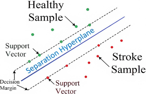
In this work, the feature extracted from ResNet is used as input in SVM. SVM is defined as the linear classifier with the largest distance in the feature space [27]. The main process in SVM is to find an optimal hyperplane in the feature space that maximizes the classification features. The concept of maximum margin with bounding planes and support vectors is shown in Figure 4. The decision boundary as the centerline can be defined by a normal vector of the hyperplane and an offset by Eq. (11), as shown in Figure 4.
Figure 4. Concept of maximum margin with bounding planes in SVM classification
$f(x)=w_T x+b$ (11)
In this paper, the main goal is to identify healthy tissue from stroke samples, which is a three-class problem. Consider the three-class discriminant training dataslet problem, a feature vector, $Z^i \in R_k$, and the class label, $y_i \in-1,+1$. If each of the classes are assumed to be separated by a hyperplane as Eq. (12) in the given space H.
$w z+b=0$ (12)
The performance of the classification decision function can be written as follows:
$f(z)=\operatorname{sign}(w z+b)$ (13)
Therefore, the optimal hyperplane maximizes the margin γ:
$\gamma=\frac{y f(z)}{\|w\|}$ (14)
This optimization problem is defined as Eq. (15).
$\max _{w, b} \gamma \operatorname{st} y_i f\left(z^i\right)>1$ (15)
The optimal values for $w$ and $b$ can be obtained by solving a minimization problem using the Lagrange coefficient. For the training set, the feature vectors extracted from the CNN are used to structure the SVM classification. Then some of them are used for the test set, which aids in evaluating the SVM classifier.
Next, the details of the CNN-SVM hybrid method will be reviewed. Specifically, the proposed method includes a pre-trained CNN, used as a feature extractor for image classification training. CNNs are trained using three image set categories including natural or healthy, ischemic and bleeding or hemorrhagic. CNNs can be trained with robust examples representing a range of images using these collections [27]. An easy way to harness the power of CNN, without spending time and effort on training, is to use a pre-trained CNN as a feature extractor.
Based on the aforementioned framework, the first stage is to load the test image. Then, by using CNN to extract a series of features, the processing speed and classification are improved. Based on these inputs, the main challenge is to determine the weight of the convolution layers. To simulate bleeding targets, blood-like substances have been used. While ischemic targets are modeled with materials having an electrical permeability 15% lower than blood.
This classification method extracts a feature vector from each image, on which the classification is made. Specific images are simulated based on different scenarios. The ResNet-50 model has also been used for CNN from deep learning toolbox in MATLAB [28]. After loading the reconstructed images in MATLAB, they are labeled according to the corresponding image types, the number of these categories are shown in Table 3 along with the number of image samples in each category.
Table 3. Input image labels
|
Label |
Number |
|
Normal tissue (healthy) |
11 |
|
Hemorrhagic stroke |
7 |
|
Ischemic stroke |
8 |
Different stroke types are defined for each classification group to assess the stroke type for each input image. The program is automated; the test image is taken as an input, then the neural network algorithm is used through deep learning to extract each image feature. The neural network proposed in this study uses the "fc1000" class capable of detecting edges and spots to extract features. In the designed CNN configuration, the first convolution layer is weighted according to the input image. The extracted features are used as inputs to the SVM classification program. Some of these features are used for training (70%) and others for testing (30%) the classification program. A multi-class SVM program is used for classification.
To evaluate the proposed method, a confusion matrix was created (presented as Table 4) based on the three labels of Table 3. The normalized predicted and actual results are presented as the rows and columns of Table 4, respectively. As the predicted and actual labels have a 1 to 1 correspondence, it can be concluded that the proposed method shows a good detection performance, as the system has a low detection error among different classes. There is only a small discrepancy for the third category, which can be solved by adding more related training samples. The proposed algorithm is able to optimally separate normal tissue and stroke. There is an error in separating the ischemic and hemorrhagic strokes, which is due to the small difference between the electrical conductivity of the two stroke types. To reduce error (improve separation accuracy), a large number of samples per category is needed.
Table 4. Confusion matrix
|
|
Actual Labels |
|||
|
Normal Tissue |
Hemorrhagic Stroke |
Ischemic Stroke |
||
|
Predicted labels |
Normal tissue |
1 |
0 |
0 |
|
Hemorrhagic stroke |
0 |
1 |
0 |
|
|
Ischemic stroke |
0 |
0.337 |
0.667 |
|
Table 5. Proposed method comparison with other similar published articles
|
Method |
Classification |
Number of Features Extracted |
SNR Level (dB) |
Time (s) |
CPU Specification |
|
Proposed method |
97% |
1000 |
21 |
9 |
core i7 @ 1.8 GHz |
|
[11] |
96.1% |
3 |
noiseless |
31 |
not mentioned |
|
[29] |
88% |
3 |
10 and 25 and 45 |
10 |
core i7 @ 3.4 GHz |
To evaluate the classifier performance, a comparison has been made with other recently published articles, presented in Table 5. It can be seen that the proposed method has comparable performance as compared to other methods. The proposed method is not only more accurate, but the overall parameter performances, such as processing time (which plays an essential role), small number of samples needed, simpler feature vector, and most importantly, the sample preparation, leading to the development of a specialized database, also excel. It should be noted that if the number of images is combined with other imaging methods and the number of samples increases, the detection accuracy can be higher than 97% [16]. This accuracy can also be improved by adding to the number of input images, which can be hard to acquire. Therefore, it can be concluded that the proposed method is suitable to classify brain image objects using microwave technology. The algorithm was performed using the MATLAB R2019b tool on a 3.60 GHz IntelR Core™ i7 processor running Windows 10 Enterprise 64-bit operating system, having a 7856MB NVIDIA graphics processing unit.
The main objective of this investigation was to classify stroke types in reconstructed images from a microwave brain imaging system. Thus, a method based on deep learning is presented for predicting the stroke type. Specifically, the proposed method consists of pre-trained CNN and classifying SVM. The approach of this paper is promising and the classification is made accurately and quickly for MISs. It is proposed to implement this technique with other machine leaning methods, e.g. genetic algorithm, to increase its accuracy. Further, other scenarios resulting in more complex biologic tissue modeling can be considered.
[1] Scapaticci, R., Tobon, J., Bellizzi, G., Vipiana, F., et al. (2018). Design and numerical characterization of a low-complexity microwave device for brain stroke monitoring. IEEE Transactions on Antennas and Propagation, 66(12): 7328-7338. https://doi.org/10.1109/TAP.2018.2871266
[2] Sohani, B., Tiberi, G., Ghavami, N., Ghavami, M., et al. (2019). Microwave imaging for stroke detection: Validation on head-mimicking phantom. PhotonIcs & Electromagnetics Research Symposium-Spring (PIERS-Spring), Rome, Italy, pp. 940-948. https://doi.org/10.1109/PIERS-Spring46901.2019.9017851
[3] Wang, J.K., Jiang, X., Peng, L., Li, X.M., et al. (2019). Detection of neural activity of brain functional site based on microwave scattering principle. IEEE Access, 7: 13468-13475. https://doi.org/10.1109/ACCESS.2019.2894128
[4] Ilja, M., Massa, A., Vrba, D., Fiser, O., et al. (2019). Microwave tomography system for methodical testing of human brain stroke detection approaches. International Journal of Antennas and Propagation, 2019: 1-9. https://doi.org/10.1155/2019/4074862
[5] Santorelli, A., Porter, E., Kirshin, E., Liu, Y.J., et al. (2014). Investigation of classifiers for tumor detection with an experimental time domain breast screening system. Progress In Electromagnetics Research, 144: 45-57. https://doi.org/10.2528/PIER13110709
[6] Pokorny, T., Tesarik, J. (2019). Microwave stroke detection and classification using different methods from MATLAB’s classification learner toolbox. European Microwave Conference in Central Europe (EuMCE), Prague, Czech Republic, pp. 500-503.
[7] Conceicao, R.C., O'Halloran, M., Glavin, M., Jones, E. (2010). Support vector machines for the classification of early-stage breast cancer based on radar target signatures. Progress in Electromagnetics Research B, 23: 311-327. https://doi.org/10.2528/PIERB10062407
[8] Rahama, Y.A., Aryani, O.A., Din, U.A., Awar, M.A., et al. (2018). Novel microwave tomography system using a phased-array antenna. IEEE Transactions on Microwave Theory and Techniques, 66: 5119-5128. https://doi.org/10.1109/TMTT.2018.2859929
[9] Rekanos, I.T. (2002). Neural-network-based inverse-scattering technique for online microwave medical imaging. IEEE Transactions Magn, 38: 1061-1064. https://doi.org/10.1109/20.996272
[10] Li, L., Wang, L.G., Teixeira, F.L., Liu, C., et al. (2019). DeepNIS: Deep neural network for nonlinear electromagnetic inverse scattering. IEEE Transactions Antennas Propagation, 67: 1819-1825. https://doi.org/10.1109/TAP.2018.2885437
[11] Chaplot, S., Patnaik, L.M., Jagannathan, N.R. (2006). Classification of magnetic resonance brain images using wavelets as input to support vector machine and neural network. Biomedical Signal Processing and Control, 1: 86-92. https://doi.org/10.1016/j.bspc.2006.05.002
[12] Rana, S.P., Dey, M., Tiberi, G., Sani, L.,et al. (2019). Machine learning approaches for automated lesion detection in microwave breast imaging clinical data. Scientific Reports, 9(1): 10510. https://doi.org/10.1038/s41598-019-46974-3
[13] Wan, X., Qi, M., Chen, T., Cui, T.J. (2016). Field-programmable beam reconfiguring based on digitally-controlled coding meta surface. Scientific Reports, 6(1): 20663. https://doi.org/10.1038/srep20663
[14] Klautau, A., Batista, P., González-Prelcic, N., Wang, Y., et al. (2018). 5G MIMO data for machine learning: Application to beam-selection using deep learning. Information Theory and Applications Workshop (ITA), San Diego, CA, USA, pp. 1-9. https://doi.org/10.1109/ITA.2018.8503086
[15] Nanni, L., Ghidoni, S., Brahnam, S. (2017). Handcrafted vs. non-handcrafted features for computer vision classification. Pattern Recognition, 71: 158-172. https://doi.org/10.1016/j.patcog.2017.05.025
[16] Roohi, M., Mazloum, J., Pourmina, M.A., Ghalamkari, B. (2021). Machine learning approaches for automated stroke detection, segmentation, and classification in microwave brain imaging systems. Progress in Electromagnetics Research C, 116: 193-205. https://doi.org/10.2528/PIERC21080404
[17] CST Studio Suite. Electromagnetic Field Simulation Software, 2024. http://cst.com.
[18] Ojaroudi, M., Bila, S., Salimi, M. (2019). A novel approach of brain tumor detection using miniaturized high-fidelity UWB slot antenna array. In 2019 13th European Conference on Antennas and Propagation (EuCAP), Krakow, Poland, pp. 1-5.
[19] Elahi, M.A., Glavin, M., Jones, E., O'Halloran, M. (2013). Artifact removal algorithms for microwave imaging of the breast. Progress In Electromagnetics Research, 141: 185-200. https://doi.org/10.2528/PIER13052407
[20] Benny, R., Anjit, T.A., Mythili, P. (2020). An overview of microwave imaging for breast tumor detection. Progress In Electromagnetics Research B, 87: 61-91. https://doi.org/10.2528/PIERB20012402
[21] Islam, M.T., Islam, M.T., Samsuzzaman, M., Kibria, S., et al. (2021). Microwave breast imaging using compressed sensing approach of iteratively corrected delay multiply and sum beamforming. Diagnostics, 11: 470. https://doi.org/10.3390/diagnostics11030470
[22] Islam, M.S., Islam, M.T., Hoque, A., Islam, M.T., et al. (2021). A portable electromagnetic head imaging system using metamaterial loaded compact directional 3D antenna. IEEE Access, 9: 50893-50906. https://doi.org/10.1109/ACCESS.2021.3069712
[23] Guo, X., Casu, M.R., Graziano, M., Zamboni, M. (2014). Simulation and design of an UWB imaging system for breast cancer detection. Integration, 47(4): 548-559. https://doi.org/10.1016/j.vlsi.2014.02.001
[24] Qomariah, D.U.N., Tjandrasa, H., Fatichah, C. (2019). Classification of diabetic retinopathy and normal retinal images using CNN and SVM. In 12th International Conference on Information & Communication Technology and System (ICTS), Surabaya, Indonesia, pp. 152-157. https://doi.org/10.1109/ICTS.2019.8850940
[25] Shao, W., Du, Y. (2020). Microwave imaging by deep learning network: Feasibility and training method. IEEE Transactions on Antennas and Propagation, 68: 5626-5635. https://doi.org/10.1109/TAP.2020.2978952
[26] Ghaffari, M., Sowmya, A., Oliver, R. (2019). Automated brain tumor segmentation using multimodal brain scans: A survey based on models submitted to the BraTS 2012-2018 challenges. IEEE Reviews in Biomedical Engineering, 68: 5626-5635. https://doi.org/10.1109/RBME.2019.2946868
[27] Kerhet, A., Raffetto, M., Boni, A., Massa, A. (2006). A SVM-based approach to microwave breast cancer detection. Engineering Applications of Artificial Intelligence, 19: 807-818. https://doi.org/10.1016/j.engappai.2006.05.010
[28] Wu, Y., Zhu, M., Li, D., Zhang, Y., et al. (2016). Brain stroke localization by using microwave-based signal classification. In International Conference on Electromagnetics in Advanced Applications (ICEAA), Cairns, QLD, Australia, pp. 828-831. https://doi.org/10.1109/ICEAA.2016.7731527
[29] Guo, L., Abbosh, A. (2018). Stroke localization and classification using microwave tomography with k-means clustering and support vector machine. Bioelectromagnetics, 39(4): 312-324. https://doi.org/10.1002/bem.22118