Mohamed Yacine Bensouda*![]() | Ahmed Benallal
| Ahmed Benallal![]() | Mohamed Amine Ramdane
| Mohamed Amine Ramdane![]()
© 2025 The authors. This article is published by IIETA and is licensed under the CC BY 4.0 license (http://creativecommons.org/licenses/by/4.0/).
OPEN ACCESS
In adaptive signal processing, numerous algorithms have been developed that integrate the variable forgetting factor (VFF) technique within the Recursive Least Squares (RLS) framework. The utilization of a VFF offers a more effective trade-off between the performance metrics of the RLS algorithm, including misalignment, tracking capability, and convergence speed, compared to employing a fixed forgetting factor. However, VFF-RLS algorithms face challenges in accurately tracking time-varying environments when the forgetting factor approaches one during stationary periods. Additionally, the high computational complexity of VFF-RLS algorithms poses a significant challenge in scenarios that require long adaptive filters, such as acoustic echo cancellation (AEC). In this paper, we propose a novel approach to novel variable forgetting factor (NVFF) design, integrated with the Fast Normalized Least Mean Squares (FNLMS) algorithm, to enhance its adaptive capabilities, particularly for tracking changes during non-stationary periods. The proposed NVFF-FNLMS algorithm effectively addresses the trade-offs among multiple performance criteria and, in most scenarios, demonstrates superior performance compared to both the RLS and FNLMS algorithms. Simulations result on system identification and AEC show that NVFF-FNLMS outperforms conventional FNLMS in convergence speed, misalignment, and steady-state MSE. Furthermore, it exhibits superior capability to track temporal variations in the unknown system accurately while maintaining lower computational complexity compared to VFF-RLS algorithms.
adaptive filter, acoustic echo cancellation, RLS, Fast NLMS, variable forgetting factor, tracking capability, convergence speed, misalignment
Adaptive algorithms represent a crucial class in signal processing [1] and are widely employed to address challenges such as acoustic echo cancellation (AEC) [2, 3], identification systems [4], and speech quality enhancement [5]. Various families of adaptive algorithms exist, each offering unique advantages and suited to specific applications. Among these, the RLS algorithm, a variant of the Kalman filter, is widely regarded as one of the most effective adaptive filters [1, 2]. It is known for its rapid convergence, even with highly correlated inputs. However, its primary drawback lies in its high computational complexity, which is of order $\left.O M^2\right)$ operations per iteration, where $M$ is the length of the adaptive filter. Another category of adaptive algorithms is the stochastic gradient algorithm, which includes the widely used Normalized LMS (NLMS) algorithm and its many variants. These algorithms are especially popular in practical applications due to their ease of implementation and are widely used for their low computational cost, requiring only $O(M)$ operations per iteration. However, a primary limitation of this category is its relatively slow convergence speed, particularly when encountering highly correlated input signals. For this reason, several NLMS variants have been developed to achieve faster convergence while maintaining comparable computational complexity, such as FNLMS algorithm. This algorithm effectively combines the rapid convergence speed of the RLS algorithm with the low computational complexity of the NLMS algorithm, offering a balanced solution that optimizes performance and efficiency [6].
Both RLS and FNLMS algorithms rely on the forgetting factor, a critical parameter that significantly influences key performance metrics, including convergence rate, steady-state MSE, and tracking capability [6-8]. In the conventional implementations of these algorithms, the forgetting factor is typically set between 0 and 1, necessitating trade-offs between various performance criteria. As the forgetting factor approaches unity, the algorithms generally exhibit increased stability and reduced misalignment, but their ability to track time-varying signals diminishes. Conversely, decreasing the forgetting factor enhances tracking capabilities but can lead to decreased stability and increased misalignment. To address these trade-offs, several VFF-RLS algorithms have been proposed [8-16], with particular emphasis on the methods presented in references [8, 13]. This paper introduces a novel VFF design that enhances the ability to track time-varying unknown systems. This approach is integrated with the FNLMS algorithm, resulting in improved convergence speed, reduced steady-state error, and optimized computational complexity. The proposed algorithm demonstrates particular effectiveness in AEC and SI applications. This paper is organized as follows: Section 2 presents the NLMS, RLS, and FNLMS algorithms, along with an overview of their applications in AEC systems. Section 3 provides a concise description of the Practical VFF (PVFF-RLS) algorithm [13] and introduces the proposed NVFF-FNLMS algorithm. Section 4 presents simulation results that validate the performance of the proposed algorithm compared to the previously mentioned algorithms. Finally, Section 5 summarizes our conclusions and findings.
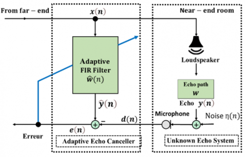
Within the framework of AEC, depicted in Figure 1, the microphone signal at time instant $n$ is given by:
$d(n)=y(n)+\eta(n)$ (1)
where, $\eta(\mathrm{n})$ indicates the presence of additive background noise with unknown power $\sigma_\eta^2$, and the acoustic echo signal $y(n)$ is generated as follows:
$y(n)=x^T(n) w$ (2)
where, the input signal vector $\boldsymbol{x}(n)=[x(n) x(n-$ 1) $\ldots x(n-M+1)]^T$ contains the most recent $M$ samples of the far-end signal, we assumed that this input signal is uncorrelated of the system noise $\eta(\mathrm{n})$ and $\boldsymbol{w}= \left[\begin{array}{llll}w_0 & w_1 & \ldots & w_{M-1}\end{array}\right]^T$ is a real acoustic impulse response, where $T$ denotes the matrix transposition. The estimated echo is obtained by:
$\hat{y}(n)=\widehat{w}^T(n-1) x(n)$ (3)
where, $\widehat{w}^T(n)=\left[\widehat{w}_0(n) \widehat{w}_1(n) \ldots \widehat{w}_{M-1}(n)\right]^T$ represents the estimation of the finite impulse response (FIR) and the error $e(n)$ of the AEC system expressed as:
$e(n)=d(n)-\hat{y}(n)$ (4)
Figure 1. The foundational architecture of AEC system
2.1 The NLMS algorithm
The NLMS algorithm is an improved version of the LMS algorithm that makes it easier to choose the adaptation step size for input signals such as speech. Therefore, we normalize the adaptation step of the LMS algorithm by a quantity depending on the power of the input signal [2]. The recursive update formula for the NLMS algorithm is given by [2]:
$\widehat{\boldsymbol{w}}(n)=\widehat{\boldsymbol{w}}(n-1)+\mu_{N L M S} \frac{\boldsymbol{x}(n) \boldsymbol{e}(n)}{\boldsymbol{x}^T(n) \boldsymbol{x}(n)+C_{N L M S}}$ (5)
where, $0<\mu_{N L M S}<2$ is referred to as the adaptation step and $C_{\text {NLMS}}$ is a regularization constant used to prevent division by values near zero, which can occur during periods of very low input signal energy. To achieve a total complexity approximately of $2 M$ operations for the NLMS, the term $\boldsymbol{x}^T(n) \boldsymbol{x}(n)$ of Eq. (5) can be expressed as a function of $P_x(n)$ and estimated recursively using the following expression:
$P_x(n)=\lambda P_x(n-1)+(1-\lambda) M x^2(n)$ (6)
where, $\lambda$ is a fixed forgetting factor.
2.2 The RLS algorithm
The RLS algorithm offers a more advanced and robust approach compared to the LMS and NLMS algorithms. Its primary objective is to iteratively minimize the least squares cost function of the error signal. By applying the matrix inversion lemma, the RLS algorithm significantly reduces computational complexity. This makes the RLS algorithm highly effective in scenarios demanding rapid convergence, particularly when dealing with correlated input signals. The mathematical formulation of the RLS algorithm [1] is given by the following set of equations:
$e(n)=d(n)-\widehat{\boldsymbol{w}}^T(n-1) \boldsymbol{x}(n)$ (7)
$\mathbf{K}(\mathrm{n})=\frac{\boldsymbol{R}^{-\mathbf{1}}(n-1) \boldsymbol{x}(n)}{\lambda_{R L S}+\boldsymbol{x}^T(n) \boldsymbol{R}^{-\mathbf{1}}(n-1) \boldsymbol{x}(n)}$ (8)
$\begin{array}{r}\boldsymbol{R}^{-\mathbf{1}}(n)=\frac{1}{\lambda_{R L S}}\left[\boldsymbol{R}^{-\mathbf{1}}(n-1)\right. \left.-\mathbf{K}(\mathrm{n}) \boldsymbol{x}^T(n) \boldsymbol{R}^{-\mathbf{1}}(n-1)\right]\end{array}$ (9)
$\widehat{\boldsymbol{w}}(n-1)=\widehat{\boldsymbol{w}}(n-1)+\mathbf{K}(\mathrm{n}) e(n)$ (10)
where, $K(n)$ is the Kalman gain vector and $R^{-1}(n)$ is an estimate inverse of the short-term correlation matrix defined by:
$\mathbf{R}(n)=\sum_{i=0}^n \lambda_{R L S}^{n-i} \boldsymbol{x}(i) \boldsymbol{x}^T(i)$ (11)
where, $\lambda_{R L S}$ is the exponential forgetting factor ( $0<\lambda_{R L S} \leq$ 1).
2.3 The fast NLMS algorithm
The FNLMS algorithm [6], inspired by the Fast Transversal Filter (FTF) technique [17, 18], provides a more efficient alternative to the Fast RLS algorithm by incorporating a decorrelation strategy for the input signal [19]. This algorithm is particularly valued for its rapid convergence and low computational complexity. A key advantage of the FNLMS algorithm is its ability to function without forward and backward predictors, which are essential in the FTF algorithm for computing the Kalman adaptation gain. By eliminating these predictors, the FNLMS algorithm effectively resolves the stability issues associated with the FTF approach, enhancing numerical robustness and reducing computational complexity. This results in an algorithm that not only surpasses the standard NLMS in performance but also achieves faster convergence and superior tracking capabilities. The adaptation gain for the FNLMS algorithm is given by Benallal and Arezki [6]:
$\boldsymbol{G}(n)=\gamma(n) \tilde{\mathbf{c}}(n)$ (12)
where, the dual Kalman gain is indicated by $\tilde{\mathbf{c}}(n)$ and the likelihood variable is represented by $\gamma(n)$. This approach leverages only a simple error prediction of the input signal $\boldsymbol{x}(n)$, eliminating the need for both forward and backward predictors. The update formula for the dual Kalman gain is given as:
$\left[\begin{array}{l}\tilde{\mathbf{c}}(n) \\ c(n)\end{array}\right]=\left[\begin{array}{c}-\frac{e_p(n)}{\lambda_{F N L M S} \alpha(n-1)+c_0} \\ \tilde{\boldsymbol{c}}(n-1)\end{array}\right]$ (13)
where, $c(n)$ is a scalar component, $e_p(n)$ represents the firstorder error in prediction, $\alpha(n)$ is the prediction error variance, and $c_0$ is a small positive constant used to avoid division by zero, and $\lambda_{F N L M S}$ is the exponential forgetting factor $0<\lambda_{F N L M S} \leq 1$. The prediction error is computed as follows:
$e_p(n)=x(n)-a(n) x(n-1)$ (14)
where, $a(n)$ represents the prediction parameter, which is estimated according to the following expression:
$a(n)=\frac{r_a(n)}{r_b(n)+c_a}$ (15)
where, $r_a(n)$ indicates an estimate of the first-lag correlation function of $x(n)$, while $r_b(n)$ serves as an estimate of the power of the input signal. These estimates can be derived using a recursive estimator, outlined as follows:
$r_a(n)=\lambda_a r_a(n-1)+x(n) x(n-1)$ (16)
$r_b(n)=\lambda_a r_b(n-1)+x^2(n)$ (17)
where, $\lambda_a$ is a fixed forgetting factor and $c_a$ is a small positive regularization constant. The variance of the prediction error is now evaluated using the following expression:
$\alpha(n)=\lambda_{F N L M S} \alpha(n-1)+e_p^2(n)$ (18)
The likelihood variable $\gamma(n)$ can be recursively expressed as:
$\gamma(n)=\frac{\gamma(n-1)}{1+\gamma(n-1) \delta(n)}$ (19)
where,
$\delta(n)=c(n) x(n-M)+\frac{x(n) e_p(n)}{\lambda_{\text {FNLMS }} \alpha(n-1)+c_0}$ (20)
The formula below represents the tap-update equation for the FNLMS algorithm [6]:
$\widehat{\boldsymbol{w}}(n)=\widehat{\boldsymbol{w}}(n-1)-\mu_{\text {ENLMS }} e(n) \gamma(n) \tilde{\boldsymbol{c}}(n)$ (21)
where, $\mu_{F N L M S}$ is a fixed step-size.
3.1 The practical VFF-RLS algorithm
The practical VFF-RLS algorithm, presented in reference [13] is designed to address system identification problems. As shown in references [8, 13], the choice of the forgetting factor $\lambda$ significantly impacts algorithm performance. A value of $\lambda$ close to 1 negatively influences the algorithm's tracking capability, while a lower λ value enhances tracking but can lead to increased misalignment and steady-state MSE in stationary environments.
The VFF employed in this algorithm is expressed as follows:
$\lambda(n)=\left\{\begin{array}{cc}\lambda_{\max } & \text { if } \zeta(n) \leq \varepsilon \\ \min \left[\frac{\sigma_q(n) \sigma_\eta(n)}{\left|\epsilon+\sigma_e(n)-\sigma_\eta(n)\right|}, \lambda_{\max }\right] & \text { if } \zeta(n)>\varepsilon\end{array}\right.$ (22)
where, $\epsilon$ is a small constant to prevent division by zero, $\lambda_{\text {max}}$ represents the maximum value of the forgetting factor and $\varepsilon$ is a small positive constant. The variable $\zeta(n)$ is called the convergence parameter.
Considering that [8, 13]:
$q(n)=x^T(n) R^{-1}(n-1) \times(n)$ (23)
where, E $\left\{q^2(n)\right\}=\sigma_q^2$, the power estimates are computed using an exponential window:
$\sigma_q^2(n)=\alpha \sigma_q^2(n-1)+(1-\alpha) q^2(n)$ (24)
where, $\alpha$ is a weighting factor, with $\alpha=1-1 /(K M)$ and $K>1$.
In this algorithm, the authors offer a more accurate and practical method to estimate system noise $\eta(\mathrm{n})$, this solution is highly precise, as system noise is typically stationary in practice, and it is calculated in reference [13] through the following steps:
The signal-to-noise ratio (SNR) is described as:
$S N R=\frac{\sigma_y^2}{\sigma_\eta^2}$ (25)
where, E $\left\{y^2(n)\right\}=\sigma_y^2$ is the variance of $y(n)$, in the context of adaptive filtering, we may additionally consider the estimated SNR as [13, 20]:
$S N R_f=\frac{\sigma_{\hat{y}}^2}{\sigma_e^2}$ (26)
where, $\sigma_{\hat{y}}^2=E\left\{\hat{y}^2(n)\right\}$. As the adaptive filter approaches its steady-state condition, it is expected that [13]:
$\hat{y}(n) \approx y(n)$ (27)
And, consequently:
$e(n) \approx \eta(n)$ (28)
Therefore, in this case:
$S N R_f \approx S N R$ (29)
Since $y(n)$ and $\eta(n)$ are uncorrelated, allowing Eq. (1) to be reformulated in terms of variances as:
$\sigma_d^2(n)=\sigma_y^2(n)+\sigma_\eta^2(n)$ (30)
By developing Eq. (29) and considering Eq. (30), the estimate of the system noise power in steady-state can be calculated as follows [13]:
$\sigma_\eta^2(n)=\frac{\sigma_d^2(n) \sigma_e^2(n)}{\sigma_e^2(n)+\sigma_{\hat{y}}^2(n)}$ (31)
where, the power estimates in Eq. (31) are calculated recursively using:
$\sigma_d^2(n)=\alpha \sigma_d^2(n-1)+(1-\alpha) d^2(n)$ (32)
$\sigma_e^2(n)=\alpha \sigma_e^2(n-1)+(1-\alpha) e^2(n)$ (33)
$\sigma_{\hat{y}}^2(n)=\alpha \sigma_{\hat{y}}^2(n-1)+(1-\alpha) \hat{y}^2(n)$ (34)
In terms of energy, Eq. (28) becomes:
$\sigma_e^2(n) \approx \sigma_\eta^2(n)$ (35)
Thus, substituting Eq. (31) into Eq. (35) yields:
$\sigma_d^2(n) \approx \sigma_{\hat{y}}^2(n)+\sigma_e^2(n)$ (36)
From Eq. (36). the convergence parameter $\zeta(n)$ is defined as follows [13]:
$\zeta(n)=\left|\sigma_d^2(n)-\sigma_{\hat{y}}^2(n)-\sigma_e^2(n)\right|$ (37)
|
Algorithm 1: PVFF-RLS Algorithm |
|
Initialization $\begin{aligned} & \widehat{\boldsymbol{w}}(0)=0, \boldsymbol{R}^{-1}(0)=\rho \mathbf{I}_M, \sigma_d^2(0)=0.1, \sigma_q^2(0)=0.1, \sigma_{\hat{y}}^2(0)= \\ & 0.1, \sigma_e^2(0)=0.1\end{aligned}$ |
|
$\mathbf{n}=1,2, \ldots$ (iterations) $q(n)=\boldsymbol{x}^T(n) \boldsymbol{R}^{-1}(n-1) \boldsymbol{x}(n)$ $\sigma_q^2(n)=\alpha \sigma_q^2(n-1)+(1-\alpha) q^2(n)$ $\begin{aligned} & \sigma_d^2(n)=\alpha \sigma_d^2(n-1)+(1-\alpha) d^2(n) \\ & \sigma_{\hat{y}}^2(n)=\alpha \sigma_{\hat{y}}^2(n-1)+(1-\alpha) \hat{y}^2(n) \\ & \sigma_e^2(n)=\alpha \sigma_e^2(n-1)+(1-\alpha) e^2(n)\end{aligned}$ $\begin{aligned} & \sigma_\eta^2(n)=\frac{\sigma_d^2(n) \sigma_e^2(n)}{\sigma_e^2(n)+\sigma_{\hat{y}}^2(n)} \\ & \zeta(n)=\left|\sigma_d^2(n)-\sigma_{\hat{y}}^2(n)-\sigma_e^2(n)\right|\end{aligned}$ $\lambda(n)=\left\{\begin{array}{cc}\lambda_{\max } & \text { if } \zeta(n) \leq \varepsilon \\ \min \left[\frac{\sigma_q(n) \sigma_\eta(n)}{\left|\epsilon+\sigma_e(n)-\sigma_\eta(n)\right|}, \lambda_{\max }\right] & \text { if } \zeta(n)>\varepsilon\end{array}\right.$ $\boldsymbol{K}(n)=\frac{\boldsymbol{x}(n) \boldsymbol{R}^{-\mathbf{1}}(n-1)}{\lambda(n)+q(n)}$ $\boldsymbol{R}^{-1}(n)=\frac{1}{\lambda(n)}\left[\boldsymbol{R}^{-1}(n-1)-\boldsymbol{K}(n) \boldsymbol{x}^T(n) \boldsymbol{R}^{-1}(n-1)\right]$ Filtering Error $e(n)=d(n)-\widehat{\boldsymbol{w}}^T(n-1) \boldsymbol{x}(n)$ Filter update $\widehat{\boldsymbol{w}}(n)=\widehat{\boldsymbol{w}}(n-1)+\boldsymbol{K}(n) e(n)$ |
This parameter $\zeta(n)$ distinguishes between steady-state and tracking phases, where when the unknown system changes (in tracking scenario), the error become large, so that $\zeta(n)>\varepsilon$, during the steady-state phase, we have $\zeta(n) \leq \varepsilon$ [13]. Algorithm 1 provides the practical VFF-RLS algorithm (PVFF-RLS). A significant drawback of this algorithm is its high computational complexity, which limits its practicality in real-world applications such as AEC. In addition, previous VFF-RLS algorithms have always been tested under abrupt system changes, which are not representative of practical scenarios. As a consequence, subsequent simulation results reveal difficulties in tracking the temporal variations of the unknown system in a non-stationary environment, due to forgetting factor values close to 1. To address these challenges, the next section presents a novel approach with several advantages. It demonstrates superior tracking capabilities compared to the NLMS, RLS, FNLMS, and PVFF-RLS algorithms. Additionally, it outperforms the FNLMS algorithm in terms of convergence speed, final MSE, and misalignment. Significantly, this improved approach achieves these performance enhancements while maintaining lower computational complexity compared to the PVFF-RLS algorithm.
3.2 The proposed VFF FNLMS algorithm
The proposed NVFF design is inspired by the Variable Step-Size (VSS) principle, and has been carefully developed to achieve the key objective of dynamically adjusting the forgetting factor to balance convergence stability and tracking capability. Unlike VSS, where the step size is increased in non-stationary conditions, our NVFF inverts this principle: the forgetting factor is kept close to 1 in stationary conditions to minimize misalignment and set slightly below 1 in non-stationary conditions to enable rapid adaptation. This formulation ensures an optimal trade-off between convergence and tracking and is theoretically supported by a mathematical analysis of $\lambda$ behavior across three scenarios: pre-convergence, stationary, and non-stationary. Moreover, unlike existing VFF-RLS algorithms, which not only suffer from high computational complexity but are also typically tested under abrupt system changes that do not reflect realistic conditions, our evaluation on both artificial and real time-varying systems demonstrated that such approaches struggle to maintain effective tracking. These limitations motivated the development of the NV16FF-FNLMS, which combines low complexity with robust performance in practical scenarios.
This approach is founded upon a fundamental criterion related to the variation in the forgetting factor, defined by the energy ratio between error power and noise power this fundamental criterion justified by the fact that the error significantly varies between stationary and non-stationary systems: it is small in stationary conditions and large in non-stationary conditions. Therefore, based on the error value, the forgetting factor can be dynamically adjusted to optimize the algorithm’s performance. Formally, this criterion is expressed as:
$\lambda(n)=1-\varphi\left|\frac{\sigma_e^2(n)-\sigma_\eta^2(n)}{\sigma_e^2(n)}\right|$ (38)
where, $0<\varphi<1$, serves as a constant that regulates the VFF. In the proposed algorithm, the error signal is estimated using an exponential windowas follow:
$\sigma_e^2(n)=\beta \sigma_e^2(n-1)+(1-\beta) e^2(n)$ (39)
where, $\beta$ is a weighting forgetting factor.
Using the method described in reference [21], the system noise variance can be estimated from $e(n)$ as follows:
$\sigma_n(n)=\sigma_{|e|}(n)$ (40)
where,
$\sigma_{|e|}(n)=\beta \sigma_{|e|}(n-1)+(1-\beta)|e(n)|$ (41)
3.2.1 Derivation of the variable forgetting factor NVFF
In this subsection, we derive the expression for the forgetting factor $\lambda(n)$ in three distinct scenarios preconvergence, stationary, and non-stationary to illustrate how $\lambda(n)$ adapts dynamically in each case.
At startup, before the filter converges, during the learning phase, we can approximately write:
$\hat{y}(n) \approx 0$ (42)
Substituting Eq. (42) in Eq. (4), we obtain:
$e(n) \approx d(n)$ (43)
Consequently, in terms of energy, Eq. (43) will be:
$\sigma_e^2(n) \approx \sigma_d^2(n)$ (44)
By using Eq. (30) and Eq. (44) in Eq. (38), the $\lambda(n)$ can be expressed as follows:
$\lambda(n)=1-\varphi\left|\frac{\sigma_y^2(n)}{\sigma_y^2(n)+\sigma_\eta^2(n)}\right|$ (45)
$\lambda(n)=1-\varphi\left|\frac{1}{1+S N R^{-1}}\right|<1$ (46)
From Eq. (46), it is evident that $\lambda(n)$ remains strictly less than 1, indicating that $\lambda(n)$ starts at a value smaller than one during the initial phase, whatever of the SNR value.
In this case, the forgetting factor by definition should be set very close to 1. This maximizes convergence speed, minimizes the final mean-square error (MSE), and reduces misalignment. Aassuming the filter has sufficiently converged to its true value for Eq. (35) to be satisfied, the VFF in the proposed approach can be expressed as:
$\lambda(n)=1-\varphi\left|\frac{\sigma_\eta^2(n)-\sigma_\eta^2(n)}{\sigma_e^2(n)}\right| \approx 1$ (47)
The forgetting factor reaches its maximum value in the stationary case. However, if the echo system changes over time, disturbances may affect the echo signal, represented as:
$y(n)+y_{n s}(n)$ (48)
where, $y_{n s}(n)$ is a disturbance resulting from temporal variations of the unknown system, and $y(n)$ stays near to $\hat{y}(n)$. Consequently, the desired signal $d(n)$ in Eq. (1) becomes:
$d(n)=y(n)+y_{n s}(n)+\eta(\mathrm{n})$ (49)
Assuming $y(n), y_{n s}(n)$ and $\eta(\mathrm{n})$ are independent quantities, the energy of $d(n)$ can be approximated as:
$\sigma_d^2(n)=\sigma_y^2(n)+\sigma_{y_{n s}}^2(n)+\sigma_\eta^2(n)$ (50)
Furthermore, by equating Eq. (36) and Eq. (50) and applying the assumption $\sigma_y^2(n) \approx \sigma_{\hat{y}}^2(n)$, the error power can be represented through an alternative expression:
$\sigma_e^2(n) \approx \sigma_{y_{n s}}^2(n)+\sigma_\eta^2(n)$ (51)
As a result, substituting Eq. (51) into Eq. (38) yields:
$\lambda(n) \approx 1-\varphi\left|\frac{\sigma_{y_{n s}}^2(n)}{\sigma_{y_{n s}}^2(n)+\sigma_n^2(n)}\right|$ (52)
In Eq. (52), it is important to observe that the term $\left|\frac{\sigma_{y_{n s}}^2(n)}{\sigma_{y_{n s}}^2(n)+\sigma_\eta^2(n)}\right|$ always lies between 0 and 1, as the denominator is greater than the numerator, ensuring:
$0<\left|\frac{\sigma_{y_{n s}}^2(n)}{\sigma_{y_{n s}}^2(n)+\sigma_\eta^2(n)}\right|<1$ (53)
As a result, we have:
$0<1-\varphi\left|\frac{\sigma_{y_{n s}}^2(n)}{\sigma_{y_{n s}}^2(n)+\sigma_\eta^2(n)}\right|<1$ (54)
Thus, in the non-stationary case we conclude that:
$0<\lambda(n)<1$ (55)
Finally, the VFF expression for the proposed NVFF-FNLMS is given by:
$\lambda(n)=\left\{\begin{array}{cc}\lambda_{\max } & \text { if } \zeta(n) \leq \varepsilon \\ 1-\varphi\left|\frac{\sigma_e^2(n)-\sigma_\eta^2(n)}{\sigma_e^2(n)+\delta_0}\right| & \text { if } \zeta(n)>\varepsilon\end{array}\right.$ (56)
where, $\delta_0$ small constant is added to avoid division by zero. The recursive estimators of $\sigma_d^2(n)$ and $\sigma_{\hat{y}}^2(n)$ are estimated as follows:
$\sigma_d^2(n)=\beta \sigma_d^2(n-1)+(1-\beta) d^2(n)$ (57)
$\sigma_{\hat{y}}^2(n)=\beta \sigma_{\hat{y}}^2(n-1)+(1-\beta) \hat{y}^2(n)$ (58)
In this NVFF-FNLMS algorithm, the choice of the parameter $\varphi$ is critical to ensure effective performance, as it governs the behavior of the forgetting factor $\lambda(n)$, which must always remain strictly less than 1 . Theoretically, $\varphi$ must be smaller than 1, a condition derived from the analysis of Eq. (46) under the assumption that the SNR is always positive. After mathematical manipulation, Eq. (46) yields the following condition:
$0<\varphi<1+\mathrm{SNR}^{-1}$ (59)
Since $\mathrm{SNR}^{-1}$ is typically much smaller than unity, for example, at $\mathrm{SNR}=50 \mathrm{~dB}$ we have $\mathrm{SNR}^{-1}=0.00001$, it can be approximated that $1+\mathrm{SNR}^{-1} \approx 1$. Consequently, the simplified condition is obtained as follows:
$\varphi<1$ (60)
Furthermore, for noise estimation method $\sigma_\eta(n)=\sigma_{|e|}(n)$ in (40) it is important to note that this approximation is a simplified assumption. In the non-stationary case, the error signal can be expressed as $e(n)=\eta(n)+y_{n s}(n)$. Consequently, the error power is approximated by $\sigma_e^2(n) \approx \sigma_{y_{n s}}^2(n)+\sigma_\eta^2(n)$, This decomposition shows that the error is not purely due to noise, but also contains a component related to system variations. From a noise estimation viewpoint, this assumption introduces a drawback, since part of the error variance is wrongly interpreted as noise, leading to an overestimation of $\sigma_\eta^2(n)$. However, the presence of $y_{n s}(n)$ in the error signal can also be regarded as beneficial for tracking, because it implicitly conveys information about system variations and enables the VFF to adapt more effectively in non-stationary environments. Therefore, while this estimation method is reliable in stationary conditions, its limitation in non-stationary cases should be acknowledged, as it simultaneously degrades the accuracy of noise estimation but enhances the tracking capability of the algorithm.
Finally, the theoretical analysis reveals that the proposed NVFF aligns with the general principle of a VFF. When the real system exhibits stationary behavior, the proposed NVFF approaches a value of one, enabling the algorithm to achieve a lower steady-state error. In contrast, under non-stationary conditions, the denominator in Eq. (52) increases, resulting in a decrease in the forgetting factor $\lambda(n)$ to lower values, which enhances the algorithm’s ability to track time variations of the system.
3.2.2 Stability analysis of the proposed NVFF-FNLMS
To establish the stability condition of the newly proposed NVFF-FNLMS algorithm, which is a variant of the FNLMS algorithm incorporating a VFF technique, we refer to the stability and convergence condition of the adaptation step-size $\mu_{F N L M S}$ derived in reference [6]. This condition is itself related to the adaptation step-size $\mu_{N L M S}$ of the classical NLMS algorithm, obtained using approximate mean-square analysis as described by Slock [22]. The analysis focuses on how the FNLMS algorithm influences the adaptation gain compared to the NLMS algorithm. For this purpose, we assume that the input signal is a white Gaussian stationary process. Under this assumption, we can approximate $e_p(n) \approx x(n)$, and the variance of the prediction error $\alpha(n)$ for the proposed algorithm is evaluated as follows:
$\alpha(n)=\lambda(n) \alpha(n-1)+x^2(n)$ (61)
The Eq. (61) can be expanded iteratively as:
$\alpha(n)=\lambda(n)\left[\lambda(n-1) \alpha(n-2)+x^2(n-1)\right]+x^2(n)$ (62)
$\alpha(n)=\lambda(n) \lambda(n-1) \alpha(n-2)+\lambda(n) x^2(n-1)+x^2(n)$ (63)
$\begin{gathered}\alpha(n)=\alpha(0) \prod_{i=1}^n \lambda(i) +\sum_{k=0}^{n-1}\left[x^2(n-k) \prod_{j=0}^{k-1} \lambda(n-j)\right]\end{gathered}$ (64)
where, we adopt the convention that the empty product is equal to 1. If we now consider the expected value under the assumption that $x(n)$ is a stationary white Gaussian process with variance $\sigma_x^2$, we obtain:
$\begin{aligned} & E\{\alpha(n)\}=E\{\alpha(0)\} \prod_{i=1}^n E\{\lambda(i)\} & +\sigma_x^2 \sum_{k=0}^{n-1} \prod_{j=0}^{k-1} E\{\lambda(n-j)\}\end{aligned}$ (65)
Based on the stationary case, in the steady state we observe that $\lambda(n)$ is almost constant and close to 1. Therefore, $\lambda(n)$ tends toward a stationary value, denoted as $\lambda_{\text {sta}}$ (the stationarycase) very close to 1 (slightly less than unity for analysis purposes). Under this assumption, the expression simplifies to:
$\begin{gathered}E\{\alpha(n)\}=\alpha(0) \lambda_{\mathrm{sta}}{ }^n+\sigma_x^2 \sum_{k=0}^{n-1} \lambda_{\mathrm{sta}}{ }^k \\ =\alpha(0) \lambda_{\mathrm{sta}}{ }^n+\sigma_x^2 \frac{1-\lambda_{\mathrm{sta}}}{1-\lambda_{\mathrm{sta}}}\end{gathered}$ (66)
Thus, for $n \rightarrow \infty$, the mean variance of the prediction error signal converges to:
$\alpha(n)=\frac{\sigma_x^2}{1-\lambda_{\mathrm{sta}}}$ (67)
Now we also adjust the other equations of $\tilde{\boldsymbol{c}}(n)$ and $\gamma(n)$ by their asymptotic values:
$\tilde{\mathbf{c}}(n)=\frac{\boldsymbol{x}(n)}{\frac{\lambda_{\text {sta }}}{1-\lambda_{\text {sta }}} \sigma_x^2+c_0}$ (68)
$\gamma(n)=\frac{1}{1-\tilde{\mathbf{c}}(n) \boldsymbol{x}(n)} \approx \frac{1}{1+\frac{M \sigma_x^2}{\frac{\lambda_{\mathrm{sta}} \sigma_x^2}{1-\lambda_{\mathrm{sta}}}+c_0}}$ (69)
The adaptation gain of the NLMS algorithm, under the stability condition $0<\mu_{N L M S}<2$, is approximately given by [6, 17]:
$\tilde{\mathbf{c}}_{N L M S}(n) \approx-\frac{\bar{\mu}_{N L M S}}{M \sigma_x^2} \boldsymbol{x}(n)$ (70)
By applying the approximations in Eqs. (67)-(69), the adaptation gain of the proposed NVFF-FNLMS algorithm can be expressed as follows:
$\begin{gathered}\tilde{\mathbf{c}}(n) \approx-\frac{\mu_{N L M S}}{M \sigma_x^2\left(1+\frac{\lambda_{\mathrm{sta}}}{M\left(1-\lambda_{\mathrm{sta}}\right)}+\frac{c_0}{M \sigma_x^2}\right)} \boldsymbol{x}(n) \\ \approx-\frac{\mu_{N L M S}}{M \sigma_x^2\left(1+\frac{\lambda_{\mathrm{sta}}}{M\left(1-\lambda_{\mathrm{sta}}\right)}+\frac{c_0}{M \sigma_x^2}\right)} \boldsymbol{x}(n)\end{gathered}$ (71)
Finally, by comparing Eqs. (70) and (71), the condition stabiliti of the proposed algorithm can be stated as:
$0<\mu_{\mathrm{NVF}}=\frac{\mu_{N L M S}}{1+\frac{\lambda_{\text {stat }}}{\left(1-\lambda_{\text {stat }}\right) M}+\frac{c_0}{M \sigma_x^2}}<2$ (72)
Based on the stability condition of the NVFF formulation, we find that this inequality is always satisfied for $0<\mu_{N L M S}<2$. Moreover, from the derivation of $\lambda(n)$ in the pre-convergence, stationary, and non-stationary cases, we observe that $0< \lambda(n)<1$. Therefore, we conclude that the proposed algorithm is stable even when the forgetting factor varies dynamically.
Algorithm 2 gives an overview of the proposed algorithm.
|
Algorithm 2: NVFF-FNLMS Algorithm |
|
Initialization: $\begin{aligned} & \widehat{\boldsymbol{w}}(0)=0, c_a=c_0=0.1, r_a(0)=0, \alpha(0)=r_b(0)=5, \gamma(0)= \\ & 1, \sigma_{|e|}(0)=0.1, \sigma_d^2(0)=0.1, \sigma_{\hat{y}}^2(0)=0.1, \sigma_e^2(0)=0.1\end{aligned}$ |
|
For $\mathbf{n}=1,2, \ldots$ (iterations) Adaptation gain $\begin{aligned} & r_a(n)=\lambda_a r_a(n-1)+x(n) x(n-1) \\ & r_b(n)=\lambda_a r_b(n-1)+x^2(n) \\ & a(n)=\frac{r_a(n)}{r_b(n)+c_a} \\ & e_p(n)=x(n)-a(n) x(n-1) \\ & \sigma_d^2(n)=\beta \sigma_d^2(n-1)+(1-\beta) d^2(n) \\ & \sigma_{\hat{y}}^2(n)=\beta \sigma_{\hat{y}}^2(n-1)+(1-\beta) \hat{y}^2(n) \\ & \sigma_e^2(n)=\beta \sigma_e^2(n-1)+(1-\beta) e^2(n) \\ & \sigma_{|e|}(n)=\beta \sigma_{|e|}(n-1)+(1-\beta)|e(n)| \\ & \sigma_\eta(n)=\sigma_{|e|}(n)\end{aligned}$ $\begin{aligned} & \zeta(n)=\left|\sigma_d^2(n)-\sigma_{\hat{y}}^2(n)-\sigma_e^2(n)\right| \\ & \lambda(n)=\left\{\begin{aligned} \lambda_{\max } & \text { if } \zeta(n) \leq \varepsilon \\ 1-\varphi\left|\frac{\sigma_e^2(n)-\sigma_\eta^2(n)}{\sigma_e^2(n)+\delta_0}\right| & \text { if } \zeta(n)>\varepsilon\end{aligned}\right. \\ & \alpha(n)=\lambda(n) \alpha(n-1)+e_p^2(n) \\ & {\left[\begin{array}{l}\widetilde{\mathbf{c}}(n) \\ c(n)\end{array}\right]=\left[\begin{array}{c}-\frac{e_p(n)}{\lambda(n) \alpha(n-1)+c_0} \\ \widetilde{\boldsymbol{c}}(n-1)\end{array}\right]} \\ & \delta(n)=x(n-M) c(n)+\frac{x(n) e_p(n)}{\lambda(n) \alpha(n-1)+c_0} \\ & \gamma(n)=\frac{\gamma(n-1)}{\delta(n) \gamma(n-1)+1}\end{aligned}$ |
|
Filtering Error $e(n)=d(n)-\widehat{\boldsymbol{w}}^T(n-1) \boldsymbol{x}(n)$ Filter update $\widehat{\boldsymbol{w}}(n)=\widehat{\boldsymbol{w}}(n-1)-\mu_{N V F F} e(n) \gamma(n) \tilde{\boldsymbol{c}}(n)$ |
We compare the performance of the proposed NVFF-FNLMS algorithm with those of the NLMS, RLS, FNLMS, and PVFF-RLS algorithms in an AEC system simulation. Three different input signals were used in many simulation tests, along with stationary and non-stationary systems. The performance evaluation is based on two criteria. To begin, we will provide an overview of the features associated with the signals utilized in this study.
4.1 Description of simulation signals and systems
4.1.1 Presentation of stationary and non-stationary signals
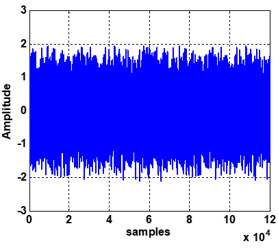
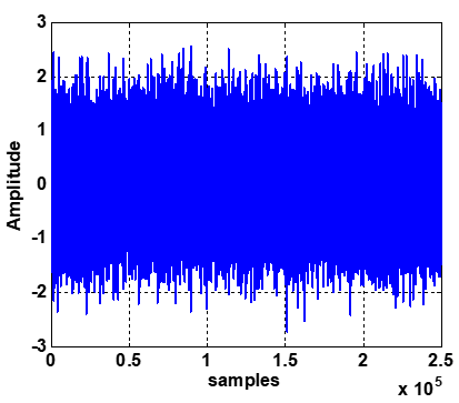
Throughout the simulations, we introduced three different types of input signals. Each of these signals was recorded at a 16kHz sampling rate and represented in 16-bit amplitude. The initial signal, referred to as the USASI signal (United States of America Standards Institute), is defined as a real, stationary, correlated noise. Its spectrum closely aligns with the average speech spectrum, exhibiting a spectral range of 32dB and a power of $\sigma_x^2=$ 0.32. Furthermore, this signal has a Gaussian probability distribution and is widely used in AEC applications [2, 3], as shown in Figure 2. During our simulation study, we also incorporated a second stationary signal, referred to as WGN- AR20, this signal is the result of the filtering of a stationary white Gaussian noise by an autoregressive model of order 20 derived from a speech sentence. It is highly correlated (more so than the USASI signal) and has a spectral range of around 42dB, with a mean power of $\sigma_x^2=$ 0.37, as shown in Figure 3.
Figure 2. USASI input signal
Figure 3. WGN-AR20 input signal
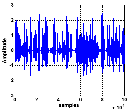
Figure 4. Speech input signal
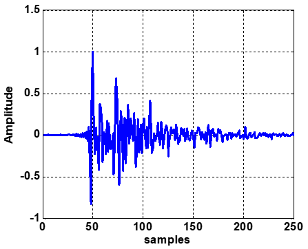
We assessed the algorithms in a real-time acoustic echo scenario utilizing a non-stationary real speech signal as the last input signal, as shown in Figure 4, this signal achieved by combining two sentences, one male and one female, each lasting 6.75 seconds. It has a spectral dynamic range of 46dB, with an estimated speech power of $\sigma_x^2=0.15$, and approximately follows the Laplace distribution in its probability characteristics. Filtering the input signal with a 256- and 512-point real car acoustic impulse response (see Figure 5) produces the acoustic echo signal. Finally, to generate the desired signal, a white Gaussian noise component is added to the echo signal with a given SNR. In Section 4.4.4, we examine the experimental scenario of non-stationary systems implemented in a real acoustic environment.
Figure 5. Car acoustic impulse response (M = 256)
4.1.2 Presentation of artificial non-stationary systems
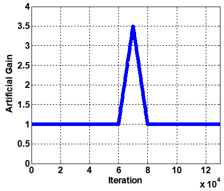
The acoustic channel is modified by multiplying the impulse response $\boldsymbol{w}(n)$ with a gain function for a finite duration, specifically from 60,000 to 80,000 iteration samples, with an amplitude varying linearly between 1 and 3.5 in an increasing then decreasing order, as shown in Figure 6. This is done to assess the ability of an adaptive algorithm to track changes in the unknown system as they occur.
Figure 6. Variation in gain for the tracking experiment
4.2 Description of performance criteria
To assess the effectiveness of adaptive algorithms in echo cancellation, various criteria have been established. In this paper, we utilize two specific criteria, namely:
4.2.1 Mean square error (MSE) criterion
This is the Criterion of the temporal evolution of the MSE in dB for the comparison between algorithms, determined by:
$\operatorname{MSE}_{d B}(n)=10 \log _{10}\left(<e^2(n)>\right)$ (73)
where, the symbol $<.>$ represent temporal averages over 256, 512 and 1024 samples.
4.2.2 Misalignment criterion
The Misalignment criterion serves as a robust metric for evaluating the effectiveness of adaptive algorithms. It quantifies the discrepancy among the coefficients of the actual impulse response and those of the estimated filter in dB, calculated as:
Misalignment $_{d B}(n)=10 \log _{10}\left[\frac{\|\boldsymbol{w}-\widehat{\boldsymbol{w}}(n)\|^2}{\|\boldsymbol{w}\|^2}\right]$ (74)
where, the symbol $\|$.$\|$ denotes the Euclidean norm $l_2$.
4.3 Presentation of the used parameters
In all AEC simulations conducted in this study, which involved comparing the performance of the proposed NVFFFNLMS algorithm with existing adaptive algorithms, it was crucial to appropriately set key parameters, considering the presence of additive noise. In the absence of noise, we set the adaptation step size to one to achieve the fastest possible convergence speed. However, in noisy environments, it is generally advisable to select value less than one [23, 24]. In our results we fixed $\mu_{N L M S}$ to 0.7, these chosen parameters are intended to yield similar steady-state MSE across all tested algorithms in the stationary scenario, the regularization constant is fixed as $C_{N L M S}=20 \sigma_x^2$ for NLMS algorithm. For the FNLMS algorithm, there are two distinct forgetting factors, the first, $\lambda_{F N L M S}$ for tracking system changes in the unknown system [6, 17] and was set to $\lambda_{F N L M S}=1-\frac{1}{3 M}$ to achieve good performance in terms of convergence speed and tracking ability. The second, $\lambda_{\mathrm{a}}$ for tracking the non-stationarity of the input signal [9], its value is $\lambda_{\mathrm{a}}=1-\frac{1}{3.5 M}$, the same value of $\lambda_{\mathrm{a}}$ was also fixed in the NVFF-FNLMS algorithm, the stepsize to FNLMS algorithm is $\mu_{F N L M S}=1$.and $\mu_{N V F F}=1$ for the proposed NVFF-FNLMS. Additional parameters used in both FNLMS and NVFF-FNLMS algorithms included: $c_a= c_0=0.1, r_a(0)=0, \alpha(0)=r_b(0)=5$ and $\gamma(0)=1$.
For the RLS algorithm, the forgetting factor was fixed to $\lambda_{R L S}=1-\frac{1}{3 M}$, the same value of $\lambda_{F N L M S}$ used for the FNLMS algorithm in all simulations in this paper. Regarding the PVFF-RLS algorithm, initial values were: $\sigma_d^2(0)= \sigma_q^2(0)=\sigma_{\hat{y}}^2(0)=\sigma_e^2(0)=0.1$, and we set the weighting factor $\alpha=1-1 /(K M)$ with $K=6$ [13, 25], and $\rho$ is a small positive constant of the order of $10^{-4}$.Additionally, $\lambda_{\max }$ was set to 1 for both the PVFF-RLS and the proposed NVFFFNLMS algorithms. The parameters $\epsilon$ and $\delta_0$, appearing in the denominators of Eq. (22) and Eq. (56), respectively, were fixed at $\epsilon=\delta_0=10^{-3}$.
For the parameter $\varphi$, any value strictly less than 1 can be chosen, as demonstrated theoretically. However, in practical applications such as (SI) or (AEC) applications, it is preferable to select a sufficiently robust value of $\varphi$ to cope with different scenarios (noise variations, tracking requirements, etc.). To this end, and after extensive testing, we fixed $\varphi=0.9$ for all simulations. Furthermore, we conducted experiments with several values of $\varphi$ to evaluate and compare their effect on the algorithm's performance.
For the weighting parameter $\beta$, values close to 1 (e.g., $0.9989,0.998$, or $0.99, \ldots$.) are widely adopted in the adaptive filtering literature to ensure smooth variance estimation while maintaining responsiveness to changes in noise levels. This is consistent with standard practices in recursive estimators [1, 2]. In this study, $\beta$ was chosen based on a window size of 909 samples, leading to $\beta=1-\frac{1}{909} \approx 0.9989$. The initial values for the NVFF-FNLMS were set as: $\sigma_{|e|}(0)=\sigma_d^2(0)= \sigma_{\hat{y}}^2(0)=0.1, \sigma_e^2(0)=0.1$. performance of the suggested NVFF-FNLMS algorithm. The impulse responses used in this article were relatively long ( 256 and 512 samples), and it is important to note that the parameters mentioned earlier remain consistent across all the experimental results presented in this section.
4.4 Comparison results
4.4.1 Case of a stationary input signal and system
The first step in our study is to compare the proposed NVFF-FNLMS algorithm with the conventional NLMS and FNLMS algorithms. The results, presented in Figures 7 and 8, were obtained using USASI noise with filter length $M=256$ and SNR values of 5dB and 50dB. These experiments focus on the AEC application, where the algorithm performance is evaluated in terms of the MSE.
Figure 7. Comparison of MSE evolution for USASI noise, $M=256, \mathrm{SNR}=5 \mathrm{~dB}, \varepsilon=0.01$
Figure 8. Comparison of MSE evolution for USASI noise, $M=256, \mathrm{SNR}=50 \mathrm{~dB}, \varepsilon=0.01$
The evaluation based on the MSE clearly demonstrates that the proposed NVFF-FNLMS algorithm outperforms both NLMS and FNLMS. It achieves faster convergence and, importantly, improves the steady-state MSE compared to the conventional algorithms. The results show that the algorithm remains effective in echo attenuation across different SNR conditions, with significant performance differences observed between low SNR (5dB) and high SNR (50dB) scenarios.
In the second set of experiments of this case, presented in Figures 9 and 10, the algorithm was evaluated for System Identification (SI) application using the same SNR values of 5dB and 50dB. In this application, performance was assessed using the Misalignment criterion, which measures the deviation between the estimated and actual system outputs, providing an accurate assessment of identification accuracy. The results show that the NVFF-FNLMS algorithm maintains superior lower misalignment compared to NLMS and FNLMS, confirming its robustness and effectiveness for both AEC and SI applications under varying noise conditions.
Figure 9. Comparison of misalignment evolution for USASI noise, $M=256, \mathrm{SNR}=5 \mathrm{~dB}, \varepsilon=0.01$
Figure 10. Comparison of misalignment evolution for USASI noise, $M=256, \mathrm{SNR}=50 \mathrm{~dB}, \varepsilon=0.01$
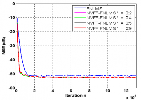
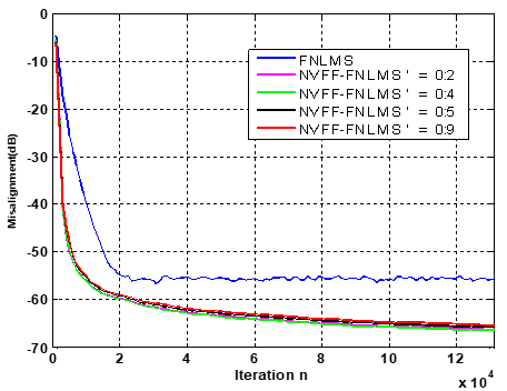
In this paragraph, we investigate the impact of the parameter $\varphi$ on the performance of the proposed NVFF-FNLMS algorithm, as illustrated in Figures 11 and 12. The algorithm was tested with several values of $\varphi$ in order to analyze and compare their influence on convergence speed misalignement and steady-state performance, evaluated using the MSE and MSD criterion with SNR $=50 \mathrm{~dB}$ and filter length $M=256$.
Figure 11. Analysis of MSE for the NVFF-FNLMS with various $\varphi$ values using USASI noise, $\mathrm{M}=256$, and $\mathrm{SNR}=50 \mathrm{~dB}$
Figure 12. Analysis of misalignment for the NVFF-FNLMS with various $\varphi$ values using USASI noise, $\mathrm{M}=256$, and $\mathrm{SNR}=50 \mathrm{~dB}$
These results confirm that the algorithm remains stable and effective across a wide range of $\varphi$ values, thereby validating the robustness of the parameter choice.
4.4.2 Case of a non-stationary system and stationary input signal
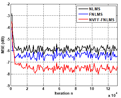
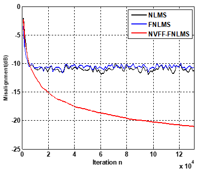
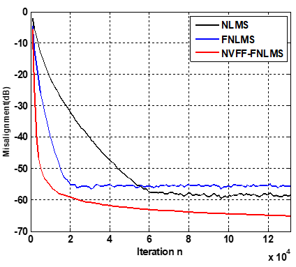
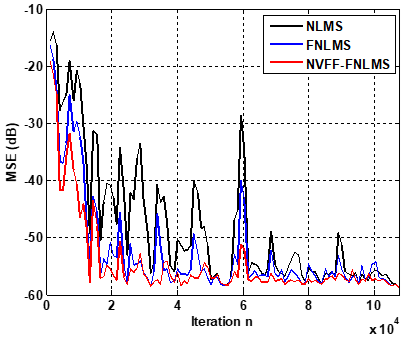
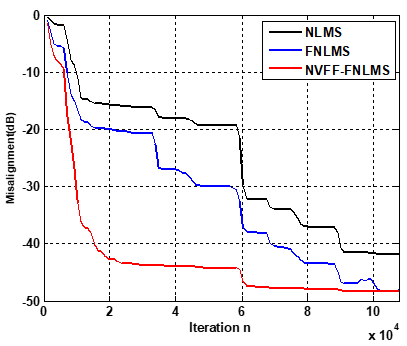
For this scenario, we started by evaluating the proposed algorithm and comparing its performance with classical NLMS and FNLMS algorithms over extended trials. These evaluations were carried out with an artificial time-varying system, as shown in Figure 6. The results depicted in Figures 13 and 14 underscore the superior tracking performance of the proposed algorithm, which is attained by utilizing the WGN-AR20 signal convolved with an artificially time-varying impulse response.
Figure 13. Comparison of misalignment evolution for WGN-AR20 input,$M=512, \mathrm{SNR}=50 \mathrm{~dB}, \varepsilon=0.0001$
Figure 14. Comparison of MSE evolution for WGN-AR20 input, $M=512, \mathrm{SNR}=50 \mathrm{~dB}, \varepsilon=0.0001$
In addition, Table 1 provides a quantitative comparison of the convergence times for the NLMS, FNLMS, and the proposed NVFF-FNLMS algorithms. The analysis is based on the average number of iterations required to reach the steady-state MSE, referred to as the convergence time constant. This was defined as the point where the MSE variation remains within ±1dB over 10 consecutive blocks. This approach enables a robust and adaptive detection of convergence, avoiding the use of an arbitrary threshold such as –30dB, while allowing for fair comparison across all evaluated algorithms. The evaluation was performed using two input signals (USASI and WGN-AR20) and two filter lengths (M=256 and M=512).
Table 1. Convergence time analysis, comparing NLMS, FNLMS and NVFF-FNLMS
|
Convergence Rate [Iteration] |
||||
|
|
USASI |
WGN-AR20 |
||
|
Algorithms |
M=256 |
M=512 |
M=256 |
M=512 |
|
NLMS |
37888 |
74752 |
87654 |
137564 |
|
FNLMS |
12288 |
24576 |
69632 |
110592 |
|
NVFF-FNLMS |
9216 |
18331 |
22528 |
29696 |
The results in Table 1 demonstrate that the proposed NVFF-FNLMS algorithm achieves the fastest convergence across all tested conditions, significantly outperforming both NLMS and FNLMS in terms of the number of iterations required to reach steady-state MSE. While NLMS consistently shows the slowest convergence with iteration counts increasing sharply with filter length and degraded performance under colored inputs FNLMS improves convergence speed through normalization but still lags behind NVFF-FNLMS. The NVFF-FNLMS algorithm benefits from its VFF, which enables dynamic adaptation to input characteristics, leading to substantial gains. For example, with M=512 and USASI input, NVFF-FNLMS converges in 18,331 iterations 75.5% faster than NLMS and 25.4% faster than FNLMS. Similarly, with M=256 and WGN-AR20 input, it converges in 22,528 iterations, reducing convergence time by 74.3% compared to NLMS and 67.6% compared to FNLMS. These improvements highlight the robustness and efficiency of NVFF-FNLMS algorithm.
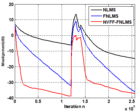
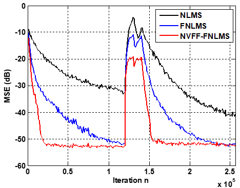
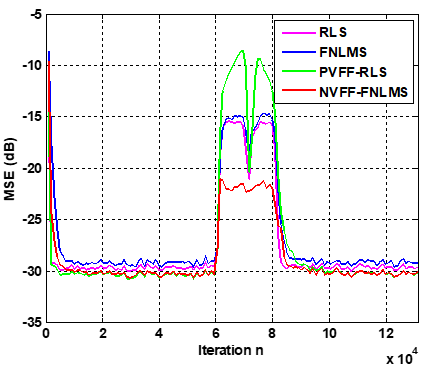
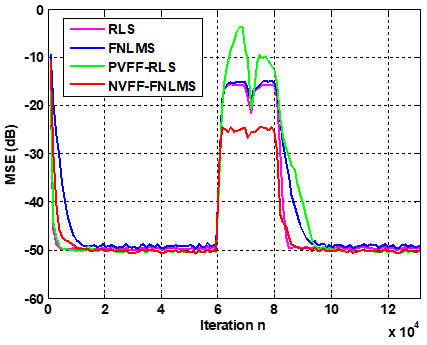
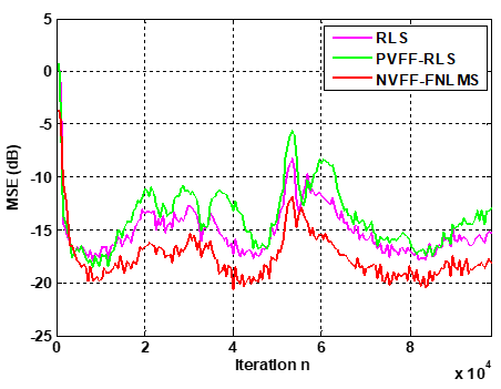
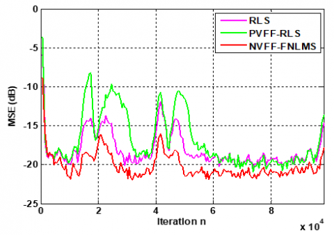
Figures 15 and 16 present the results of an evaluation comparing the proposed algorithm with classical RLS, FNLMS, and PVFF-RLS algorithms. Conducted at SNR values of 30dB and 50dB, this evaluation demonstrates the strong tracking performance of the proposed algorithm in a time-varying system. These excellent tracking behaviors stem from the effective adaptation of the proposed VFF to unknown system changes. Significantly, there is a substantial gain difference of approximately 13dB observed between NVFF-FNLMS and PVFF-RLS in a tracking scenario at SNR of 30dB, with a gain of approximately 20dB observed at SNR 50dB. Additionally, at SNR=30dB and SNR=50dB, the NVFF-FNLMS algorithm outperforms the RLS and FNLMS algorithms by about 7dB and 10dB, respectively.
Figure 15. Comparison of MSE evolution for USASI noise, $M=256, \mathrm{SNR}=30 \mathrm{~dB}, \varepsilon=0.01$
Figure 16. Comparison of MSE evolution for USASI noise, $M=256, \mathrm{SNR}=50 \mathrm{~dB}, \varepsilon=0.01$
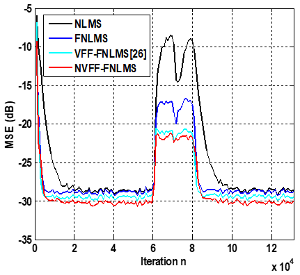
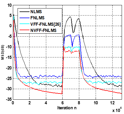
In the final experiment of this case, we evaluated the NVFF-FNLMS algorithm against the another recently VFF-FNLMS algorithm proposed by Bensouda and Benallal [26], The parameters for the VFF-FNLMS algorithm were configured as described by Bensouda and Benallal [26], as follow: ($\mu= \left.1, \lambda_{\min }=0.25, \lambda_{\max }=1, \beta=0.65, \beta_0=1.5, \sigma_{|e|}(0)=0\right)$. This comparison was carried out in a non-stationary system using USASI noise filtered with a 256-tap car impulse response and an SNR of 30dB. As illustrated in Figures 17 and 18, the NVFF-FNLMS surpasses the VFF-FNLMS in terms of tracking capability, demonstrating lower misalignment and achieving a slight improvement in the final MSE.
Figure 17. Comparison of MSE evolution for USASI noise, $M=256, \mathrm{SNR}=30 \mathrm{~dB}, \varepsilon=0.01$
Figure 18. Comparison of Misalignment evolution for USASI noise, $M=256, \mathrm{SNR}=30 \mathrm{~dB}, \varepsilon=0.01$
4.4.3 Case of a non-stationary input signal and stationary system
In this case, we conducted extensive experiments, as illustrated in Figures 19 and 20. The simulation results obtained using a non-stationary speech input signal with an impulse response length of $M=256$ and an SNR of 50dB, were evaluated based on MSE and misalignment criteria. These results unequivocally demonstrate that the proposed NVFF-FNLMS algorithm excels in echo attenuation and significantly outperforms both the NLMS and FNLMS algorithms. Specifically, the proposed approach exhibits superior performance in terms of steady-state MSE and achieves faster convergence speed. Furthermore, the results exhibit significantly improved accuracy and clarity, particularly in terms of misalignment, thereby demonstrating the superior performance of the NVFF-FNLMS algorithm compared to both the NLMS and FNLMS algorithms.
Figure 19. Comparison of MSE evolution for speech input, $M=256, \mathrm{SNR}=50 \mathrm{~dB}, \varepsilon=0.0001$
Figure 20. Comparison of misalignment evolution for speech input, $M=256, \mathrm{SNR}=50 \mathrm{~dB}, \varepsilon=0.0001$
4.4.4 Case of real experiment data
The measurements were carried out in a parallelepiped-shaped acoustic room with a reverberation time of about 180 ms. The background noise is below -20dB when the atmosphere of the surrounding rooms is relatively quiet. The sound system during the measurements consists of a table on which the sound recording microphone is mounted, a sound loudspeaker that radiates towards the speaker sitting in front of the microphone. Changes in the room acoustics or non-stationarities of the coupling acoustic channel are caused randomly (continuous movement in time with some short stops) by the horizontal or vertical movement of a rectangular metal plate (surface=60×40cm2) between the sound recording microphone and the loudspeaker. Depending on the speed of movement of the metal plate, the acoustic changes are considered to be: slow, medium or fast in time. The excitation signal at the loudspeaker output is a stationary-colored noise delivered by a standard signal generator. The signals captured at the loudspeaker and microphone inputs are digitized on 16 bits and stored with a sampling frequency of 8kHz. The simulation results are presented in Figures 21-23, corresponding to slow, medium, and fast variations, respectively, for an adaptive filter of size $M=512$ points. In Table 2, we find a summary of these results, where $M S E_{\min }$ is an average attenuation in decibels during the stationary phase and $M S E_{\max }$ represents the same performance but during the phase where the activity of the acoustic change is maximum. The performances $M S E_{\min }$ and $M S E_{\max }$ are calculated on an average of 512 consecutive samples. These results confirm the overall effectiveness and superior performance in terms of tracking capability of the proposed NVFF-FNLMS algorithm in real experimental data for multiple types of temporal variations. Our proposed algorithm offers an advantage in gains compared to PVFF-FNLMS algorithm of approximately 6dB in slowly varying systems, about 9dB in medium varying systems and 7dB in rapidly varying systems.
Figure 21. Tracking the slowly varying real acoustic impulse response, with $M=512, \varepsilon=0.0001$
Figure 22. Tracking the average varying real acoustic impulse response, with $M=512, \varepsilon=0.0001$
Figure 23. Tracking the rapidly varying real acoustic impulse response, with $M=512, \varepsilon=0.0001$
Table 2. Performance of the RLS, PVFF-RLS and proposed NVFF-FNLMS algorithms in real acoustic time-varying system
|
Algorithms |
Slow Variations |
Medium Variations |
Rapid Variations |
|||
|
|
$M S E_{\min }$ |
$M S E_{\max }$ |
$M S E_{\min }$ |
$M S E_{\max }$ |
$M S E_{\min }$ |
$M S E_{\max }$ |
|
RLS |
-8.28 |
-17.93 |
-11.92 |
-20.44 |
-6.45 |
-17.83 |
|
PVFF-RLS |
-5.65 |
-18.57 |
-7.35 |
-20.87 |
-2.53 |
- 17.23 |
|
NVFF-FNLMS |
-11.84 |
-20.66 |
-16.09 |
-21.98 |
-9.06 |
-20.21 |
4.5 VFF evolution
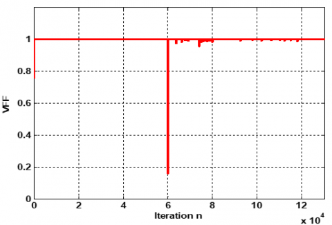
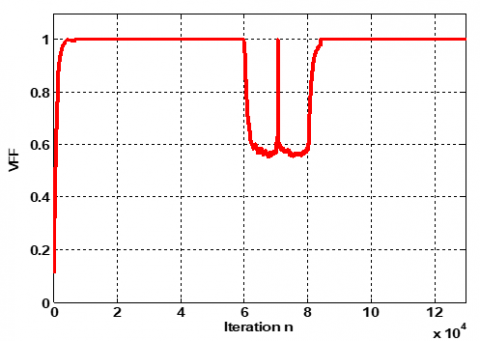
Figures 24 and 25 depict the temporal evolution of $\lambda(n)$ for the PVFF-RLS algorithm and our NVFF-FNLMS algorithm, respectively.
As observed from the curves, $\lambda(n)$ initially starts at a value below one prior to convergence and gradually approaches its maximum value of one during stationary periods. During system changes, the VFF of the proposed algorithm decreases significantly, enabling it to effectively track temporal variations in the unknown system. In contrast, the VFF of the PVFF-RLS algorithm exhibits difficulties in adapting to transient changes in the system. This observation explains the superior tracking performance of the proposed algorithm.
Figure 24. Evolution in time of $\lambda(n)$ of PVFF-RLS algorithm, with USASI input, in artificial non-stationary case, $\mathrm{SNR}=50$ and $M=256$
Figure 25. Evolution in time of $\lambda(n)$ of NVFF-FNLMS algorithm, with USASI input in artificial non-stationary case, $\mathrm{SNR}=50$ and $M=256$
4.6 Evaluation of computational complexity
In this section, we evaluate the computational complexities of the proposed NVFF-FNLMS algorithm with a comparison to the classical NLMS, RLS, FNLMS, and PVFF-RLS algorithms. The assessment relies exclusively on the count of arithmetic multiplications and divisions/square roots, with the results assessed and summarized in Table 3. Regarding the additional computational overhead introduced by the NVFFFNLMS the proposed NVFF-FNLMS algorithm requires $2 M+26$ multiplications and 5 divisions, compared to $2 M+$ 14 multiplications and 4 divisions for the conventional FNLMS. Thus, the exact increase is only 12 additional multiplications and one extra division per iteration. From a theoretical complexity perspective, this increase is marginal. For example, with filter lengths typically used in AEC (e.g., $M=512$ or $M=1024$), the overhead represents less than $2 \%$ of the total operations per iteration ( $\approx 1.16 \%$ for $M=$ 512 and $\approx 0.58 \%$ for $M=1024$). This confirms that the algorithm remains linear, i.e., $O(M)$, unlike RLS and PVFFRLS which exhibit quadratic complexity, $O\left(M^2\right)$.This difference arises because, beyond the raw arithmetic counts, the computation of the adaptive forgetting factor $\lambda(n)$ involves additional recursive updates and normalizations whose implementation cost is not fully captured by the simple operation counts.
For the memory requirements, the different algorithms can be analyzed as follows. For NLMS, the main variables to store are the input vector $\boldsymbol{x}(n)$ ($M$ elements), the weight vector $\widehat{\boldsymbol{w}}(n)$ ($M$ elements), and a few scalars such as $e(n), \mu_{N L M S}, C_{N L M S}$. This leads to a total memory of approximately $2 M$ i.e., linear in $M$. For FNLMS, in addition to $x(n)$ and $\widehat{\boldsymbol{w}}(n)$, an auxiliary vector $\tilde{\boldsymbol{c}}(n)$ (size $M$) is required, giving roughly $3 M$. Thus, compared to NLMS, the extra cost is limited to one additional vector of size $M$. In contrast, RLS requires storing the inverse correlation matrix $R^{-1}(n)\left(M^2\right.$ elements), together with $\boldsymbol{x}(n), \widehat{\boldsymbol{w}}(n)$, the gain vector $\boldsymbol{K}(n)$ (each of size $M$), and a few scalars. The total memory is therefore about $M^2+3 M$ dominated by the quadratic term $M^2$, which makes RLS impractical for large $M$.
For algorithms incorporating (VFF), the memory pattern depends on the underlying structure. PVFF-RLS inherits the quadratic complexity of RLS, with only a handful of additional scalar parameters, which are negligible compared to the dominant $M^2$ storage. On the other hand, the proposed NVFFFNLMS retains the linear memory profile of FNLMS. In addition to the $3 M$ elements already required by FNLMS, only about 12 extra scalar variables are stored, corresponding to averaged quantities used in the computation of the adaptive forgetting factor $\lambda(n)$ (e.g., $\varphi, \beta, \sigma_{|e|}, \sigma_d^2, \hat{\sigma}_y^2, \sigma_e^2$). Hence, the total memory of NVFF-FNLMS is approximately $\approx 3 M+12$, which remains $O(M)$ and practically identical to that of FNLMS.
Overall, both theoretical and empirical analyses confirm that the additional burden introduced by the NVFF mechanism is minimal. The computational overhead is limited to 12 multiplications and one extra division per iteration compared to FNLMS, and the memory increase is only a dozen scalars. These contributions are negligible relative to the dominant linear terms, confirming that NVFF-FNLMS maintains the $O(M)$ complexity and memory profile of NLMS and FNLMS, while avoiding the quadratic cost of RLS and PVFF-RLS. Consequently, the proposed algorithm remains highly suitable for practical real-time applications.
Table 3. Comparison of computational complexities
|
Algorithms |
Multiplications |
Divisions/Square Roots |
Memory |
|
NLMS |
$2 M+4$ |
1 |
2M |
|
FNLMS |
$2 M+14$ |
4 |
3M |
|
RLS [1] |
$4 M^2+4 M$ |
1 |
$M^2+3 M$ |
|
PVFF-RLS |
$4 M^2+4 M+14$ |
4/3 |
$M^2+3 M+10$ |
|
NVFF-FNLMS |
$2 M+26$ |
5 |
3M+12 |
In this paper, we introduced an enhanced FNLMS algorithm incorporating a novel VFF, termed the NVFF-FNLMS algorithm, specifically designed for AEC and System Identification (SI) applications. The proposed algorithm was comprehensively compared with the original NLMS, FNLMS, RLS, and PVFF-RLS algorithms, as well as the VFF-FNLMS and VSS-FNLMS algorithms, which also aim to improve tracking performance in time-varying systems. Performance evaluations demonstrate that the proposed NVFF-FNLMS algorithm outperforms classical FNLMS and NLMS algorithms in terms of tracking ability, steady-state MSE, convergence speed, and misalignment for both stationary and non-stationary signals and systems. Compared to previous VFF-FNLMS algorithms, the proposed NVFF-FNLMS exhibits superior tracking performance, achieving lower misalignment and a reduced final MSE.
The NVFF-FNLMS algorithm also demonstrates superior adaptability to both real and artificial time-varying systems compared to VFF-RLS algorithms, making it more suitable for non-stationary environments. Despite its performance gains, the NVFF-FNLMS algorithm remains computationally efficient compared to the more complex PVFF-RLS algorithm, making it a practical choice for real-time applications such as AEC.
While the proposed algorithm demonstrates significant improvements in convergence speed, tracking capability, and final MSE within the tested scenarios, certain limitations remain. Its applicability is constrained under conditions that have not yet been fully explored. In particular, the theoretical performance limits for tracking time-varying systems are not yet completely established, due to the lack of predictive models for varying rates of system change and distortions. Moreover, the NVFF-FNLMS algorithm may face limitations in scenarios involving two simultaneous systems (e.g., a time-varying system under double-talk conditions) or in environments characterized by strong impulsive noise.
Future work will aim to extend the theoretical analysis of tracking limits, enhance robustness under severe noise conditions, and develop hardware implementations (e.g., FPGA) to provide a more accurate assessment of real-time performance and facilitate integration into large-scale, real-world signal processing systems.
In conclusion, the NVFF-FNLMS algorithm proposed in this paper represents a practical, efficient, and effective solution for real-time applications such as AEC.
|
AEC |
Acoustic Echo Cancellation |
|
VFF |
Variable Forgetting Factor |
|
RLS |
Recursive Least Squares |
|
SI |
System Identification |
|
LMS |
Least Mean Square |
|
NLMS |
Normalized Least Mean Square |
|
FNLMS |
Fast NLMS |
|
FIR |
Finite Impulse Response |
|
FTF |
Fast Transversal Filter |
|
PVFF |
Practical Variable Forgetting Factor |
|
NVFF |
Novel Variable Forgetting Factor |
|
SNR |
Signal to Noise Ratio |
|
dB |
Decibel |
|
USASI |
United States of America Standards Institute |
|
WGN-AR20 |
White Gaussian Noise-Auto Regressive Process of order 20 |
|
Greek symbols |
|
|
$\lambda, \lambda_a$ |
forgetting factor |
|
$\mu$ |
Step-size |
|
$\gamma(n)$ |
likelihood variable |
|
$e_p(n)$ |
prediction error |
|
$a(n)$ |
variance of the forward error |
|
$\alpha, \beta$ |
weighting forgetting factor |
|
$\epsilon, \delta_0$ |
regularization parameters |
|
$\varphi$ |
constant that controls the variable forgetting factor |
|
$\zeta(n)$ |
variable convergence parameter |
[1] Uncini, A. (2015). Fundamentals of Adaptive Signal Processing. Switzerland: Springer International Publishing, pp. 287-347. https://doi.org/10.1007/978-3-319-02807-1
[2] Diniz, P.S.R. (2020). Fundamentals of Adaptive Filtering. In: Adaptive Filtering. Springer, Cham. https://doi.org/10.1007/978-3-030-29057-3_2
[3] Cutler, R., Saabas, A., Pärnamaa, T., Purin, M., Indenbom, E., Ristea, N.C., Aichner, R. (2024). ICASSP 2023 acoustic echo cancellation challenge. IEEE Open Journal of Signal Processing, 5: 675-685. https://doi.org/10.1109/OJSP.2024.3376289
[4] Hassani, I., Bendoumia, R., Guessoum, A., Abed, A. (2024). New variable selected coefficients adaptive sparse algorithm for acoustic system identification. Traitement Du Signal, 41(3): 1089-1099. https://doi.org/10.18280/ts.410301
[5] Venkata, S.K., Kishore, K.T. (2022). Speech enhancement for robust speech recognition using weighted low rank and sparse decomposition models under low SNR conditions. Traitement du Signal, 39(2): 633. https://doi.org/10.18280/ts.390226
[6] Benallal, A., Arezki, M. (2014). A fast convergence normalized least-mean-square type algorithm for adaptive filtering. International Journal of Adaptive Control and Signal Processing, 28(10): 1073-1080. https://doi.org/10.1002/acs.2423
[7] Ahmad, M.S., Kukrer, O., Hocanin, A. (2011). The effect of the forgetting factor on the RI adaptive algorithm in system identification. In ISSCS 2011-International Symposium on Signals, Circuits and Systems, Iasi, Romania, pp. 1-4. https://doi.org/10.1109/isscs.2011.5978751
[8] Wang, J. (2009). A variable forgetting factor RLS adaptive filtering algorithm. In Proceedings of the 2009 3rd IEEE International Symposium on Microwave, Antenna, Propagation and EMC Technologies for Wireless Communications, Beijing, China, pp. 1127-1130. https://doi.org/10.1109/MAPE.2009.5355946
[9] Song, S., Lim, J.S., Baek, S., Sung, K.M. (2000). Gauss Newton variable forgetting factor recursive least squares for time varying parameter tracking. Electronics Letters, 36(11): 988-990. https://doi.org/10.1049/el:20000727
[10] Leung, S.H., So, C.F. (2005). Gradient-based variable forgetting factor RLS algorithm in time-varying environments. IEEE Transactions on Signal Processing, 53(8): 3141-3150. https://doi.org/10.1109/tsp.2005.851110
[11] Cai, Y., de Lamare, R.C., Zhao, M., Zhong, J. (2012). Low-complexity variable forgetting factor mechanism for blind adaptive constrained constant modulus algorithms. IEEE Transactions on Signal Processing, 60(8): 3988-4002. https://doi.org/10.1109/TSP.2012.2199317
[12] Albu, F. (2012). Improved variable forgetting factor recursive least square algorithm. In 2012 12th International Conference on Control Automation Robotics & Vision (ICARCV), Guangzhou, China, pp. 1789-1793. https://doi.org/10.1109/icarcv.2012.6485421
[13] Paleologu, C., Benesty, J., Ciochina, S. (2014). A practical variable forgetting factor recursive least-squares algorithm. In 11th International Symposium on Electronics and Telecommunications (ISETC), Timisoara, Romania, pp. 1-4. https://doi.org/10.1109/isetc.2014.7010812
[14] Chu, Y.J., Chan, S.C. (2015). A new local polynomial modeling-based variable forgetting factor RLS algorithm and its acoustic applications. IEEE/ACM Transactions on Audio, Speech, and Language Processing, 23(11): 2059-2069. https://doi.org/10.1109/taslp.2015.2464692
[15] Lu, L., Zhao, H., Chen, B. (2016). Improved-variable-forgetting-factor recursive algorithm based on the logarithmic cost for Volterra system identification. IEEE Transactions on Circuits and Systems II: Express Briefs, 63(6): 588-592. https://doi.org/10.1109/tcsii.2016.2531159
[16] Song, Q., Mi, Y., Lai, W. (2019). A novel variable forgetting factor recursive least square algorithm to improve the anti-interference ability of battery model parameters identification. IEEE Access, 7: 61548-61557. https://doi.org/10.1109/access.2019.2903625
[17] Bouchard, M., Quednau, S. (2000). Multichannel recursive-least-square algorithms and fast-transversal-filter algorithms for active noise control and sound reproduction systems. IEEE Transactions on Speech and Audio Processing, 8(5): 606-618. https://doi.org/10.1109/89.861382
[18] Djendi, M. (2015). New efficient adaptive fast transversal filtering (FTF)-type algorithms for mono and stereophonic acoustic echo cancellation. International Journal of Adaptive Control and Signal Processing, 29(3): 273-301. https://doi.org/10.1002/acs.2470
[19] Paleologu, C., Benesty, J., Ciochină, S. (2014). A practical solution for the regularization of the affine projection algorithm. In 2014 10th International Conference on Communications (COMM), Bucharest, Romania, pp. 1-4. https://doi.org/10.1109/iccomm.2014.6866732
[20] Gazor, S., Liu, T. (2005). Adaptive filtering with decorrelation for coloured AR environments. IEE Proceedings-Vision, Image and Signal Processing, 152(6): 806-818. https://doi.org/10.1049/ip-vis:20045260
[21] Liu, J.C., Yu, X., Li, H.R. (2011). A nonparametric variable step-size NLMS algorithm for transversal filters. Applied Mathematics and Computation, 217(17): 7365-7371. https://doi.org/10.1016/j.amc.2011.02.026
[22] Slock, D.T. (1993). On the convergence behavior of the LMS and the normalized LMS algorithms. IEEE Transactions on Signal Processing, 41(9): 2811-2825. https://doi.org/10.1109/78.236504
[23] Mader, A., Puder, H., Schmidt, G.U. (2000). Step-size control for acoustic echo cancellation filters-An overview. Signal Processing, 80(9): 1697-1719. https://doi.org/10.1016/s0165-1684(00)00082-7
[24] Benesty, J., Paleologu, C., Ciochina, S. (2010). On regularization in adaptive filtering. IEEE Transactions on Audio, Speech, and Language Processing, 19(6): 1734-1742. https://doi.org/10.1109/TASL.2010.2097251
[25] Mengüç, E.C. (2020). Novel error variance estimation rule for nonparametric VSS-NLMS algorithm. Signal, Image and Video Processing, 14(7): 1421-1429. https://doi.org/10.1007/s11760-020-01691-7
[26] Bensouda, M.Y., Benallal, A. (2024). Improved Fast NLMS algorithm based on variable forgetting factor technique for acoustic echo cancellation. In Proceedings of the 8th International Conference on Image Signal Processing Applications (ISPA), Biskra, Algeria, pp. 1-6. https://doi.org/10.1109/ISPA59904.2024.10536798