Srilakshmi Chintapalli*![]() | Balasubadra Kandasamy
| Balasubadra Kandasamy![]()
© 2025 The authors. This article is published by IIETA and is licensed under the CC BY 4.0 license (http://creativecommons.org/licenses/by/4.0/).
OPEN ACCESS
The main goal is to develop a deep panoptic segmentation model specifically for medical image analysis, with an emphasis on recognizing common neurological disorders. The model aims to precisely identify and categorize various regions in brain scans by integrating sophisticated segmentation techniques with an autoencoder-based deep neural network, thereby aiding in the identification and diagnosis of neurodegenerative neurological disorders. This method has the potential to improve patient outcomes in neurological healthcare by increasing the accuracy of medical image interpretation. The proposed methodology is designed to provide precise and efficient automated detection and segmentation of neurological irregularities, including lesions in medical imagery using brain scan images. Valuable support to healthcare practitioners in their diagnostic and therapeutic efforts potentially in a web-based format for neurological disorders. The proposed model is aimed at supporting healthcare diagnosis by providing a reliable and effective system for the automatic recognition and categorization of neurological disorders using brain imaging techniques. By leveraging the specially designed U-NeuroSegNet infused with big data Spark processing, the model achieved exceptional accuracy and efficiency in identifying neurological abnormalities. In the proposed U-NeuroSegNet, the focus is on contributing significantly to advancements in neuro-oncology and personalized patient care ultimately benefiting individuals affected by neurological disorders. The study utilized large datasets of brain scan images. The U-NeuroSegNet model achieved an F1-score of 95.6%, a high accuracy of 98.2%, precision of 97.8%, sensitivity of 93.7%, and a recall rate of 98.0%. These results demonstrate the effectiveness of the U-NeuroSegNet model in accurately detecting neurological disorders, lesions, and tumors.
U-NeuroSegNet, panoptic segmentation, NIWatershed algorithm, intersection over union, accurate boundary detection, neurological disorders
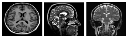
Neuroimaging has become an integral component of modern clinical practice, largely due to significant advancements in medical imaging technologies. It enables visualization of anatomical and physiological features that are otherwise hidden, allowing clinicians to extract imaging biomarkers and gather critical diagnostic information. This capability has revolutionized the field of radiology, contributing to improved diagnosis and patient care [1]. Several neuroimaging modalities are currently in use, including Magnetic Resonance Imaging (MRI), Magnetoencephalography (MEG), Electroencephalogram (EEG), Computed Tomography (CT), Diffusion Tensor Imaging (DTI), and Positron Emission Tomography (PET). Of these, MRI is the most frequently employed technique for identifying and evaluating neurological conditions. Neuroimaging is used both in clinical diagnostics and in neurological research, providing insights into the structural and functional aspects of the brain [2]. MRI stands out for its ability to generate high-resolution images with exceptional soft tissue contrast, making it a preferred method in neuroimaging. Unlike CT scans that utilize ionizing radiation, MRI uses powerful magnetic fields and radiofrequency pulses to produce images, offering a safer alternative with no radiation exposure [3]. MRI signal generation is influenced by two primary relaxation parameters: longitudinal relaxation time (T1) and transverse relaxation time (T2). T1 indicates the time it takes for protons to realign with the magnetic field after excitation, while T2 represents the time for protons to lose phase coherence. These distinct relaxation properties produce signal differences that contribute to image contrast [4]. MRI techniques are broadly categorized into Structural MRI (sMRI), which captures detailed anatomical features, and Functional MRI (fMRI), which maps brain activity. The brain can be viewed in multiple orientations—Axial, Coronal, and Sagittal planes—as depicted in Figure 1 [5].
Figure 1. MRI image
The study focuses on the implementation of panoptic instance segmentation for the automated analysis of medical images, particularly neurological conditions using brain scans. It involves a trained deep learning model designed to identify and precisely delineate neurological anomalies and lesions. The model provides real-time results enabling healthcare professionals to make faster and more accurate diagnoses [6]. The dataset sourced from Kaggle's public repository and the Chennai Brain and Spine Centre. This work employs deep learning algorithms specifically enhanced and modified U-Net is to analyse medical images and detect patterns indicative of various brain abnormalities. Existing manual analysis of medical images is labour-intensive and prone to human error [7]. To address these challenges, propose a panoptic segmentation model based on a modified U-Net to automate and improve the accuracy of identifying and segmenting neurological abnormalities in brain scans. This research highlights the critical importance of precise and efficient medical image analysis in neurology [8]. Neurological disorders such as lesions, require prompt diagnosis and meticulous delineation to facilitate effective treatment planning. The proposed approach utilizes deep learning methodology is to enhance automation and accuracy in identifying and segmenting neurological abnormalities [9]. This model represents a significant advancement in the domain of medical image analysis, contributing to improved diagnostic workflows and patient outcomes [10].
These diseases have been found to affect various parts of the nervous system and, in severe cases, can lead to dementia. Neurodegenerative diseases (NDDs) currently affect more than 50 million people worldwide, a number expected to rise to 130 million by 2050. NDDs typically manifest in individuals between the ages of 60 and 80. NDDs are generally diagnosed by comparing atypical symptoms and biomarker expressions against the patient’s medical history [11]. Since NDDs progress slowly, clinical symptoms often remain undetectable even after decades of neurodegenerative processes. As there are currently no effective drugs or therapeutic strategies to prevent or delay the progression of neurodegeneration, early diagnosis of NDDs with maximum accuracy is critical [12]. This research primarily focuses on the neurodegenerative diseases: Arnold Chiari malformation disease, Encephalocele disease, Ventriculomegaly, Holoprosencephaly, etc. The subsequent sections will provide an in-depth explanation of these diseases [13].
This research endeavor holds immense potential to significantly elevate the standard of care for patients grappling with neurological conditions. The initial exploration of this kind of initiative highlights the critical and meticulous role that medical imaging plays in neurology [14]. Conditions affecting the nervous system particularly within the brain require swift and precise diagnosis to inform and develop effective treatment strategies shown in Table 1. This approach automates and enhances the process of identifying and delineating neurological anomalies in brain scans [15]. This innovative research initiative promises to significantly improve the quality of healthcare services provided to individuals suffering from neurological disorders [16].
Table 1. The neurodegenerative disorders description
|
Neurodegenerative Disorders |
Description |
|
Arnold Chiari malformation |
Arnold Chiari malformation occur when brain tissues are pressed down to spinal cord due to skull being small at one side. This affects neuromuscular function. |
|
Arachnoid Cyst |
Arachnoid cysts are fluid-filled growths in the brain and spinal cord that, when they enlarge beyond 3cm or bleed internally, result in permanent damage to nerves. |
|
Cerebellah Hypoplasia |
Cerebellar hypoplasia is a congenital problem when cerebellum is small in size. Less than the 10th percentile of gestational age for cerebellar diameter is considered harmful. For instance, the average TPD measurements range from 16.6 mm to 23.1 mm at 20.4 weeks of gestation and from 32.2 mm to 41.6 mm at 31weeks of gestation |
|
Cisterna Magna |
Enlarged cerebellar region causes cisterna magna. It is a space in the posterior fossa dorsal to the medulla and caudal that is filled with cerebrospinal fluid. When larger than 10mm, they are usually dangerous causing neurological issues. |
|
Colphocephaly |
Colpocephaly is an uncommon genetic disorder characterized by lateral ventricle enlargement in two brain cavities. It is a congenital abnormality that results in the posterior brain ventricles growing larger than 10cc. |
|
Encephalocele |
A condition known as encephalocele results in brain tissue growing outside of a skull due to bone defect or any opening in skull causing neurological disorders. |
|
Holoprosencephaly |
When the human brain by birth is not predominately partitioned appropriately as right and left hemispheres people suffer from Holoprosencephaly problem and it is identified only in later stages of life. |
|
Hydranencephaly |
Hydranencephaly is an uncommon congenital condition in which there is no cerebral hemisphere. |
|
Ventriculomegaly |
Ventriculomegaly is a disorder where a build-up of cerebrospinal fluid (CSF) causes the brain to enlarge. Ventriculomegaly is categorized into mild, moderate, and severe based on the degree of enlargement. |
1.1 Problem statement
The early detection and accurate prediction of neurodegenerative neurological disorders—such as Arnold Chiari malformation, Cisterna Magna, Colphocephaly, Porencephaly, Ventriculomegaly—pose significant challenges due to the complex, progressive, and heterogeneous nature of these conditions. Existing diagnostic techniques largely depend on clinical assessments, neuroimaging, and biomarker evaluations, which are often invasive, time-intensive, and prone to subjective interpretation. Existing AI and machine learning models, while promising, face key limitations including inadequate handling of heterogeneous neuroimaging data, limited segmentation precision in distinguishing overlapping or diffuse brain regions, lack of scalability for large datasets, and insufficient integration with clinical workflows. Moreover, most models lack explainability restricts their utility in real-world medical settings. These critical gaps highlight the need for a robust, scalable, and interpretable deep learning-based segmentation framework that can efficiently process diverse brain imaging data and provide accurate, automated support for the diagnosis and monitoring of neurodegenerative neurological disorders.
1.2 Motivation
Neurodegenerative disorders such as Arnold-Chiari malformation, Cisterna Magna abnormalities, Colpocephaly, Porencephaly, and Ventriculomegaly pose significant and increasing challenges to patients, families, and global healthcare systems. These conditions are marked by a progressive deterioration in motor and cognitive abilities, often resulting in substantial disability, a decline in life quality, and rising demands for long-term medical and personal care. Timely and accurate diagnosis is essential to initiate treatment strategies that may help slow the progression and improve clinical outcomes. However, the subtle onset of symptoms and the drawbacks of existing diagnostic techniques—which are frequently invasive, time-intensive, and subject to interpretation—contribute to delayed or missed diagnoses, particularly in early stages.
Advancements in Artificial Intelligence (AI) and Machine Learning (ML) are offering new solutions to overcome these limitations. These technologies can process and interpret vast, multidimensional datasets from various sources such as neuroimaging, genetic information, and clinical records. By identifying intricate patterns and early biomarkers that traditional approaches may overlook, AI and ML support the development of more accurate, non-invasive, and scalable diagnostic systems. Predictive algorithms also have the capacity to flag individuals at risk before symptoms become clinically apparent, allowing for earlier intervention and personalized care planning. The pressing need to improve early detection methods, reduce diagnostic latency, and alleviate the societal impact of these diseases underscores the importance of AI-powered frameworks in transforming neurological care and integrating seamlessly into routine clinical workflows.
A novel Convolutional Neural Networks (CNN) model was developed for object identification and word segmentation for medical image analysis is presented for the identification and mapping of diseases' locations and regions are crucial for precise diagnosis. The utilization of computing and its practicality in medical advancements [17]. Employing computer vision and machine learning, extensive analysis was carried out for medical image analysis. The use of artificial intelligence and advanced neural networks in medical imaging was explored probably offering a detailed summary of the subject. Concentrated on contrasting CNNs and its application in various medical diagnostic tasks [18]. Addressed a new method for enhancing the adaptability of deep learning models for analyzing medical images. Their system consists of a collection of deep learning model parts and elements designed for specific tasks might simplify the creation and modification of AI models for different medical imaging activities [19]. This could lead to more customized answers and quicker adjustments to particular diagnostic requirements. Introduced E-Res U-Net for image segmentation, this model improved the accuracy of the model using ultrasonic muscle images. This model's structure was altered from the basic U-Net to enhance performance in three aspects, the dilated convolution component the E-Res layer and the E-Res [20].
Proposed a brand-new density-regression-based multi-scale convolutional UNet Multi-scale Contextual Attention (MSCA-UNet), and when compared it with other sophisticated density regression techniques, revealed two significant advances. The encoder component used an MSCA block with multi-scale interaction capabilities [21]. A dual-attention-based dense R-CNN model was presented. In this work involved a versatile and all-purpose instance segmentation framework Mask R-CNN. It can recognize objects in the image with good level of accuracy and produce superior segmentation labels for each occurrence [22]. To determine the performance of the designed CNN used AUC which tells how well the model can distinguish between classes across several thresholds. It showed the area under curve, assessed the accuracy of segmented regions compared with ground truth and showed how superficial it is compared to pixel accuracy [23]. To control side-effects of over-segmentation developed a neural network model retained only the minimum value of the objective area requiring edges of the object to be identified was safeguarded while the MRI image was being filtered and denoised [24].
The 3D UNet architecture proposed shows great potential as a volumetric segmentation tool, especially when applied to brain scans. It is possible to capture spatial information throughout the entire volume of the brain scans by extending the U-Net architecture into three dimensions. This is an important development for precise segmentation [25]. The work focused on the automatic classification of brain abnormalities using integration of VGG-16 NN technique with Fast R-CNN algorithm. Fast R-CNN is an improvement over the original R-CNN method designed for faster and more accurate object detection. It involves two main stages: generating region proposals and then classifying these proposals using a deep learning network [26]. Incorporating uncertainty quantification helps in understanding the reliability of the model’s predictions. This is crucial in medical imaging, where decisions based on automated segmentation need to account for potential variability and errors [27]. Proposed framework focused on segmenting brain abnormalities and other quantifying uncertainties in biomedical images, particularly useful for conditions such as traumatic brain injuries, stroke, and multiple sclerosis. Used whole brain imaging and a gray level confrontation matrix to build a deep k-means fuzzy CNN for the detection of glioma in brain scan images [28, 29].
A set of twelve Cohen class kernel functions processed EEG data for performing time frequency analysis. A feature vector containing modular energy values resulted from the data transformation process which was then provided to an Artificial Neural Network (ANN) classifier [30]. A new feature extraction method was created to handle time window observation variation through the optimum allocation approach [31]. The research applied Multiclass Least Square Support Vector Machine (MLS-SVM), which served to examine epileptic EEG signals; the application also monitored epileptic patient classification development. Researchers divided the classification process between partial and primary generalized epilepsy through the use of RBFNN and Multilayer Perceptron Neural Network (MLPNNs) [32].
A supervised clustering algorithm enables modeling historic clinical data which leads to predictions of patient survival based on the assigned cluster. Supervised learning strategies find combination with unsupervised learning through semi-supervised learning methods. Semi-supervised learning enhances limited labelled data by integrating additional unlabeled data to enable clustering (unsupervised) techniques which boost the classification (supervised) methods while employing additional data for predictive model regularization. In transductive learning, the test data serves as unlabeled input to enhance standard supervised classification approaches without causing data leakage, as the true labels remain unshared. This approach delivers improved outcomes, especially in scenarios with limited available labeled data.
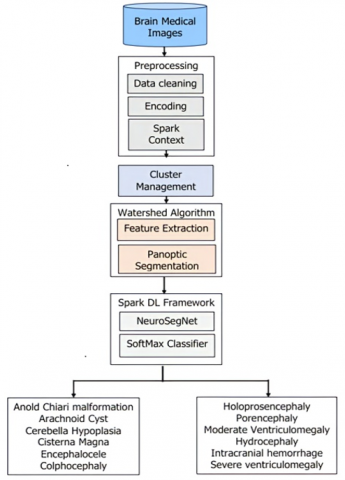
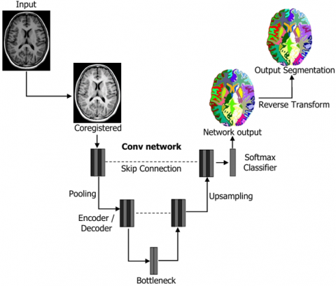
A Spark based DNN Model, U-NeuroSegNet Architecture, was specially designed for segmentation a modified Neuro-Intrinsic Watershed (NIWatershed) algorithm was utilized for the work done. Proposed system U- NeuroSegNet. When the neural network is fed with brain images as inputs, it classifies images by instances and identifies several classes of neurological abnormalities shown in Figure 2. The U-NeuroSegNet extracts relevant features from the input image and then projects them into segmentation masks. Spark is a data processing framework used for big data workloads that processes huge data sets using cluster computing. Spark Framework supports machine learning and big data processing in its engine. Using panoptic segmentation, which combines instance and semantic segmentation, created a unique U-NeuroSegNet to capture intricacy pixel by pixel. The proposed model utilized Apache Spark IDE for processing. In the Spark framework utilized Apache MXNet, it is a module in the framework that supports machine and deep learning processing. Automatic scaling is supported by multiple GPU servers and multi-node clusters. NVIDIA Spark framework supports accelerated computing through the RAPIDS component to support pipeline processing.
Figure 2. Apache Spark framework for NeuroSegNet
3.1 Dataset description
The dataset for U-NeuroSegNet is a comprehensive collection designed to support deep learning and big data-driven research in the detection and segmentation of neurodegenerative neurological disorders shown in Table 2. This combination provides a rich and diverse dataset consisting of approximately 10,500 patients. The imaging modalities used include both MRI and CT scans, capturing various perspectives and conditions relevant to neurological disorders. The dataset spans a wide age range from 20 to 85 years and maintains a relatively balanced gender distribution of approximately 52% male and 48% female. It encompasses a variety of neurodegenerative and neurological conditions, including Arnold Chiari malformation, Cisterna Magna, Colphocephaly, Porencephaly, Ventriculomegaly, and brain tumors, with cases representing both early and advanced stages of disease progression. Kaggle dataset offers a global mix of samples, while the medical center data reflects a more localized population. Several potential biases must be considered, such as limited representation of pediatric and very elderly populations, variations in imaging standards across institutions, and underrepresentation of certain ethnic groups. Planned subgroup analysis will evaluate model performance across different population segments to ensure fairness and robustness in real-world applications. Access is restricted to approved research institutions to maintain data security and ethical compliance and sample data’s shown in Table 3.
Table 2. Dataset description
|
Attribute |
Description |
|
Sources |
- Kaggle (public neuroimaging dataset) - Partner medical center (clinical brain scans) |
|
Modalities Used |
MRI and CT brain scans |
|
Total Subjects |
~10,500 patients (combined datasets) |
|
Age Distribution |
20–85 years |
|
Gender Distribution |
~52% Male, ~48% Female |
|
Disease Stages |
Early to advanced stages |
|
Geographic Representation |
- Kaggle: Mixed (global) - Medical center: Regional (single location) |
|
Potential Biases |
- Limited pediatric and elderly samples - Possible regional imaging standards - Underrepresentation of ethnic diversity |
|
Mitigation Strategies |
- Future inclusion of globally representative data - Subgroup performance analysis planned |
Table 3. Sample data
|
Patient ID |
Age |
Gender |
Modality |
Image Type |
Scan Size |
Tumor/Lesion Present |
Segmentation Mask |
|
P001 |
67 |
Male |
MRI |
T1-weighted |
256×256×150 |
No |
NA |
|
P002 |
72 |
Female |
MRI |
T2-weighted |
240×240×120 |
No |
NA |
|
P003 |
58 |
Male |
CT |
Axial |
512×512×80 |
Yes |
Provided |
|
P004 |
45 |
Female |
MRI |
FLAIR |
256×256×128 |
Yes (lesions) |
Provided |
|
P005 |
69 |
Female |
CT |
Coronal |
512×512×90 |
No |
NA |
3.2 Image pre-preprocessing
Preprocessing neuroimaging data is critical to ensure consistent, high-quality inputs for the deep learning model. The following steps outline the preprocessing pipeline for U-NeuroSegNet.
3.2.1 Noise reduction (Denoising)
Gaussian Filter for Noise Reduction: The Gaussian filter $G(i, j)$ is defined as:
$G(i, j)=\frac{1}{2 \pi \sigma^2} \exp \left(-\frac{i^2+j^2}{2 \sigma^2}\right)$ (1)
where, σ is the standard deviation of the Gaussian distribution, controlling the filter's smoothness. (i,j) are the spatial coordinates of the pixel. The kernel size typically depends on σ, with a larger σ leading to a larger kernel and more smoothing. To apply the Gaussian filter, we perform a convolution of the filter with the image X(i,j):
$X_{\text {denoised}}(i, j)=\sum_{x=-k}^k \sum_{y=-k}^k G(x, y) \cdot X(i+x, j+y)$ (2)
where, $X_{\text {denoised}}(i, j)$ is the denoised pixel value at position $(i, j) . X(i, j)$ is the original noisy image. $G(x, y)$ is the Gaussian kernel at the relative position $(x, y)$ from the pixel $(i, j). \mathrm{k}$ is the size of the kernel, typically $\mathrm{k}=\sigma \times 3$ times. This process smooths out high-frequency noise while preserving the image's structure.
3.2.2 Image resizing
Resizing images to a uniform size is essential in deep learning applications to ensure that the input dimensions match the model's requirements. A common technique for resizing images is bicubic interpolation, which uses a weighted average of the nearest 16 pixels (4×4 grid) for a higher quality result compared to bilinear interpolation. Bicubic Interpolation: The equation for bicubic interpolation is given by:
$X_{\text {resized}}\left(i^{\prime}, j^{\prime}\right)=\sum_{x=0}^3 \sum_{y=0}^3 w\left(x, i^{\prime}\right) \cdot w\left(y, j^{\prime}\right) \cdot X(i+x, j+y)$ (3)
where, $X_{\text {resized}}\left(i^{\prime}, j^{\prime}\right)$ is the resized pixel value at the new coordinates $\left(i^{\prime}, j^{\prime}\right) ; w\left(x, i^{\prime}\right)$ and $w\left(y, j^{\prime}\right)$ are the bicubic interpolation weights that are calculated based on the distance from the original pixel to the new pixel. $X(i, j)$ is the original image pixel value at position $(i, j)$. The sums over $x$ and $y$ range from 0 to 3 , as bicubic interpolation considers a 4×4 neighborhood of pixels. The bicubic interpolation weights $w\left(x, i^{\prime}\right)$ for each pixel are typically calculated using the following cubic spline function:
$w(t)=\left\{\begin{array}{lc}1-2|t|+|t|^3 & \text {for} 0 \leq|t|<1 \\ 4-8|t|+5|t|^2-|t|^3 & \text {for} 0 \leq|t|<1 \\ 0 & \text {otherwise}\end{array}\right.$ (4)
Noise Reduction (Gaussian Filter): Applies a Gaussian kernel to smooth the image and reduce high-frequency noise, improving the quality of medical images for analysis. Image Resizing (Bicubic Interpolation): Resizes the image to a fixed resolution while maintaining sharpness and minimizing distortion by using a weighted average of nearby pixels.
3.3 Data augmentation
Data augmentation is a crucial step in medical image processing, especially when working with neuroimaging data like MRI scans, to increase the diversity and size of the dataset. Since medical datasets can be limited, augmentation techniques help the model generalize better by introducing variations that preserve the underlying structure of the image. These variations might include transformations like rotation, scaling, flipping, and elastic deformations.
3.3.1 Rotation
It involves rotating the image by an angle $\theta$ to simulate different orientations.
$\left[\begin{array}{l}i^{\prime} \\ j^{\prime}\end{array}\right]=\left[\begin{array}{cc}\cos \theta & -\sin \theta \\ \sin \theta & \cos \theta\end{array}\right]\left[\begin{array}{l}i \\ j\end{array}\right]$ (5)
where, $\theta$ is the angle of rotation (usually between $-180^{\circ}$ and $\left.180^{\circ}\right) ;\left(i^{\prime}, j^{\prime}\right)$ are the coordinates of the rotated pixel. ( $i, j$ ) are the original pixel coordinates. By applying this transformation to the whole image, each pixel is repositioned based on the rotation angle, allowing the network to learn from different perspectives of the brain structures in neuroimaging.
3.3.2 Flipping
It is a simple and effective augmentation method, especially flipping images horizontally or vertically. Horizontal flipping is represented by:
$X_{\text {flipped}}(i, j)=X(W-i, j)$ (6)
where, $W$ is the width of the image. $X_{\text {flipped}}(i, j)$ is the pixel value after horizontal flipping. $X(i, j)$ is the original image pixel value at coordinates ($i, j$). Similarly, vertical flipping can be done by reflecting the image along the vertical axis.
$X_{\text {flipped}}(i, j)=X(i, H-j)$ (7)
where, H is the height of the image. This transformation swaps the pixel values in a vertical manner. Flipping images helps the model learn from different mirrored perspectives, which is crucial in tasks like brain lesion segmentation, where spatial orientation is not fixed.
3.3.3 Scaling (Resizing)
It alters the size of the image, either by zooming in or out, which simulates varying levels of focus or distances. The scaling transformation is represented by:
$X_{\text {scaled}}\left(i^{\prime}, j^{\prime}\right)=X\left(\delta_i. i, \delta_j. j\right)$ (8)
where, $X_{\text {scaled}}\left(i^{\prime}, j^{\prime}\right)$ is the pixel value at the scaled coordinates. $\delta_i(i)$ and $\delta_j(j)$ are scaling factors in the i and j directions. ( $i, j$ ) are the original pixel coordinates. Scaling can help the model learn spatial invariance, ensuring the model recognizes structures irrespective of their size in the image.
3.3.4 Elastic deformation
Introduces random deformations in the image, mimicking the variability found in biological tissues, such as the brain's elasticity. This method is particularly useful in neuroimaging as it preserves anatomical structures while introducing more variability. The deformation can be represented by the following equation:
$\left.X_{\text {deformed}}\left(i^{\prime}\right)=X\left(i+\delta_i(i)\right), j+\delta_j(j)\right)$ (9)
where, $X_{\text {deformed}}\left(i^{\prime}\right)$ is the pixel value after applying the deformation. $\delta_i(i)$ and $\delta_j(j)$ are random displacements based on a Gaussian distribution. The displacement fields $\delta_i(i)$ and $\delta_j(j)$ are usually generated from a random noise field, and their values are scaled based on the desired magnitude of deformation. Elastic deformations simulate slight distortions in the neuroimaging data, allowing the model to learn more generalized features and improve robustness to such variations.
3.3.5 Brightness and contrast adjustments
Adjusting the brightness and contrast of images helps simulate different imaging conditions. The pixel intensities can be modified as follows:
Brightness Adjustment:
$X_{\text {brightened}}(i, j)=X(i, j)+\Delta X$ (10)
where, $\Delta$ is a constant added to all pixel intensities to adjust the brightness.
Contrast Adjustment:
$X_{\text {contrasted}}(i, j)=\alpha \cdot(X(i, j)-\mu)+\mu$ (11)
where, $\alpha$ is the contrast scaling factor (typically $\alpha>1$ for increasing contrast). $\mu$ is the mean intensity value of the image. $X_{\text {contrasted}}(i, j)$ is the adjusted pixel value.
Brightness and contrast adjustments help the model learn from variations in the image quality due to different scanners or acquisition conditions.
3.3.6 Shearing
It involves applying a shear matrix that distorts the image in one direction, typically along the horizontal or vertical axis. The equation for horizontal shearing is:
$\left[\begin{array}{l}i^{\prime} \\ i^{\prime}\end{array}\right]=\left[\begin{array}{ll}1 & \lambda \\ 0 & 1\end{array}\right]\left[\begin{array}{l}i \\ j\end{array}\right]$ (12)
where, $\lambda$ is the shear factor, controlling the amount of distortion. ($i^{\prime}, j^{\prime}$) are the transformed pixel coordinates. $(i, j)$ are the original coordinates. Shearing helps simulate perspective shifts in the images, which may occur due to different angles of data collection or movement of the subject.
These data augmentation methods significantly enhance the model's ability to generalize, improving performance in detecting and segmenting neurodegenerative neurological disorders from neuroimaging datasets.
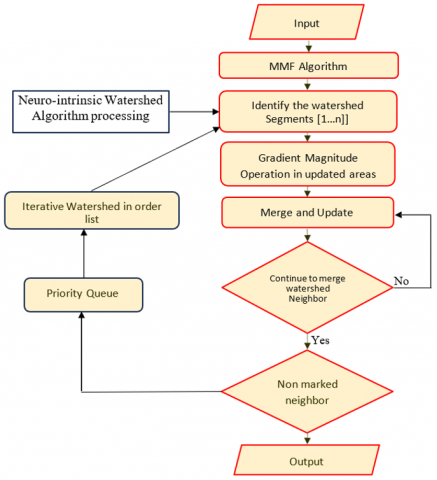
3.4 NIWatershed algorithm
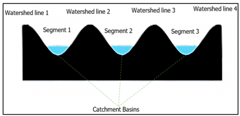
The modified NIWatershed algorithm is a technique used for image segmentation, particularly for separating overlapping objects or regions. NIWatershed algorithm is utilized to segment the brain images into individual regions or components, facilitating the identification and analysis of distinct anatomical structures and pathological abnormalities shown in Figure 3. NIWatershed Algorithm has been utilized to address challenges such as heterogeneity and irregular shape can complicate existing segmentation approaches. By applying the algorithm to preprocessed brain scan images, we were able to effectively partition the regions, enabling precise measurements of volume and facilitating quantitative analysis of abnormalities.
Figure 3. Watershed basins
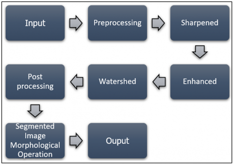
NIWatershed algorithm is a variation of the classical Watershed algorithm for segmenting brain scan images. The algorithm treats pixel intensities as a terrain where higher intensities represent peaks and lower intensities represent valleys shown in Figure 4. The algorithm then "floods" the map from the valleys (pixels with the lowest intensities) and lets the watershed markers converge at the peaks (pixels with the highest intensities). If refinement of bounding regions is necessary NIWatershed algorithm auto-adjusts the bounds. Once the U-NeuroSegNet predicts potential bounding boxes for objects in an image, the NIWatershed algorithm can be applied to better separate objects that are close together or overlapping conveniently which helps in increasing accuracy effectively. NIWatershed Segmentation works by grouping pixels based on similar intensities. It separates the abnormal region from the rest of the normal region of the brain scan image shown in Figure 5. The NIWatershed Segmentation is a morphological operation to double-check the predicted output.
The NIWatershed Segmentation algorithm is an advanced technique used to segment regions of interest in neuroimaging data, such as MRI scans by identifying and isolating specific structures, lesions, or abnormalities related to neurodegenerative disorders (e.g., Arnold Chiari malformation, Arachnoid Cysts). The Watershed algorithm is inspired by the topographic analogy of a watershed, where the image intensity is treated such as landscape, and "flooding" is simulated to identify regions of interest. The NIWatershed algorithm incorporates normalized intensity values to improve segmentation accuracy, especially for medical images where intensity distributions can vary due to different acquisition methods or conditions.
Figure 4. NIWatershed processing
Figure 5. NIWatershed algorithm processing
3.5 Algorithm of Watershed segmentation
3.5.1 Step 1: Pre-processing of image
Before applying the Watershed algorithm, an initial pre-processing step is required to enhance the contrast and remove noise, ensuring the features are well-defined. Common pre-processing steps include smoothing (Gaussian filtering), histogram equalization, and noise reduction.
Gaussian filtering:
$X_{\text {smoothed}}(i, j)=\sum_{x=-k}^k \sum_{y=-k}^{k 3} G(x, y) \cdot X(i+x, j+y$ (13)
where, $G(x, y)$ is the Gaussian kernel, and $X(i, j)$ is the original image.
3.5.2 Step 2: Gradient calculation
The next step involves computing the gradient of the image. The gradient magnitude is used to identify the boundaries of regions (edges). In the context of neuroimaging, these gradients highlight boundaries between different brain regions or lesions. The gradient of an image $X(i, j)$ is computed as:
$\boldsymbol{G}(\boldsymbol{x}, \boldsymbol{y})=\sqrt{\left(\frac{\partial X}{\partial i}\right)^2+\left(\frac{\partial X}{\partial j}\right)^2}$ (14)
3.5.3 Step 3: Normalization of intensity
Normalizing the intensity values is crucial to reduce the impact of varying intensities from different imaging conditions. The normalized intensity $X_{\text {norm}}(i, j)$ at each pixel can be calculated as:
$X_{\text {norm}}(i, j)=\frac{X(i, j)-X \min }{X \max -X \min }$ (15)
where, $\min (\mathrm{X})$ and $\max (\mathrm{X})$ are the minimum and maximum intensity values of the X, respectively. In this expression, Xmin and Xmax represent the lowest and highest intensity values found in matrix.
This normalization ensures the intensity values are scaled to a [0, 1] range, making it easier for the watershed algorithm to distinguish between different intensity regions.
3.5.4 Step 4: Watershed transformation
The algorithm "floods" this surface starting from low points (local minima) and grows regions until boundaries (edges) are reached.
The flooding process can be modeled as:
$X_{\text {watershed}}(i, j)=\operatorname{argmin}_r(\operatorname{dist}(X(i, j), r)$ (16)
where, $r$ represents regions of the image, which start from seed points; $\operatorname{dist}(X(i, j), r)$ measures the distance between the pixel's intensity $X(i, j)$ and the region's intensity r. The flooding process continues until all pixels are assigned to a region, and boundaries are formed based on the intensity gradients.
3.5.5 Step 5: Markers and seed point initialization
The algorithm requires markers or seed points to initiate the watershed process. These markers typically correspond to areas of high interest, such as a lesion or a specific anatomical region in the brain (e.g., gray matter, white matter). Markers can be placed manually, or an automatic method (like thresholding) can be used to select initial points:
$\begin{gathered}\operatorname{Marker}(i, j)= \left\{\begin{array}{l}1, \text {if pixel belongs to foreground} \\ 0, \text {otherwise}\end{array}\right.\end{gathered}$ (17)
3.5.6 Step 6: Segmentation and region labelling
After the flooding process, each pixel will be assigned to a specific region, labelled according to the watershed labels. The output of the watershed algorithm is a segmented image $X_{\text {seg}}(i, j)$ where distinct regions corresponding to different brain structures or abnormalities are separated. The segmentation result can be represented as:
$X_{\text {seg}}(i, j)=$ region label at $(i, j)$ (18)
where, each region corresponds to a specific anatomical or pathological feature (e.g., a lesion or an area of atrophy).
|
Pseudo Code |
|
Input: Original Image I(x, y) Preprocess image using Gaussian filter Compute gradient G(x, y) Normalize image intensity I_norm(x, y) Generate markers (seeds) for watershed (could be based on thresholding) Apply Watershed transformation: For each pixel (x, y): Compute flooding distance and assign to region based on intensity gradient Assign regions based on flooding process and boundary detection Output: Segmented image I_seg(x, y) with labeled regions |
The NIWatershed Segmentation Algorithm for Neurodegenerative Neurological Disorders relies on the concept of watershed flooding applied to normalized intensity images to identify regions of interest, such as lesions or atrophied areas in neuroimaging data. It includes preprocessing, gradient computation, intensity normalization, and region labeling steps. The algorithm's mathematical basis involves gradient and intensity calculations, normalization, and region labeling, making it suitable for the segmentation of complex medical images such as MRIs in the diagnosis and study of neurodegenerative diseases.
3.6 Panoptic segmentation
A comprehensive strategy that combines instance and semantic segmentation referred to as panoptic segmentation. Semantic segmentation offers an in-depth knowledge of the discrete characteristics found in brain images, while instance segmentation assigns a distinct label to each pixel. Object detection and segmentation are merged into a single, cohesive framework through panoptic segmentation. With this technique, regions of interest are identified using the output of an object detector, and object boundaries are then precisely delineated using a segmentation module.
3.6.1 IoU and ABD in panoptic segmentation
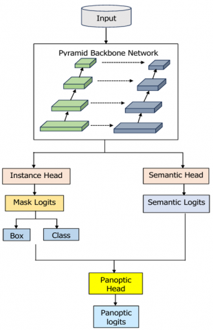
The proposed model, NeuroSegNet uses panoptic segmentation shown in Figure 6. The two most important factors affecting panoptic segmentation are Intersection over Union and Accurate Boundary Detection. The confidence score over the projected bounding box and predicted object class is directly impacted by the intersection over union. A modified edge detection technique is used for Accurate Boundary Detection (ABD) to predict boundaries with high precision.
3.6.2 Panoptic segmentation is dependent on ground truth
For complex tasks of panoptic segmentation, it requires solid Ground Truth data. The training images have been accurately annotated to indicate the exact boundaries of objects. The model uses this for testing its output predictions against the ground truths to decide and improve accuracy.
Figure 6. Flow of panoptic segmentation
Figure 7. Neuro intensive lightweight panoptic segmentation
Panoptic segmentation uses Gaussian filters with Laplacian transformation for edge detection, shown in Figure 7. This is particularly useful in medical imaging for tasks such as the identification of specific regions in the brain or lesions related to neurodegenerative disorders. The ground truth in the context of panoptic segmentation is manually annotated data that provides the true label for each pixel in an image. For effective training and evaluation, the ground truth must contain both semantic and instance-level annotations. In panoptic segmentation, the ground truth is typically represented in the following format:
$G T_{\text {panoptic}}=\left\{\left(p_x, C_x, r_x\right)\right\}$ (19)
where, $p_x$ represents the pixel positions in the image; $C_x$ is the semantic class label assigned to pixel $p_x$ (e.g., "lesion," "gray matter," etc.). $r_x$ is the instance-specific label, distinguishing between different objects of the same class (e.g., lesion 1 , lesion 2).
Semantic Segmentation Ground Truth: For semantic segmentation, the ground truth is a map where each pixel is assigned a class label:
$G T_{\text {semantic}}(i, j)=C(i, j)$ (20)
where, $G T_{\text {semantic}}(i, j)$ is the class label at pixel $(i, j) ; C(i, j)$ is the class label for the pixel at position $(i, j)$; such as "background," "lesion," "gray matter," etc.
Instance Segmentation Ground Truth: In instance segmentation, each object (or region of interest) in the image needs to be labeled separately, even if they belong to the same class. This is done using a unique instance ID $G T_{\text {instance}}(i, j)$.
$G T_{\text {instance}}(i, j)=r(i, j)$ (21)
An instance label that distinguishes between different objects of the same class.
3.6.3 Panoptic segmentation loss function
In panoptic segmentation, the loss function is typically a combination of losses for semantic segmentation and instance segmentation. The overall loss $L_{\text {panoptic}}$ can be defined as:
$L_{\text {panoptic}}=\lambda_{\text {semantic}} L_{\text {semantic}}+\lambda_{\text {instance}} L_{\text {instance}}$ (22)
where, $L_{\text {semantic}}$ is the loss associated with semantic segmentation (e.g., cross-entropy loss between predicted and ground truth class labels); $L_{\text {instance}}$ is the loss associated with instance segmentation (e.g., a distance-based loss between predicted and ground truth instance .labels). $\lambda_{\text {semantic}}$ and $\lambda_{\text {instance}}$ re-balancing weights for the semantic and instance segmentation losses.
Semantic Loss Function: The semantic loss can be expressed as:
$\begin{gathered}L_{\text {semantic}}= -\sum_{i, j} \sum_{C_x \in C} 1_{\left\{C_x=C(i, j)\right\}} \log p\left(C_x \mid X(i, j)\right)\end{gathered}$ (23)
where, $C$ is the set of all possible class labels. $1_{\left\{C_x=C(i, j)\right\}}$ is the indicator function that is 1 if the class $C_x$ matches the class label at pixel ($i, j$); $p\left(C_x \mid X(i, j)\right)$ is the predicted probability of class $C_x$ for the pixel $(i, j)$.
Instance Loss Function: For instance, segmentation, a typical loss function involves the prediction of unique instance labels and boundaries. A common approach is the Hungarian algorithm for instance matching, and the loss can be defined as:
$L_{\text {instance}}=\sum_{x=1}^N \sum_{i, j}\left(\left\|X_{\text {pred}}(i, j)-X_{g t}(i, j)\right\|^2\right)$ (24)
where, $X_{\text {pred}}(i, j)$ is the predicted instance label at pixel $(i, j)$; $X_{g t}(i, j)$ is the ground truth instance label at pixel $(i, j) ; \mathrm{N}$ is the total number of instances.
3.6.4 Evaluation metrics for panoptic segmentation
To evaluate the performance of a panoptic segmentation model, various metrics are used. The two main components are semantic segmentation accuracy and instance segmentation accuracy.
Panoptic Quality (PQ): The Panoptic Quality metric combines both segmentation and instance accuracy:
$P Q=\frac{1}{|P|} \sum_{p \epsilon P} \frac{\left|T P_p\right|}{\left|G T_p\right|+\left|F P_p\right|}$ (25)
where, $P$ is the set of panoptic predictions. $T P_p, F P_p$, and $G T_p$ are the true positives, false positives, and ground truth pixels in panoptic prediction ppp, respectively.
Semantic Accuracy (mIoU): Mean Intersection over Union (IoU) for semantic segmentation:
$m I o U=\frac{1}{|C|} \sum_{C_x \in C} \frac{\mid G T_{C_x} \cap \text {Pred}_{C_x} \mid}{G T_{C_x} \cup \text {Pred}_{C_x}}$ (26)
where, C is the set of semantic classes. $G T_{C_x}$ and $\operatorname{Pred}_{C_x}$ are the ground truth and predicted regions for class $C_x$.
Instance Segmentation Quality (SQ): Measures the instance-level accuracy:
$S Q=\frac{1}{|X|} \sum_{x \in X} \frac{\left|T P_x\right|}{\left|G T_x\right|+\left|F P_x\right|}$ (27)
where, $X$ is the set of instances. $T P_x, F P_x$, and $G T_x$ are the true positives, false positives, and ground truth pixels for instance $x$, respectively.
The ground truth in panoptic segmentation involves both semantic and instance-level annotations. Panoptic segmentation aims to provide a comprehensive segmentation map by assigning both class labels and instance IDs to each pixel. The ground truth equations define how these labels are assigned, and the loss functions and evaluation metrics ensure that the model can be trained and assessed for both aspects. These methods are particularly useful in medical imaging tasks, such as segmenting and identifying lesions or other areas affected by neurodegenerative disorders.
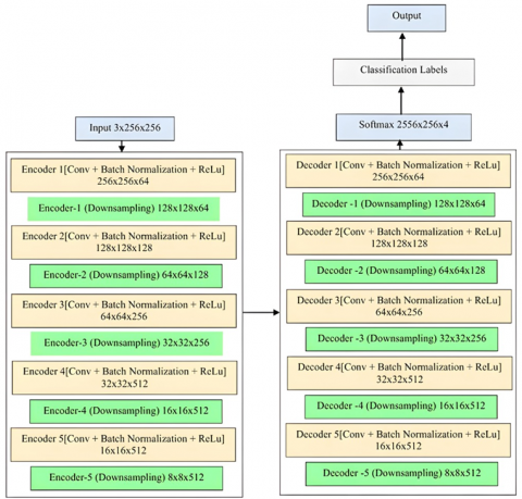
3.7 U-NeuroSegNet encoder/decoder
The U-NeuroSegNet comprises an encoder-decoder network structure augmented with skip connections, which play a vital role in preserving spatial information throughout the segmentation process. In proposed U-NeuroSegNet is based on the principle of the encoding and decoding process. The encoder in U-NeuroSegNet extracts detailed features from the input medical image, capturing relevant patterns indicative of abnormalities presence. Subsequently, the decoder reconstructs the segmented output, utilizing the extracted features to delineate boundaries accurately. While no specific formula governs this process, the architecture's design incorporates principles related to convolutional operations, skip connections, and activation functions to facilitate effective brain segmentation.
3.7.1 Subnet division
It involves dividing the neural network architecture into smaller, manageable subnetworks. Divide the neural network into multiple subnetworks to facilitate parallel processing and optimize computational efficiency.
3.7.2 Category brain slicing
This method focuses on segmenting the brain into different categories or regions based on specific criteria. Categorically, brain slicing is used to partition the brain images into distinct regions corresponding to different anatomical structures and pathological features, aiding in the accurate detection and classification of brain images.
3.7.3 Narrow object region
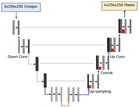
Narrow object region detection aims to identify and delineate small or thin structures within the images. This method is employed to detect narrow regions within the brain images that correspond to abnormality boundaries or blood vessels, enabling precise segmentation and analysis. The reason why encoder and decoders are relevant to designing Deep U-NeuroSegNet is that output results must have the same dimension as the input. In the Panoptic Segmentation task done ensures output image Pyramid Backbone Network Input Instance Head Semantic Head Semantic Logits Mask Logits Box Class Panoptic Head Panoptic logits is of same dimension as the original input. Proposed DeepU-NeuroSegNet uses a modified panoptic segmentation that is suitable for ultrasound images. The neural network is fed brain scan images as inputs, and classifies objects pixel by pixel.
Figure 8. U-NeuroSegNet architecture
In the encoder-decoder architecture all pixels are classified as abnormal/normal. The encoder takes the required features from images shown in Figure 8. The encoder contains conv layers, Relu and Maxpool to extract relevant features for each class. The decoder creates feature maps and takes the extracted vectors and reconstructs a segmentation mask. Skip Connection is added to decoder to ensure decoder works with specific features rather than general ones. The loss function is an intrinsic cross-entropy loss function used in the U-NeuroSegNet model to compare the predicted output for each class against the ground truth value.
Loss $=-\sum_n \operatorname{grtruth}(k) \odot \log \left(\operatorname{softmax}\left(Z_k\right)\right)$ (28)
where, $\operatorname{grtruth}(k)$ represents the ground truth value for class k . $\odot$ is the element-wise multiplication operator. $\operatorname{softmax}\left(Z_k\right)$ is the predicted probability distribution for class k generated by the softmax function. Here, $Z_k$ represents the raw scores (logits) from the neural network before applying the softmax function. The softmax function calculates the probability distribution for each class by normalizing the logits across all n classes:
$\operatorname{softmax}\left(Z_k\right)=\frac{\exp \left(Z_k\right)}{\sum_{y=1}^n \exp \left(Z_y\right)}$ (29)
where, $Z_k$ is the score for class k (logit). n is the number of classes. The denominator normalizes the exponentiated logits to give a probability distribution across all classes.
This loss function helps the model adjust its weights and improve accuracy by penalizing incorrect predictions based on the difference between the predicted probability and the ground truth. In U-NeuroSegNet the dice loss is a loss function that weighs the imbalance between the intersection area and total area in similar kind of images. The dice loss will be less when dice coefficient is high. Dice loss represents the imbalance in segmentation mask. The $\Psi$ represents the smoothing factor and is used both in numerator and denominator. The combined Cross-Entropy Loss and Dice Loss function is expressed as:
Loss $=2 \sum_n\left(\right.$ softmax $\left(Z_k\right) \odot$ grtruth $(k)+$ Dice Loss $)$ (30)
where, $\operatorname{softmax}\left(Z_k\right)$ is the predicted probability distribution for class k generated by the softmax function. grtruth($k$) is the ground truth for class k. The Dice Loss is added to penalize the difference between the predicted segmentation mask and the ground truth mask. The Dice similarity coefficient is commonly used to measure the overlap between two sample sets. It is defined as:
Dice Loss $=1-\frac{2 \sum_{l=1}^n \operatorname{grtruth}(k) \odot \operatorname{softmax}\left(Z_k\right)}{\sum_{l=1}^n \operatorname{grtruth}(k)+\sum_{l=1}^n \operatorname{softmax}\left(Z_k\right)}$ (31)
$S_n(i)=\frac{\exp (f m(i))}{\sum_{l=1}^n \exp \left(f m_k(i)\right)}$ (32)
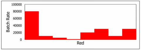
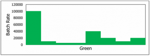
where, $S_n(i)$ represents the probability of class n for the pixel x. $f m(i)$ is the feature map function at position i for the $\mathrm{k}_m^{\text {th}}$ class. The sum in the denominator is the normalization factor ensuring that the probabilities for all classes sum to 1, and the feature map function $f m(i)$ corresponds to the activation function output for the pixel at position i. Proposed model also features an innovative mechanism for weight pre-computation based on the pixel frequency across the different classes in the training dataset. This pre-processing strategy helps the model to focus more effectively on class imbalances during training, enabling better segmentation performance for underrepresented classes. The equation for the modified morphological operation in U-NeuroSegNet is given as:
$\begin{aligned} \Omega(x)=\Omega_C(x)+ & \Omega_0 \log \left(\frac{1}{2} \int_{-\infty}^{\infty}\left[K_1(I)\right.\right. \left.\left.-K_2(I)\right]^2 d \zeta\right)\end{aligned}$ (33)
where, $\Omega(x)$ is the precomputed weight for pixel x in the image. $\Omega_C(x)$ represents the weight map for pixel $\mathrm{x}. \Omega_0$ is a constant that acts as a scaling factor for the precomputed weight. $K_1(I)$ is the distance to the nearest pixel's border, which refers to the proximity to the nearest boundary of a specific object or structure within the image. This is associated with the pixel I. $K_2(I)$ represents the distance to the second closest pixel's border, which helps in determining separation between different regions or objects within the image. $\zeta$ is the integration variable, indicating the spatial relationship between the pixels being considered in the morphological operation. $\mathrm{d} \zeta$ represents the differential element of integration over the entire spatial domain of the image.
This morphological operation is key to adjusting the weights based on the distances between pixels and their separation borders in the image shown in Figure 9. By computing the distance to the nearest and second-nearest borders, the model can assign higher weights to pixels near object boundaries, which are often the most critical for accurate segmentation. The logarithmic term and the scaling factors are designed to refine these weight adjustments, enabling the model to focus more on important regions while suppressing less relevant ones. This operation enhances the U-NeuroSegNet model's ability to identify specific structures and conditions in neurodegenerative neurological disorder images by emphasizing the correct regions and improving segmentation accuracy.
Algorithm
The U-NeuroSegNet algorithm is a Deep Learning and Big Data-Driven Panoptic Segmentation framework specifically designed for identifying specific conditions in neurodegenerative neurological disorders. Below is a high-level description of the algorithm, broken into key stages:
Step 1: Data preprocessing
Step 1.1: Image acquisition: Collect neuroimaging data such as MRI, Ultrasound, CT, or PET scans related to neurodegenerative disorders (e.g., the dataset should include both labeled ground truth data and images corresponding to the various stages of neurodegenerative conditions.
Step 1.2: Noise Reduction: Apply Gaussian filters or Median filters to remove any noise from the images.
$G(i, j)=\frac{1}{2 \pi \sigma^2} \exp \left(-\frac{i^2+j^2}{2 \sigma^2}\right)$ (34)
where, σ is the standard deviation that controls the filter's strength.
Step 1.3: Resizing: Standardize the image size for the neural network by resizing all images to a fixed size W×H times. Use interpolation techniques like bilinear interpolation for resizing.
Step 1.4: Normalization: Normalize pixel values to a range between 0 and 1 or mean-variance normalization to enhance learning. For each pixel p:
Figure 9. U-NeuroSegNet processing
$p^{\prime}=\frac{p-u}{\sigma}$ (35)
where, μ is the mean pixel value and σ is the standard deviation of the pixel values.
Step 1.5: Data augmentation: Apply augmentation techniques such as rotation, flipping, and scaling to diversify the dataset. This ensures that the model generalizes better and avoids overfitting.
Step 2: U-Net architecture setup (encoder-decoder structure)
Step 2.1: Contracting path (encoder): The contracting path consists of multiple convolutional layers followed by a ReLU activation function and max pooling for down-sampling. The number of filters is doubled at each down-sampling step.
Bottleneck Layer 2.2: A central layer between the contracting and expansive paths. Contains bottleneck convolutions that help in better feature extraction from complex patterns.
Expanding Path (Decoder) 2.3: The expanding path consists of up-sampling and convolutions. Uses skip connections from the contracting path to provide better localization information.
Convolutional Layer 2.4: Apply 3×3 convolutions with a ReLU activation function after each layer in the encoder and decoder. Use Batch Normalization after each convolution layer to reduce internal covariate shift.
Step 3: Panoptic segmentation
Step 3.1: Feature Map generation: Generate feature maps by extracting high-level features from different levels of the encoder. Use the SoftMax Activation Function to normalize the outputs of the final layer, as in Eq. (36)
$\operatorname{softmax}\left(Z_k\right)=\frac{\exp \left(f m\left(Z_k\right)\right)}{\sum_{y=1}^n \exp \left(f m_k(i)\right)}$ (36)
where, $f m(i)$ represents the feature map at pixel position $i$ and n is the number of classes.
Step 3.2: Pixel classification:
Each pixel is classified as belonging to a specific condition (e.g., Arnold Chiari malformation, Arachnoid Cysts). Use Cross-Entropy Loss and Dice Loss to penalize incorrect classifications and reward correct ones:
$\operatorname{Loss}=-\sum_n \operatorname{grtruth}(j) \cdot \log (\operatorname{SoftMax}(f m(i)))$ (37)
where, $\operatorname{grtruth}(j)$ represents the ground truth label.
Step 3.3: Boundary separation and object segmentation:
The model also identifies boundaries between different regions using border separation methods. This aids in segmenting distinct regions associated with specific conditions in the brain.
Step 4: Separation border refinement
Step 4.1: Morphological operations: Dilation and Erosion operations refine the segment boundaries for clearer delineation of different structures.
$\Omega(x)=\Omega_C(x)+\Omega_0 \log \left(1-\int\left[K_1(i)-K_2(i)\right]^2 \delta z\right)$ (38)
where, $\Omega(x)$ is the precomputd weight at pixel $\mathrm{x}, K_1(i)$ and $K_2(i)$ are distance functions for pixel separation, and $\delta z$ delta $\mathrm{z} \delta \mathrm{z}$ is a small constant to adjust the weight.
Step 5: Model training
Step 5.1: Train the model: Use a dataset with ground truth labels for each neuroimaging scan. Apply Stochastic Gradient Descent (SGD) or Adam Optimizer to minimize the loss function. Monitor performance using accuracy, Dice score, and intersection-over-union (IoU).
Step 5.2: Regularization and Hyperparameter Tuning: Apply Dropout, Early Stopping, and Data Augmentation to prevent overfitting. Fine-tune the model’s hyperparameters such as learning rate, batch size, and network depth.
Step 6: Inference and post-processing
Step 6.1 Inference: After training, use the model to perform segmentation on unseen neuroimaging data. The output is a panoptic segmentation mask for each input image.
Step 6.2: Post-processing: Use morphological filtering to remove noise and improve the final segmentation map. Apply region-growing algorithms to further refine the segmented areas.
Step 7: Evaluation and visualization
Step 7.1 Evaluate model performance: Calculate metrics like Dice Similarity Coefficient (DSC), IoU, and Accuracy for evaluating segmentation performance.
Step 7.2 Visualize the segmentation results: Overlay the predicted segmentation mask on the original image to visually inspect the model’s performance.
U-NeuroSegNet leverages deep learning techniques combined with big data processing for precise segmentation of neurodegenerative conditions in brain images. The architecture uses a modified U-Net model for feature extraction and segmentation, combined with advanced loss functions (cross-entropy and dice loss) and boundary refinement methods to improve the accuracy of the model. The end result is a model capable of accurately identifying and segmenting regions associated with neurodegenerative disorders, aiding in diagnosis and monitoring of disease progression.
The selection of hyperparameters and training strategies for the proposed model is carefully tailored to promote effective learning and high performance. As outlined in Table 4, the training process begins with an initial learning rate of 0.001, which offers a balanced trade-off between convergence speed and model stability. A batch size of 32 is used to make efficient use of memory while maintaining steady learning dynamics. The model undergoes training for up to 82 epochs, with an early stopping mechanism activated if validation loss does not improve for 10 consecutive epochs, thus preventing overfitting and saving computational resources.
To optimize weight updates, the RMSProp optimizer is utilized due to its adaptive learning rate capabilities, which are particularly beneficial for managing non-stationary and sparse gradients. For the loss function, cross-entropy is chosen, which is especially effective for classification-based segmentation tasks, particularly when dealing with class imbalance. Xavier initialization is used to initialize network weights, ensuring that gradients are neither too small nor too large during backpropagation.
To further combat overfitting, dropout is applied at a rate of 0.2, and L2 regularization is incorporated to discourage excessively large weights. Additionally, the training dataset is augmented using random rotations, horizontal and vertical flips, and elastic transformations. These augmentation techniques simulate variability in the data and enhance the model's ability to generalize to unseen cases.
To evaluate the feasibility of real-time processing for clinical deployment, the model's inference time is approximately 50 milliseconds per scan, ensuring rapid analysis necessary for time-sensitive medical applications shown in Table 5. The model has a manageable size of 150 MB, making it suitable for integration into healthcare systems with minimal storage requirements. It can efficiently run on systems with at least 8 GB of RAM and an Intel Xeon Gold 5120 processor, ensuring compatibility with standard hospital infrastructure. For optimal performance, NVIDIA Tesla V100 or equivalent GPUs are recommended, though the model can function on lower-end GPUs with a potential trade-off in processing time. The power consumption of 150 watts for GPU-based processing is within acceptable limits for healthcare settings. The model can handle batch processing of 100 scans per minute, making it suitable for high-throughput environments such as hospitals, where rapid processing of multiple scans is essential. This configuration ensures the model is both scalable and practical for real-world clinical use, balancing speed, compatibility, and resource efficiency. The model’s low memory and storage footprint enable deployment even on modest hardware, while still delivering consistent accuracy and speed. Its robustness under continuous operation.
Table 4. Hyperparameter settings
|
Parameter |
Value |
|
The Learning Rate |
0.001 |
|
The Batch Size |
32 |
|
Total Training Epochs |
82 |
|
Optimization Algorithm |
RSMProp |
|
Objective Loss Function |
Cross-Entropy Loss |
|
Early Stopping Criteria |
Patience of 10 epochs |
|
Weight Initialization |
Xavier Initialization |
|
Dropout Rate |
0.2 |
|
Regularization Technique |
L2 Regularization |
|
Data Augmentation Methods |
Random rotations, flips, and elastic deformations |
Table 5. Inference time and computational resource requirements
|
Attribute |
Value |
|
Inference Time |
50 ms per scan (on average) |
|
Model Size |
150 MB |
|
Required RAM |
8 GB |
|
Required GPU |
NVIDIA Tesla V100 (or equivalent) |
|
Processor |
Intel Xeon Gold 5120 (or equivalent) |
|
Power Consumption |
150 watts (GPU) |
|
Batch Inference Capacity |
100 scans per minute |
The NeuroSegNet developed in the study yielded and effective results in predicting various types of abnormal neurological conditions. Figures 10 and 11 showcase the sample training and validation batches.
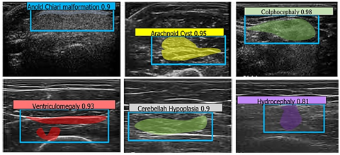
Figure 12 shows the results of the designed multiclass NeuroSegNet model for various Neurological Conditions. Proposed work is a deep learning-based neuro panoptic segmentation object detection approach which processes and diagnoses big sets brain scan images to find neurological abnormalities, achieved an overall accuracy of 98.2%.
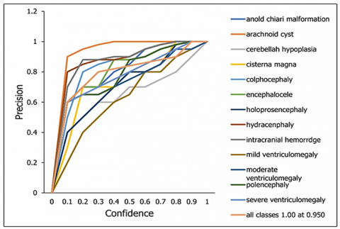
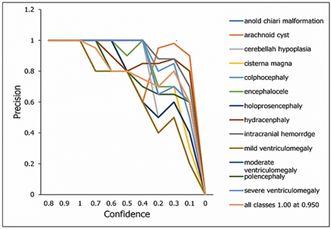
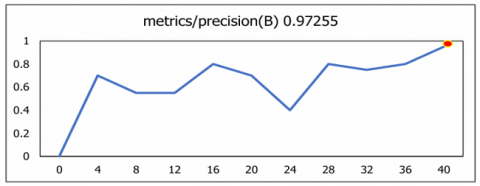
The plotting of the precision-confidence curve depicts the achieved precision value against various confidence thresholds for all classes. It serves as a vital metric showcasing the model's precision at different confidence levels. The proposed model shows high level of precision of 95% as shown in Figure 13. A precision score of 1.00 indicates that the U-NeuroSegNet did not make any false-positive predictions.
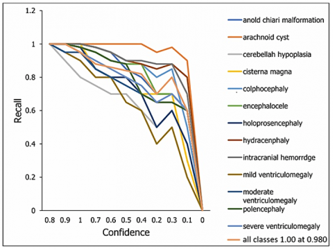
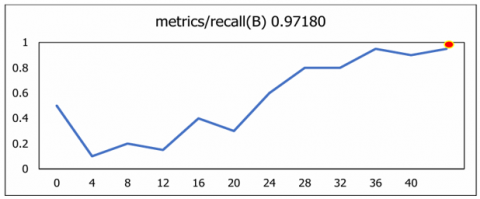
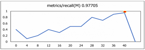
The curve illustrates the recall achieved against several threshold values of confidence. All classes 0.98 at 0.00 means that all classes exhibited recall rate of 98% based on true positives results as the graph-plot represents in Figure 14. The trade-off between recall and precision across a range of confidence thresholds is displayed by the Precision-Recall curve. Every class is showing 0.944 mAP@0.5. Figure 15 illustrates that the proposed U-NeuroSegNet's precision at Intersection over Union (IoU) in ground truth at a 0.5 threshold is 94.4.
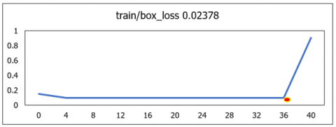
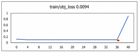
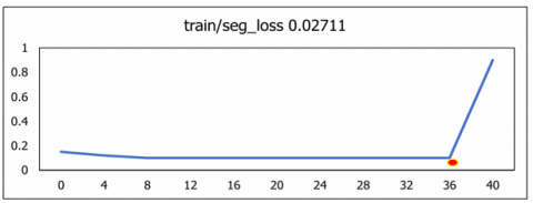
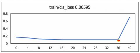
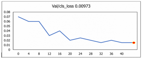
The diagonal value of classes illustrates the correct classification and off diagonal values indicates wrong classification done. The overall classification performance across all classes is 98.2%, as illustrated in Figure 16. To quantify losses in the training data, the metrics Classification_Loss, Object_Loss, Segmentation_loss and Box_loss was used to evaluate the U-NeuroSegNet model. In this model, the performance of the deep NIWatershed algorithm over the training data is found to be optimal. In the proposed deep U-NeuroSegNet model, the training loss over dataset is typically measured after each iteration. The validation loss is measured over fresh, unknown data, while the training loss indicates how well the model performs, or how well it fits the trained data. Figure 17 illustrates very low to negligible loss of the proposed model experienced for all classes.
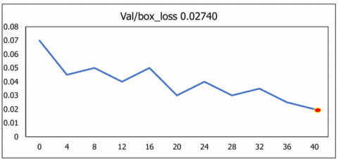
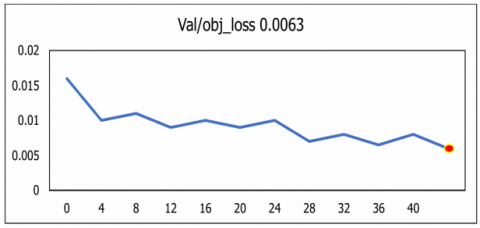
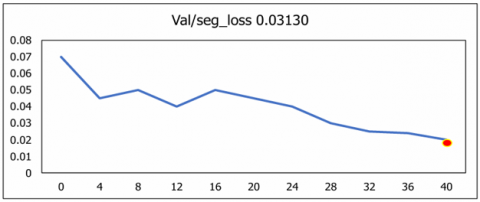
The U-NeuroSegNet model was evaluated using the Mean Average Precision (mAP) metric, which serves as a widely adopted standard for measuring the performance of object detection and segmentation algorithms in computer vision. This metric is particularly effective for benchmarking models in complex segmentation tasks where accurate localization and classification of multiple classes are required. As shown in Figure 18, the evaluation was conducted at an Intersection over Union (IoU) threshold of 0.5, denoted as @mAP 0.5. This threshold provides a meaningful balance between localization precision and overlap tolerance, reflecting the model’s capability to accurately identify and segment target structures across the dataset. The results demonstrate the robustness and high detection accuracy of the U-NeuroSegNet framework in neuroimaging applications.
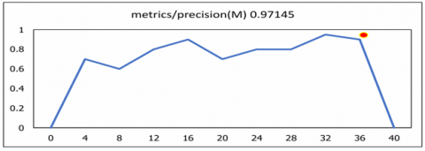
Precision and Recall were further analysed to evaluate the model’s sensitivity and its ability to consistently identify relevant anatomical structures. Collectively, these metrics are summarized in Figure 19. The results demonstrate the robustness and high detection accuracy of the U-NeuroSegNet framework in handling complex neuroimaging data.
The evaluation of the proposed U-NeuroSegNet model across a standardized set of test queries resulted in an impressive mean average precision of 97.3%, as reported in Figure 20. This high mAP score demonstrates the model's capability to consistently and accurately segment and detect neuroanatomical structures, outperforming several existing benchmark models. The consistent performance across various test scenarios highlights the adaptability and precision of U-NeuroSegNet in handling both structured and unstructured image data.
Figure 10. Representation of training batches
Figure 11. Representation of valid prediction batches
Figure 12. Multiclass U-NeuroSegNet prediction for various neurological conditions
Figure 13. Precision-confidence curve of the model over the classes
Figure 14. Recall-confidence curve of the model over the classes
Figure 15. The U-NeuroSegNet model’s precision-recall curve over the classes
Figure 16. Performance across various labels using confusion matrix
Figure 17. Train dataset over loss functions
Figure 18. Validation dataset over loss function
Figure 19. Metrics over recall, precision and mean average precision
Table 6. Performance evaluation of various metrics
|
Metrics/ Authors |
R-CNN |
Mask R- CNN |
MSCA UNet |
3DUNet |
VGG-16 |
U-NEURO SEGNET |
|
Training Image |
1000 |
800 |
1200 |
1500 |
900 |
15000 |
|
Testing Image |
300 |
200 |
400 |
250 |
350 |
500 |
|
Splitting Ratio |
70:30 |
80:20 |
75:25 |
60:40 |
65:35 |
70:30 |
|
Testing Accuracy |
85% |
87% |
84% |
88% |
83% |
94% |
|
Optimizer |
Adam |
SGD |
SGD |
Adam |
Adam |
RMSProp |
|
Algorithm |
VGGNet |
ResNet |
Mobile Net |
LeNet |
Alex Net |
Watershed |
|
Final Layer Activation Method |
Sigmoid |
ReLU |
Tanh |
Sigmoid |
ReLU |
Softmax |
|
Specificity |
0.85 |
0.88 |
0.82 |
0.86 |
0.83 |
0.95 |
|
F1-Score |
0.88 |
0.89 |
0.87 |
0.90 |
0.86 |
0.95 |
|
Sensitivity |
0.90 |
0.92 |
0.88 |
0.91 |
0.89 |
0.94 |
|
Loss |
5% |
4% |
6% |
3% |
5% |
2% |
|
Speed |
30 sec |
25 sec |
35 sec |
40 sec |
28 sec |
20 sec |
|
Evaluation of the Model |
77.81 |
90.11 |
62.74 |
88.52 |
77.98 |
96.81 |
|
Precision |
87 |
89 |
86 |
90 |
85 |
97 |
|
Accuracy |
0.88 |
0.90 |
0.87 |
0.91 |
0.86 |
0.98 |
Figure 20. Performance measures improved by using proposed system
The performance metrics of proposed model includes F-score, sensitivity, precision, accuracy, and testing accuracy, exceed those of all previous works. This indicates the superior capability of proposed model to accurately detect and classify abnormal neurological conditions shown in Table 6. The model evaluation demonstrates a low error rate of only 1.8%, indicating the robustness of our model in minimizing classification errors.
U-NeuroSegNet was designed based on panoptic segmentation to identify abnormal neurological condition using medical images. The developed model was run over big data apache spark GPU based environment. In Spark clusters, the yolo files are placed in its data center folder. This model can identify thirteen types’ neurological conditions. Earlier research works only focused on one class like Arnold Chiari malformation and Ventriculomegaly but in proposed model that can detect hirteen types for neurodegenerative disorders. The system developed is highly efficient and robust, resulting in quicker and more precise identification and segmentation of degenerative neurological anomalies in medical images. By integrating real-time or near-real-time processing capabilities, the system significantly accelerates the diagnostic workflow, allowing healthcare professionals to make informed decisions more swiftly. The work on brain neurological abnormalities classification based on neuro oncology is a powerful tool. The system's high performance in rigorous evaluation and validation studies underscores its reliability and utility in clinical practice. To ensure the system's seamless integration into appropriate clinical workflows and its widespread adoption by healthcare professionals, ongoing efforts to refine and optimize it are vital. By combining technological innovation with practical application, proposed U-NeuroSegNet model stands as a pivotal tool in improving advanced medical imaging procedures and the general standard of neurology care. The potential of proposed model is huge for changing the way brain imaging is used in diagnosing and treating neurological diseases. Future plans include expanding the proposed class offerings to serve as a comprehensive model for diagnosing neurological disorders. In the future there is lot of scope for improvement in model optimization, hardware acceleration, parallel processing and may be employed to further enhance computational speed and efficiency.
[1] Rajaraman, S. (2024). Artificial Intelligence in neuro degenerative diseases: Opportunities and challenges. AI and Neuro-Degenerative Diseases, 1131: 133-153. https://doi.org/10.1007/978-3-031-53148-4_8
[2] Young, A.L., Oxtoby, N.P., Garbarino, S., Fox, N.C., Barkhof, F., Schott, J.M., Alexander, D.C. (2024). Data-driven modelling of neurodegenerative disease progression: Thinking outside the black box. Nature Reviews Neuroscience, 25(2): 111-130. https://doi.org/10.1038/s41583-023-00779-6
[3] Patpatia, S.S. (2024). Harnessing machine learning for early detection and prognosis of Parkinson's Disease: A data-driven revolution in neurodegenerative care. Cambridge Open Engage. https://doi.org/10.33774/coe-2024-zfcw8
[4] Iqbal, M.S., Heyat, M.B.B., Parveen, S., Hayat, M.A.B., Roshanzamir, M., Alizadehsani, R., Akhtar, F., Sayeed, E., Hussain, S., Hussein, H.S., Sawan, M. (2024). Progress and trends in neurological disorders research based on deep learning. Computerized Medical Imaging and Graphics, 116: 102400. https://doi.org/10.1016/j.compmedimag.2024.102400
[5] Dhankhar, S., Mujwar, S., Garg, N., Chauhan, S., Saini, M., Sharma, P., Kumar, S., Sharma, S.K., Kamal, M.A., Rani, N. (2024). Artificial intelligence in the management of neurodegenerative disorders. CNS & Neurological Disorders-Drug Targets-CNS & Neurological Disorders), 23(8): 931-940. https://doi.org/10.2174/0118715273266095231009092603
[6] Ganjizadeh, A., Wei, Y., Erickson, B.J. (2024). From pixels to prognosis: AI-driven insights into neurodegenerative diseases. Medical Research Archives, 12(6): 1-20. https://doi.org/10.18103/mra.v12i6.5512
[7] Li, W., Varatharajah, Y., Dicks, E., Barnard, L., Brinkmann, B.H., Crepeau, D., Worrell, G., Fan, W., Kremers, W., Boeve, B., Botha, H., Gogineni, V., Jones, D.T. (2024). Data-driven retrieval of population-level EEG features and their role in neurodegenerative diseases. Brain Communications, 6(4): fcae227. https://doi.org/10.1093/braincomms/fcae227
[8] Mathur, S., Jaiswal, A. (2024). Demystifying the Role of Artificial Intelligence in Neurodegenerative Diseases. AI and Neuro-Degenerative Diseases. Studies in Computational Intelligence, 1131: 1-33. https://doi.org/10.1007/978-3-031-53148-4_1
[9] Mathur, S., Bhattacharjee, S., Sehgal, S., Shekhar, R. (2024). Role of Artificial Intelligence and Internet of Things in Neurodegenerative Diseases. AI and Neuro-Degenerative Diseases. Studies in Computational Intelligence, 1131: 35-62. https://doi.org/10.1007/978-3-031-53148-4_2
[10] Qadri, Y.A., Ahmad, K., Kim, S.W. (2024). Artificial general intelligence for the detection of neurodegenerative disorders. Sensors, 24(20): 6658. https://doi.org/10.3390/s24206658
[11] Rodriguez, R.V., Kannan, H., Shaikh, K., Bekal, S. (Eds.). (2024). Deep Learning Approaches for Early Diagnosis of Neurodegenerative Diseases. IGI Global. https://doi.org/10.4018/979-8-3693-1281-0
[12] Sharma, A., Kala, S., Kumar, A., Sharma, S., Gupta, G., Jaiswal, V. (2024). Deep learning in genomics, personalized medicine, and neurodevelopmental disorders. Intelligent Data Analytics for Bioinformatics and Biomedical Systems. https://doi.org/10.1002/9781394270910.ch10
[13] Kale, M.B., Wankhede, N.L., Pawar, R.S., Ballal, S., et al. (2024). AI-driven innovations in Alzheimer's disease: integrating early diagnosis, personalized treatment, and prognostic modelling. Ageing Research Reviews, 101: 102497. https://doi.org/10.1016/j.arr.2024.102497
[14] Kaur, S., Kim, R., Javagal, N., Calderon, J., Rodriguez, S., Murugan, N., Bhutia, K.G., Dhingra, K., Verma, S. (2024). Precision medicine with data-driven approaches: A framework for clinical translation. AIJMR-Advanced International Journal of Multidisciplinary Research, 2(5): 1-44. https://doi.org/10.62127/aijmr.2024.v02i05.1077
[15] Liu, L., Sun, S., Kang, W., Wu, S., Lin, L. (2024). A review of neuroimaging-based data-driven approach for Alzheimer’s disease heterogeneity analysis. Reviews in the Neurosciences, 35(2): 121-139. https://doi.org/10.1515/revneuro-2023-0033
[16] Gupta, N.V., Murugan, M.D., Shanbhag, S.J. (2025). AI/ML-driven nanocarriers for the management of neurodegeneration. The Neurodegeneration Revolution, 361-372. https://doi.org/10.1016/B978-0-443-28822-7.00023-4
[17] Shaheen, H., Melnik, R. (2024). Brain network dynamics and multiscale modelling of neurodegenerative disorders: A review. arXiv preprint arXiv:2410.23445. https://doi.org/10.48550/arXiv.2410.23445
[18] Thapliyal, K., Thapliyal, M. (2024). AI enhancing digital communication in neurodegenerative disease treatment. AI and Neuro-Degenerative Diseases. Studies in Computational Intelligence, 1131: 155-170. https://doi.org/10.1007/978-3-031-53148-4_9
[19] Demuth, S., Paris, J., Faddeenkov, I., De Sèze, J., Gourraud, P.A. (2024). Clinical applications of deep learning in neuroinflammatory diseases: A scoping review. Revue Neurologique, 181(3): 135-155. https://doi.org/10.1016/j.neurol.2024.04.004
[20] Gutman, B., Shmilovitch, A.H., Aran, D., Shelly, S. (2024). Twenty-five years of AI in neurology: The journey of predictive medicine and biological breakthroughs. JMIR Neurotechnology, 3(1): e59556. https://doi.org/10.2196/59556
[21] Younes, K., Cobigo, Y., Wolf, A., Kornak, J., Rankin, K.P., Faisal Beg, M., Wang, L., Rosen, H.J. (2024). MRI-based multi-class relevance vector machine classification of neurodegenerative diseases. medRxiv. https://doi.org/10.1101/2024.10.07.24315054
[22] Heming, M., Börsch, A.L., Melnik, S., Gmahl, N., et al. (2024). Atlas of cerebrospinal fluid immune cells across neurological diseases. Annals of Neurology, 97(4): 779-790. https://doi.org/10.1002/ana.27157
[23] MacIver, A., Shaheen, H. (2024). Modelling Alzheimer's protein dynamics: A data-driven integration of stochastic methods, machine learning and connectome insights. arXiv preprint arXiv:2411.02644. https://doi.org/10.48550/arXiv.2411.02644
[24] Zhang, T., Hu, Y., Jiang, W., Fang, L., et al. (2015). Sequencing of allotetraploid cotton (Gossypium hirsutum L. acc. TM-1) provides a resource for fiber improvement. Nature Biotechnology, 33(5): 531-537. https://doi.org/10.1038/nbt.3207
[25] Abrol, V., Gupta, H., Shukla, A. (2024). The Power of Data: Leveraging Machine Learning for Parkinson's Disease Diagnosis. In Intelligent Technologies and Parkinson’s Disease: Prediction and Diagnosis, IGI Global Scientific Publishing. https://doi.org/10.4018/979-8-3693-1115-8.ch001
[26] Raj, M., Singh, V. (2021). Brain tumor detection using hybrid approach of fish school search using SVM. In 2021 IEEE 6th International Conference on Computing, Communication and Automation (ICCCA), Arad, Romania, pp. 561-566. https://doi.org/10.1109/ICCCA52192.2021.9666411
[27] ThamilSelvi, C.P., Vinoth Kumar, S., Asaad, R.R., Palanisamy, P., Rajappan, L.K. (2025). An integrative framework for brain tumor segmentation and classification using neuraclassnet. Intelligent Data Analysis, 29(2): 435-458. https://doi.org/10.3233/IDA-240108
[28] Halagali, P., Nayak, D., Rathnanand, M., Tippavajhala, V.K., Sharma, H., Biswas, D. (2025). Synergizing sustainable green nanotechnology and AI/ML for advanced nanocarriers: A paradigm shift in the treatment of neurodegenerative diseases. The Neurodegeneration Revolution, 373-397. https://doi.org/10.1016/B978-0-443-28822-7.00017-9
[29] Saghafi, S., Sanaei, P. (2024). Dynamic entrainment: A deep learning and data-driven process approach for synchronization in the Hodgkin–Huxley model. Chaos: An Interdisciplinary Journal of Nonlinear Science, 34: 103124. https://doi.org/10.1063/5.0219848
[30] Garbarino, S., Tur, C., Lorenzi, M., Pardini, M., Piana, M., Uccelli, A., Arnold, D.L., Cree, B.A.C., Sormani, M.P., Bovis, F. (2024). A data-driven model of disability progression in progressive multiple sclerosis. Brain Communications, 7(1): fcae434. https://doi.org/10.1093/braincomms/fcae434
[31] Oh, Y., Kim, J.S., Park, G., Kim, H. (2024). Data-driven subtypes of deep gray matter atrophy and dopamine availability in early Parkinson's disease. SSRN 4990496. http://doi.org/10.2139/ssrn.4990496
[32] Ding, J., Dan, T., Wei, Z., Cho, H., Laurienti, P.J., Kim, W.H., Wu, G. (2024). Machine learning on dynamic functional connectivity: Promise, pitfalls, and interpretations. arXiv preprint arXiv:2409.11377. https://doi.org/10.48550/arXiv.2409.11377