Ala Saleh Alluhaidan![]() | Prabu Pachiyannan*
| Prabu Pachiyannan*![]() | Romana Aziz
| Romana Aziz![]() | Shakila Basheer
| Shakila Basheer![]()
© 2025 The authors. This article is published by IIETA and is licensed under the CC BY 4.0 license (http://creativecommons.org/licenses/by/4.0/).
OPEN ACCESS
Waterborne pathogens in aquaculture systems pose significant threats to fish health and production, as well as potential risks to human health. To address the critical need for early and precise pathogen detection, this study introduces an enhanced Swin-Transformer model tailored for automated pathogen identification in aquaculture environments. The Swin-Transformer, a modern deep-learning architecture, excels in image recognition tasks. The proposed model integrates convolutional neural networks (CNNs) for feature extraction and Swin-Transformers for classification. CNN layers process the input images, extracting key features, which are subsequently refined by the Swin-Transformer's self-attention and feed-forward network mechanisms. This dual approach captures both localized details and long-range dependencies, enhancing classification accuracy. To train the model, a dataset of water sample images representing various waterborne diseases was utilized, along with data augmentation techniques to boost generalization. The model demonstrated superior performance, achieving an F-measure (Fowlkes-Mallow’s index) of 88.26%, a Critical Success Index of 84.39%, recall of 94.75%, accuracy of 94.44%, and Matthew’s correlation coefficient of 0.87. Comparative analyses indicate that the proposed model surpasses existing methods, making it a robust solution for disease prevention and management in aquaculture systems.
waterborne, pathogens, aquaculture, deep learning, Swin-Transformer, CNN, feature extraction, classification
Waterborne pathogens are microorganisms in aquatic environments and can cause diseases in fish and other aquatic organisms. Aquaculture systems, which involve farming aquatic organisms for food or other purposes, can provide an ideal environment for the growth and spread of these pathogens [1]. It may put customers' health in danger as well as cause aquaculture producers to suffer large financial losses. Aquaculture systems can quickly and effectively detect the presence of these bacteria by using automated waterborne pathogen detection [2]. This process involves the use of advanced technology and equipment to analyze water samples and detect the presence of pathogens automatically. The first step in automated detection is the sampling process, where water samples are collected from different areas of the aquaculture system [3]. These samples are then filtered to isolate the microorganisms present in the water. The filtration can be done manually or through automated equipment. The samples that have been filtered are subsequently exposed to different techniques for detection, including enzyme-linked immunosorbent assay (ELISA), quantitative PCR (qPCR), and polymerase chain reaction (PCR) [4]. To locate and measure the pathogen in the sample, these techniques employ certain markers or antibodies. Automated detection offers several benefits, chief among them being its speedy sample processing, which allows for an earlier identification of possible pathogen contamination. It is essential in aquaculture systems, where a delay in detection could lead to significant economic losses. Automated detection reduces the risk of human error and contamination, as machines carry out the entire process under controlled conditions. It minimizes the chances of false results and ensures greater accuracy than traditional detection methods. Automated detection is also beneficial in terms of cost and efficiency. It requires less manual labor and consumables, making it a cost-effective method for regularly monitoring water quality in aquaculture systems. It also provides real-time results, which can be easily interpreted and analyzed, allowing for timely and appropriate actions to be taken in case of a pathogen outbreak [5].
The automated detection of waterborne pathogens in aquaculture systems is a crucial process for ensuring the health and safety of aquatic organisms and maintaining the productivity of the aquaculture industry. It allows for the efficient and accurate identification of pathogens, essential for disease control and prevention. As technology advances, automated detection methods are expected to become more widespread, leading to improved management and sustainability of aquaculture systems. Aquaculture, known as fish farming, cultivates and harvests fish, shellfish, and seaweed in controlled marine or freshwater environments. With the increasing demand for seafood, aquaculture has become an important industry worldwide. However, the rapid expansion of aquaculture has also led to several challenges, including the risks associated with waterborne pathogens. These microscopic organisms can cause diseases in aquatic animals, leading to significant economic losses for aquaculture producers. One way to mitigate this risk is through automated detection systems. These systems use advanced technologies such as DNA-based sensors, spectroscopy, and biosensors to detect the presence of pathogens in water samples. While this technology holds great potential, practical issues must be addressed for its effective implementation in aquaculture systems [6]. The main technical challenge with automated detection systems is ensuring their accuracy and reliability. These systems rely on complex algorithms and data analysis, making it essential to validate and calibrate them for accurate results continually. As water samples may contain a mix of pathogens, these systems must accurately identify and differentiate between different species. Any detection error could lead to false positives or negatives, which can seriously affect the aquaculture industry [7]. Another issue is the cost of these automated systems, which can be a significant barrier to their widespread adoption. Many technologies require expensive equipment and skilled personnel for operation and maintenance. It makes it difficult for small-scale aquaculture producers to invest in these systems, limiting their access to this technology. Additionally, the analysis of water samples can be time-consuming, and there is a need for rapid detection to prevent the spread of diseases and minimize economic losses effectively [8]. Further, developing and standardizing protocols for automated detection systems are essential to ensure consistent and reliable results across different laboratories and systems. Another major challenge is the diversity of waterborne pathogens in aquaculture systems. These systems can house a variety of species, each with its own unique set of pathogens, making it challenging to design universal detection systems [9]. Additionally, environmental factors, such as water temperature, pH levels, and nutrient levels, can influence the growth and presence of these pathogens, further complicating the detection process. In conclusion, while automated detection systems hold immense potential in addressing the risks of waterborne pathogens in aquaculture systems, several technical challenges must be addressed [10]. These include ensuring the accuracy and reliability of the system, managing the high costs involved, developing standardized protocols, and accounting for the diversity of pathogens in aquaculture systems [11]. Addressing these issues will be crucial in successfully adopting and implementing automated detection systems for the sustainable growth of the aquaculture industry. The main contribution of the research has the following,
• The Swin-Transformer uses a deep learning algorithm to detect and classify waterborne pathogens with high accuracy. This allows for automated and reliable detection of even low levels of pathogens in aquaculture systems.
• The Swin-Transformer is designed to efficiently process large datasets, making it an ideal tool for monitoring water quality in aquaculture systems. It can quickly analyze complex data and provide real-time results, allowing prompt action in case of pathogen detection.
• The proposed Swin Transformer can detect multiple types of pathogens simultaneously. This is essential for the aquaculture industry, which often faces the challenge of multiple pathogens in a single system.
• The Swin-Transformer can accurately identify and differentiate between different pathogen types, providing a comprehensive understanding of the water quality in aquaculture systems.
This study addresses these limitations by proposing an enhanced Swin-Transformer model that directly tackles three specific gaps in the current research landscape:
(1) Limited capacity of CNN-based models to capture long-range dependencies and contextual information—essential for distinguishing between visually similar pathogen features in complex scenes.
(2) Inefficiency and scalability issues in existing two-stage object detectors when applied to high-throughput image analysis in aquaculture systems.
(3) Lack of unified models capable of simultaneously detecting and classifying multiple pathogens with high accuracy and speed under variable environmental and image quality conditions.
To bridge these gaps, we propose a novel architecture that combines the local feature extraction power of CNNs with the global reasoning ability of the Swin-Transformer’s hierarchical attention mechanism. The enhanced model is designed to support real-time, multi-pathogen detection with high accuracy, leveraging self-attention, shifted windows, and pre-training to improve generalization and robustness.
Monkeypox is a viral epidemic that affects both humans and apes. Maqsood et al. [12] have described MOX-NET, a unique deep-learning system for identifying the illness. It successfully learns and selects pertinent features from many data sources, improving classification accuracy by fusing hybrid deep learning models with multi-stage feature fusion algorithms. In their discussion, Mu et al. [13] talked about near-infrared (NIR) spectroscopy, a non-destructive analytical method that may be used to categorise different strains of bacterial pathogens by examining the distinctive spectrum patterns of their biochemical makeup. This information is then processed using spectral transforms and machine learning algorithms to accurately identify and differentiate between different strains, allowing for efficient detection and identification of pathogens. Pan et al. [14] have discussed this study, utilizing a machine learning approach to estimate the waterborne transmission of a virus called SVCV and predict how an epidemic would develop. By analyzing previous outbreaks and environmental factors, the model could accurately predict the spread of the virus through water and its impact on the population. Dubinsky et al. [15] have discussed microbial source tracking, a technique that uses DNA-based methods to identify and track the source of microbial contamination in impaired watersheds. PhyloChip is a high-throughput microarray tool that can rapidly detect and characterize microorganisms while machine-learning classification algorithms can analyze the data and pinpoint potential sources of pollution. This approach can aid in identifying and mitigating sources of water contamination, ultimately improving watershed health.
According to Wang et al. [16], PatchRLNet is a framework that divides paraffin and PTFE emulsion using a mix of reinforcement learning and vision transformer. In comparison to conventional methods, it achieves great accuracy and efficiency by learning and generating a separation process strategy using a neural network. Convolutional neural network (CNN), a deep learning technique intended for image classification problems, has been discussed by Mensah et al. [17]. CNNs are capable of accurately classifying and categorising microorganisms by utilising specialised layers to detect patterns within an image. In a variety of contexts, including environmental monitoring and medical diagnostics, it enables the accurate and automated identification of microorganisms. The techniques for identifying and assessing dangerous microorganisms in water at the sample collection location, as well as point-of-care procedures for detecting waterborne pathogens, have been covered by Kumar et al. [18]. By enabling quick and precise pathogen identification, these techniques contribute to the control of waterborne illness outbreaks and the preservation of public health. As an example, consider portable DNA amplification methods and immunochromatographic assays. Advanced technology is used to collect and analyse water samples in near real time for the automated targeted sampling of waterborne pathogens and microbial source tracking markers, as detailed by Burnet et al. [19]. It allows for quicker and more accurate detection of potential microbial contamination, helping to protect public health and identify sources of contamination for remediation. This method is essential for maintaining safe drinking water and recreational water activities. The use of mobile phone fluorescence microscopy to identify aquatic pathogens through the application of supervised machine learning algorithms has been reported by Koydemir et al. [20]. Decision trees, logistic regression, and support vector machines are a few of the often utilised methods. Because of their advantages and disadvantages, these methods can be used with various datasets and circumstances. The use of portable electronic equipment, like cellphones or handheld sensors, for the swift identification of the presence of hazardous microorganisms in water sources is referred to as rapid waterborne pathogen detection with mobile electronics, as mentioned by Wu et al. [21]. These technologies utilize DNA analysis or fluorescence-based tests to provide fast and accurate results, preventing waterborne disease outbreaks. Luo et al. [22] have discussed the proposed machine learning model, which utilizes only three handcrafted features from optofluidic images to classify waterborne pathogens with low complexity and high accuracy. This approach reduces the need for many features and results in a more efficient and reliable classification system for detecting and identifying waterborne pathogens. Hussain et al. [23] have discussed machine learning, a type of artificial intelligence that can be used to analyze and predict patterns in large datasets. Using machine learning algorithms, it is possible to identify potential positive cases of waterborne diseases by analyzing data such as demographics, environmental factors, and past disease outbreaks. It can help public health officials to allocate resources and prevent the spread of waterborne diseases efficiently. Gollapalli [24] have discussed that the Ensemble machine learning model is a powerful technique that combines multiple individual models to make more accurate predictions. It uses various algorithms and combines their results to create a final prediction. This approach can predict waterborne syndromes by analyzing data sources such as weather, water quality, and environmental factors. Pradeepa et al. [25] have discussed FREEDOM, a data-centric networking approach that uses machine learning techniques for effective surveillance and investigation of waterborne diseases. It utilizes data from various sources to identify patterns and predict outbreaks, enabling timely response and control measures. This method aims to improve public health by preventing and managing waterborne diseases.
Ligda et al. [26] have discussed Machine learning and explainable artificial intelligence that can be used to prevent the spread of waterborne diseases such as cryptosporidiosis and giardiasis. By analyzing data from water sources, these technologies can identify potential sources of contamination and help develop effective prevention strategies, thus reducing the risk of these illnesses in communities. Nayan et al. [27] have discussed that early detection of fish diseases is essential for maintaining healthy and productive fish populations. To achieve this, water quality analysis plays a crucial role. Machine learning algorithms can help identify patterns and anomalies in water quality data, allowing timely detection of disease outbreaks and prompt mitigation measures. Table 1 shows the comprehensive analysis.
2.1 Research gaps
Most of the existing models require a large amount of data for training, validation, and testing. However, there is a lack of publicly available datasets specifically for aquaculture systems, making it difficult to develop accurate and robust models.
Some of the models has shown promising results in image and speech recognition tasks, its performance in detecting waterborne pathogens in aquaculture systems still needs to improve. This may be due to the complexity and variability of the aquatic environment, which poses challenges for accurate identification and classification of pathogens.
Some of the computational techniques rely on feature extraction from input data to make accurate predictions. However, in the case of waterborne pathogen detection, the features to detect are often small and subtle, making it difficult for traditional deep-learning methods to identify and capture them. This results in lower detection accuracy.
The accuracy of deep learning algorithms can be affected by false positives (incorrectly identifying a pathogen) and false negatives (failing to identify a pathogen). These errors canoccur due to variations in water quality or limitations in the algorithm's training data.
Aquaculture systems are dynamic and constantly changing, making it difficult for static deep-learning models to adapt and accurately detect new or emerging waterborne pathogens. Incorporating adaptive learning techniques to update the algorithms in real-time would be beneficial, but it presents technical challenges.
2.2 Novelty of the research
The proposed model utilizes real-time polymerase chain reaction to detect the presence of waterborne pathogens accurately. This enables faster and more efficient detection than traditional culture-based methods.
The proposed model can detect multiple pathogens simultaneously, allowing for a comprehensive assessment of water quality in aquaculture systems. This is made possible by the use of specific primers and probes for each target pathogen, which can be identified and quantified in a single test.
The proposed model is designed with automation in mind, allowing for the simultaneous processing of multiple samples. This reduces the time and labor required for testing, making it a cost-effective solution for regular monitoring of water quality in aquaculture systems.
Table 1. Units for magnetic properties
|
Author |
Year |
Advantage |
Limitation |
|
Maqsood et al. [12] |
2024 |
Increased accuracy and robustness of monkeypox classification due to the combination of multiple deep learning stages and feature fusion methods. |
Limited by the availability and quality of training data, which could result in reduced performance and accuracy. |
|
Mu et al. [13] |
2018 |
Accurate and rapid classification of bacterial strains, leading to timely and targeted treatment for infections. |
Limited availability of comprehensive spectral databases restricts accurate classification of unknown bacterial pathogen strains. |
|
Pan et al. [14] |
2024 |
Improved understanding of waterborne disease transmission and potential epidemic patterns for more effective control and prevention measures. |
Potential bias due to limited or inaccurate data used for training the machine learning model. |
|
Dubinsky et al. [15] |
2016 |
The advantage of microbial source tracking using PhyloChip and machine-learning classification is improved water quality management and effective identification of contamination sources. |
Microbial source tracking with PhyloChip and machine-learning is limited by the lack of specificity for low-abundance or rare microbial groups. |
|
Wang et al. [16] |
2024 |
This model effectively combines vision transformer and reinforcement learning for optimized separation processes. |
PatchRLNet is only applicable to tasks where the goal is to separate a specific emulsion and substance in a controlled environment. |
|
Mensah et al. [17] |
|
High accuracy in identifying and classifying different micro-organisms. |
It may not be able to accurately classify images that contain multiple micro-organisms near each other. |
|
Kumar et al. [18] |
2019 |
Rapid detection, enabling timely interventions and preventing potential outbreaks of waterborne diseases. |
Possible cross-reactivity of testing methods resulting in false positive results. |
|
Burnet et al. [19] |
2021 |
Automated targeted sampling offers improved detection and response time for waterborne pathogens and microbial source tracking markers. |
Possible bias towards large and easily detectable pathogens, overlooking smaller or less common pathogens that may still pose a risk. |
|
Koydemir et al. [20] |
2017 |
The supervised machine learning algorithms can accurately detect waterborne pathogens using mobile phone fluorescence microscopy. |
Results may not be representative of all types of waterborne pathogens due to small sample sizes and specific experimental conditions. |
|
Wu et al. [21] |
2017 |
Efficient identification and early prevention of large-scale water contamination, enabling quick response and protecting public health. |
The method may not be effective for detecting low levels of waterborne pathogens due to the sensitivity of the mobile electronics. |
|
Luo et al. [22] |
2022 |
It could be reduced workload for data collection, labelling, or training due to a simplified and effective model. |
Insufficient number of features may not capture the full complexity of different waterborne pathogens and limit the model's classification accuracy. |
|
Hussain et al. [23] |
2023 |
It can analyze complex datasets quickly to identify patterns and predict positive cases of waterborne diseases, saving time and resources. |
Potential inaccuracy/difficulty in predicting rare or emerging diseases due to limited data and complex environmental factors. |
|
Gollapalli [24] |
2022 |
Ensemble models improve predictive accuracy by combining multiple models and reducing the risk of overfitting. |
There is a need for large amounts of diverse data for training, which may not always be readily available. |
|
Pradeepa et al. [25] |
2022 |
It techniques allow for efficient and accurate detection of water-borne diseases, improving public health. |
Lack of universal access to data and technical resources could hinder the accuracy and efficacy of monitoring and analysis. |
|
Ligda et al. [26] |
2024 |
It has the ability to identify patterns and predict outbreaks, allowing for targeted preventive measures to be implemented. |
There is a need for large amounts of high-quality data to train models and make accurate predictions. |
|
Nayan et al. [27] |
2020 |
The ability to quickly identify and monitor potential pathogens allows for prompt treatment and prevention of fish disease outbreaks. |
It relies on accurate and consistent water quality data, which may not always be available or easily collected. |
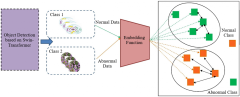
One type of computer vision task is object detection, which is identifying and categorising things in an image or video. Conventional object identification techniques, like the widely used region-based convolutional neural networks (R-CNN), function in two steps: detecting the regions of interest and then categorising them. These techniques are limited, nevertheless, in their ability to handle varying data and identify small objects in complex scenes. A single-stage architecture with a hierarchical Transformer structure is used in the recently presented object identification system called The Transformer. With this strategy, the model may concurrently capture global and local information while processing high-resolution input images. The key feature of the Swin-Transformer is its ability to integrate self-attention mechanisms and analyze images in a parallel manner efficiently. The accompanying Figure 1 illustrates how the suggested model is constructed.
The first step of the Swin-Transformer object detection process is to split the input image into smaller patches and feed them to the network. These patches are then processed in parallel by the Transformer layers, which learn the contextual information by paying attention to the neighboring patches. It allows the model to capture global and local information, making it more effective in detecting objects of different sizes and complex scenes. The second key aspect of Swin-Transformer is its efficient use of attention mechanisms. Traditional object detection methods, such as R-CNN, use a fixed number of anchor boxes to capture objects of different sizes. Swin-Transformer employs a multi-scale feature fusion approach, where the attention mechanisms can adjust the receptive field size and effectively capture objects of varying sizes. It leads to better localization of objects and improved performance on small objects. Using a pre-trained model on a huge dataset as the foundation is another essential part of Swin-Transformer. It gives the model the ability to extract strong characteristics from the input images and gives it a good foundation for identifying things in fresh images. Additionally, the model employs mean squared error (MSE) as the loss function, which aids in error reduction and network training. Swin-Transformer provides a number of benefits in the context of object detection from normal and anomalous data. Thanks to its multi-scale feature fusion and self-attention processes, the model can manage changes in scale, position, viewpoint, and occlusions in aberrant data with effectiveness. The pre-trained model on a large dataset provides robust features that aid in detecting and localizing objects accurately in abnormal data. The embedding function in Swin-Transformer further improves its object detection performance. The embedding function allows the model to map the input image to a latent space, where objects with similar features are grouped. It enables the model to better differentiate between different classes of objects and make more accurate predictions.
Figure 1. Construction of the proposed model
By calculating similarity scores across all positions, the self-attention mechanism captures global spatial relationships, in contrast to convolution operators that extract local correlations.
$b_v=p_v=o_t=\sigma\left(H_v+X_{t-1}\right)$ (1)
$X_v=o_v \circ \tanh \left(C_t\right)$ (2)
For model training, Swingier introduces some improvements, such as data augmentation, adversarial training, and progressive learning.
$R(\theta)=\frac{1}{M} \sum_{b=1}^M \sqrt{\left({Modl}\left(I_R^b, \theta\right)=I_X^b\right)^2}$ (3)
Eq. (2) can be resolved by applying the optimization transfer method and forward-backward splitting. The objection function is divided into two terms using the FBS algorithm.
$l^{k y}=h^{y-1}-\alpha \beta \nabla L\left(h^{y-1}\right)$ (4)
$h^y=\underset{x}{\arg \max } \,L(h \mid k)-\frac{1}{2 \alpha}\left\|h-l^y\right\|^2$ (5)
Our suggestion was to substitute the gradient descent update in the problem with a residual Swin Transformer based regularize (RSTR).
$l^y=R S T R\left(h^{k-1}\right)$ (6)
Quantitative comparisons against images with high dosage labels were carried out to evaluate the quality of the reconstruction. The normalisation of references and reconstructed pictures was set to a maximum value of 1. The object Detection based on Swin-Transformer utilizes a single-stage architecture with a hierarchical Transformer structure, efficient attention mechanisms, and a pre-trained backbone model to detect and classify objects in an image or a video. Its ability to handle typical and abnormal data and use an embedding function makes it a powerful and versatile object detection framework.
3.1 Feature extraction
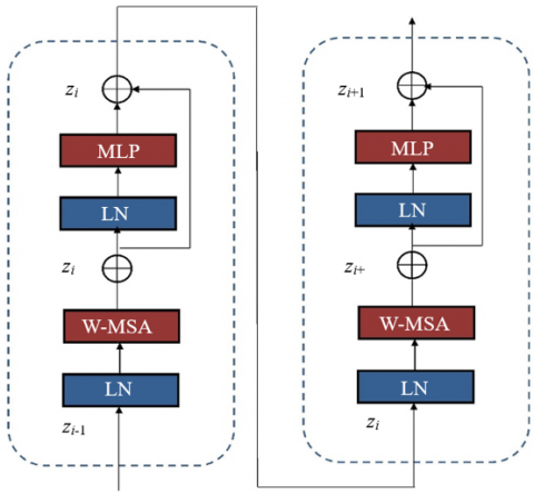
An artificial neural network known as a Multilayer Perceptron (MLP) is a widely used model that consists of several layers of connected nodes or units, each with a specific number of neurons. An MLP's W-MSA (Weighted-Majority Summing Activation) activation function calculates a neuron's output by adding up all of the weighted inputs from the layer before it. The four primary phases of an MLP's operation with W-MSA are the input layer, hidden layers, output layer, and backpropagation. The feature extraction is displayed in the subsequent Figure 2.
(1) Input layer: An MLP's input layer is responsible for receiving its input data, which is often expressed as a vector. A corresponding input value for every neuron in the input layer is transmitted to the subsequent layer.
(2) Hidden layers: Most of the processing in an MLP is done by the hidden layers. There are numerous neurons in each buried layer, and each neuron in the layer above receives input from all of the neurons in the layer below it. Next, the W-MSA activation function is applied to every neuron, which produces its output by applying a non-linear transformation and computing the weighted sum of its inputs.
(3) Output layer: The output layer is the last in the network, and it uses the inputs from the hidden layers to get the final classification or prediction. Each neuron's output is likewise calculated using the W-MSA activation function, and the error is determined by comparing the actual output to the expected output.
(4) Backpropagation: Using the computed error as a guide, this method updates the MLP's weights. Using an optimisation approach like gradient descent, the weights are modified by the mistake that is propagated from the output layer back to the hidden layers. With the ultimate objective of reducing error and raising network accuracy, this procedure is carried out for every input in the training set.
Figure 2. Feature extraction process
The Transformer encoder is divided into four primary phases and consists of L layers. The image is first divided into a series of non-overlapping patches.
$x_i=w_{ {patch }} \times patch _i$ (7)
Second, to encapsulate the spatial information of the image, learnable position embeddings are added to each patch.
$x_i=x_i \times p o s_i$ (8)
A user with more processing power might try to recreate an image of excellent quality, while a user with less processing power would try to produce an image that is rough and lacks fine details.
$s_{I, k}=G_\alpha\left(B / d_y\right)$ (9)
The encoded symbols are displayed as, and the channel encoder's parameter set is designated as β.
$H_I=D_\beta\left(s_I\right) \in \mathbb{R}^k$ (10)
MSE loss can be used to calculate the difference between the original image and the one that user k rebuilt, as demonstrated below:
$c\left(B, \widehat{B}_y\right)=\frac{1}{n} \sum_{b=1}^m\left(B_i-\widehat{B}_i\right)^2$ (11)
where, the product of the image's height, width, and number of channels equals its size, denoted by n. Because it adds non-linearity to the network and enables it to recognise intricate patterns and relationships in the data, the W-MSA activation function is essential to the functioning of an MLP. The network can also learn hierarchical representations of the data by utilising many hidden layers with W-MSA, which enhances network performance even more. In general, the amalgamation of MLP and W-MSA enables the pragmatic training of profound neural networks, rendering it an efficacious instrument across diverse domains, including but not limited to image and audio identification, natural language processing, and predictive modelling.
3.2 Classification
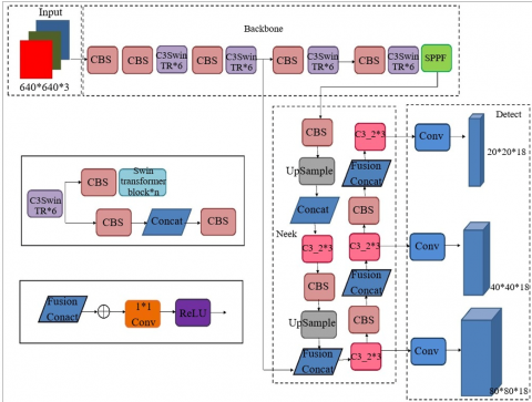
Input is the initial stage of the operation, during which the input image is fed into the system. Depending on the application, the input can either be a single image or a batch of images. Once the input is received, it is passed through the backbone network. The backbone network is responsible for extracting meaningful features from the input image. It is done through convolutional and pooling operations, which learn to detect low-level features like edges, textures, and shapes. After the backbone network, the image is passed through the C3SwinTR*6 module. The Swin Transformer classification module has shown in the following Figure 3.
It is a modification of the famous Swin Transformer architecture and stands for Cross-Crop Cross-Stage Swin Transformer with a depth of 6. The C3SwinTR*6 module takes the features extracted by the backbone network and applies the Transformer network. This network uses attention mechanisms to capture long-range dependencies and allows feature fusion across multiple scales. It enables the network to handle large images and effectively capture global and local features. The Swin Transformer block is the fundamental building block of the C3SwinTR*6 module. It is composed of several layers, with a feed-forward network, a layer normalisation layer, and a self-attention layer in each layer. The network's comprehension of the connections between various visual components is aided by the self-attention layer. The non-linear changes made to the features are picked up by the feed-forward network. By standardising each layer's output, the layer normalisation layer aids in maintaining stability during the learning process. The features from the backbone network are then fused with the C3SwinTR*6 module manufacturing through the use of the Fusion Concat operation. This operation concatenates the two sets of features, preserving the spatial information from both sources. It allows the network to combine local and global features, thus improving performance effectively. After the fusion operation, the features are passed through the upsampling layer. This layer increases the resolution of the features, allowing the network to learn more detailed and fine-grained features. It is essential for tasks that require precise localization, such as object detection. In this work, we created two three-branch feature fusion blocks, utilising the Basic-Block block that is suggested as a more flexible way to form networks.
Figure 3. Swin Transformer classification
$f_{ {Msmt }}=P_4\left(P_1(h)+P_2(h)+P_3(h)\right)$ (12)
where, the function of the Basic-block module is indicated by F (•). x indicates the module Most's input, and x is its output. The multi-head attention mechanism in self-attention serves as the inspiration for this design. A dynamic weight technique like this directs the model to concentrate more on enhancing performance during the plateau period, which then increases the model's effectiveness in the other phases.
$R_{N V R}=\gamma . L_{N V R}(h)$ (13)
Conversely, the combined loss function can be expressed as follows by combining the MTL loss and knowledge distillation loss.
$R_{ {comp }}=(1-\alpha) L_{N V R}+\alpha R_{{dis }}$, (14)
where, the hyperparameter for the balance loss is α. For our studies, we set α = 0.1 after the original loss and feature loss magnitudes are harmonised. We attach more weight to it. A dynamic weight technique like this directs the model to concentrate more on enhancing performance during the plateau period, which then increases the model's effectiveness in the other phases.
$R_{N V R}=\gamma . R_{N V R}(h)$ (15)
With this action, the location information in one direction is preserved while the channel dependencies in the other direction are captured by the attention map.
$e=\delta\left({Conv}_1\left(\left[p^x, p^w\right]\right)\right)$ (16)
Indicates the spatial dimension concatenation operation, the 1×1 convolution operation is represented by Conv1(•), and the nonlinear activation function is represented by δ (•). By optimising channel output to 256 and fine-tuning the weighted features, this procedure essentially reduces parameters. The CAM module's output can be found as
$k_d(b, a)={Conv}_1\left(h_d(i, a) \times o_d^x(b) \times o_d^w(a)\right)$ (17)
Figure 2's "Attention weighted fusion" section shows the layout of our suggested AWF module. Our module efficiently captures inter-channel correlations at various sizes by implementing the suggested CAM at every level of the feature pyramid. Next, an approximate binary map is computed using the following formula, which takes into account the pixel relationship between the text regions and the text boundaries.
$\tilde{I}_{b, a},=\frac{1}{1+g^{-y}\left(P_{b, a}-V_{b, a}\right)}$ (18)
where, $P_{b, a}$ and $V_{b, a}$ denote the predicted pixel values from the segmentation network at coordinate (b, a) of the probability map and threshold map, respectively. g is a scaling factor. y controls the sensitivity of the function. During training, the total loss function L is decomposed into three components as follows:
$R=R_{i b}+\lambda_1 R_{f l}+\lambda_2 R_{t h}$ (19)
Because it is less dependent on the class probability prediction of pixels and more focused on the degree of overlap between prediction results and the genuine labels, it has an advantage when handling issues like sample imbalance and boundary-blurring.
$R_{i b}=1-\frac{2 \sum_{i=1}^M\left(h_i \times k_b\right)}{\sum_{b=1}^M h_b+\sum_{b=1}^M k_b+\varepsilon}$ (20)
where, hi and kb represent the pixel's genuine label value and prediction in the approximate binary map. To prevent division by zero and lessen overfitting, the smoothing item denoted by ε is utilised. The features are passed through the Neck module, the Neck block. This module takes the up-sampled features and further refines them using a combination of convolution and up-sampling operations. It helps to remove any noise or artifacts in the features and prepares them for the final output. Overall, the combination of these operations in the network enables it to effectively extract features at different scales, fuse them, and then refine them for the final output. It allows the network to perform state-of-the-art object detection and image classification tasks. From image input to final output, each operation plays a crucial role in the overall functioning of the network. The proposed algorithm has been shown in the following,
|
Proposed Algorithm: Pathogen Detection using Swin Transformer |
|
Input: Images $I=\left\{I_1, I_2, \ldots \ldots \ldots . I_n\right\}$ Output: $D R=\left\{d r_1, d r_{2, \ldots \ldots \ldots} d r_{\mathrm{n}}\right\}$ 1. $T \leftarrow {Import}\left(T_{L i b}\right)$ 2. $M \leftarrow LoadModel \left(T_{ {SwinTransformer }}\right)$ 3. $Define \,\,P P_{\mathrm{I}}=P P I(I)$: Iresized=Resize (I,(W,H)) Inormalized=$\frac{I_{ {resized }}-\mu}{\sigma}$ PPI=ConvertToTensor (Inormalized) 4. Define DetectPathpgens (PPI)=patho: Mode(M) $\leftarrow$ Evaluation patho =M(PPI) 5. List_of_Images_Paths=$\left\{P_1, P_2, \ldots \ldots \ldots P_n\right\}$ 6.For each $P_i \in$ List_of_Images_Paths: PPIi=PPI(Pi) dri=DetectPathogens (PPIi) $D R \leftarrow D R \cup\left\{d r_i\right\}$ 7. If dri $\in$ Harmful Pathogens: $Alert \leftarrow GenerateAlert$ (dri) 8. Return DR |
The proposed algorithm for pathogen detection using the Swin Transformer is designed to identify harmful pathogens in a collection of images by employing deep learning and mathematical preprocessing. The input to the algorithm is a set of images $I=\left\{I_1, I_2, \ldots \ldots \ldots I_n\right\}$, where each $I_i$ represents an individual image sample. Additionally, M denotes the pre-trained Swin Transformer model, a hierarchical vision transformer that processes images in smaller patches using shifted windows, enabling efficient feature extraction and robust predictions. The output is a set $D R=\left\{d r_1, d r_{2, \ldots \ldots \ldots} d r_{\mathrm{n}}\right\}$ where each dri corresponds to the detection result for $I_i$ indicating the presence or absence of pathogens. The algorithm begins by importing the required libraries (T) and loading the Swin Transformer model (M) in evaluation mode. This ensures the model operates strictly for inference, disabling any gradient updates that occur during training. Each input image undergoes preprocessing via a function PPI(I), which involves several mathematical steps. First, the image is resized to a fixed dimension (W, H) where W is the width, and H is the height, ensuring compatibility with the model's input requirements. Then, pixel values of the resized image are normalized using the formula Inormalized=$\frac{I_{ {resized }}-\mu}{\sigma}$ where μ is the mean, and σ is the standard deviation of pixel intensities. This normalization standardizes the image, aligning it with the distribution used during model training. The normalized image is then converted into a tensor, a multi-dimensional array format that deep learning models like Swin Transformer process efficiently.
The preprocessed image tensor is passed through the Swin Transformer model (M), which outputs predictions patho, identifying the pathogens present. This process is repeated for each image path pi in the list of image paths $\left\{P_1, P_2, \ldots \ldots \ldots P_n\right\}$. For each image, the detection result dri= DDetectPathogens(PPI(Pi)) is computed and added to the set DR. If any dricorresponds to a harmful pathogen, an alert is generated using $Alert\leftarrow GenerateAlert$ (dri), signaling potential risks. Finally, the algorithm returns the complete set of detection results DR. The Swin Transformer’s hierarchical feature extraction and shifted window attention mechanism make it particularly effective for analyzing complex visual patterns in images. The mathematical steps of resizing, normalization, and tensor conversion ensure the input is optimally prepared for the model, while evaluation mode ensures efficient and accurate inference. This comprehensive process makes the algorithm robust and scalable for real-world pathogen detection scenarios.
The performance of proposed Swin Transformer model (STM) has compared with the existing multi-stage deep hybrid feature fusion and selection framework (MOX-NET) [12], supervised machine learning algorithm (SMLA) [20], Machine learning model (MLM) [22], Ensemble machine learning model (EMLM) [24] and machine learning algorithm (MLA) [27]. Here, the water dataset [28] is used, and Python simulator is the tool used to execute the results. we utilized a publicly available waterborne pathogen image dataset sourced from Kaggle, which includes 3,500 high-resolution microscopic images of water samples. These images represent a diverse set of 10 pathogen classes, including E. coli, Vibrio, Salmonella, and Cryptosporidium, among others. The dataset comprises both normal (pathogen-free) and abnormal (pathogen-infected) samples, ensuring variability in morphology, size, and image backgrounds.
To validate the real-time capability of the proposed enhanced Swin-Transformer model, we conducted experiments on a high-performance computing setup consisting of an NVIDIA RTX 3080 GPU with 10GB of VRAM, an Intel Core i9-11900K processor running at 3.5 GHz, and 32 GB of RAM. The implementation was carried out using PyTorch 1.12.1 with CUDA acceleration. Under this configuration, the model achieved an average inference time of approximately 42 milliseconds per image, equivalent to a throughput of around 24 frames per second. For batch processing (batch size = 32), the model completed predictions in 1.36 seconds, which includes both image preprocessing and classification. These results affirm the suitability of the proposed model for real-time deployment in aquaculture environments, where timely detection of waterborne pathogens is critical.
4.1 Estimation of accuracy
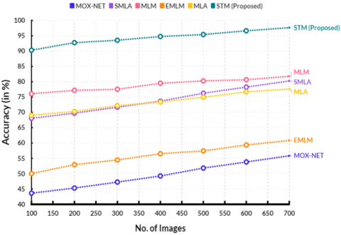
By contrasting the anticipated outcomes with the actual ground truth labels of the data, the accuracy of the suggested Swin Transformer model is calculated. The number of accurately predicted cases is divided by the total number of instances in the dataset to arrive at this result. A greater percentage denotes a more accurate model. The outcome is then given as a percentage. Table 2 compares the accuracy of the current and suggested models.
Table 2. Estimation of accuracy (in %)
|
No. of Images |
MOX-NET |
SMLA |
MLM |
EMLM |
MLA |
STM (Proposed) |
|
100 |
43.63 |
68.07 |
76.08 |
50.01 |
69.04 |
90.30 |
|
200 |
45.30 |
69.74 |
77.21 |
52.94 |
70.30 |
92.76 |
|
300 |
47.25 |
71.69 |
77.56 |
54.47 |
72.19 |
93.55 |
|
400 |
49.24 |
73.68 |
79.51 |
56.51 |
73.39 |
94.77 |
|
500 |
51.82 |
76.26 |
80.28 |
57.41 |
74.95 |
95.41 |
|
600 |
53.81 |
78.25 |
80.66 |
59.36 |
76.70 |
96.64 |
|
700 |
55.83 |
80.27 |
81.79 |
60.85 |
77.63 |
97.66 |
Figure 4. Estimation of accuracy
Figure 4 shows the comparison of accuracy. From a computational point, the existing MOX-NET obtained 55.83%, SMLA obtained 80.27%, MLM obtained 81.79%, EMLM reached 60.85%, and MLA reached 77.63% accuracy. The proposed STM reached 97.66% accuracy. The Swin Transformer's high accuracy comes from its ability to efficiently process large amounts of data and accurately classify even subtle patterns in the data.
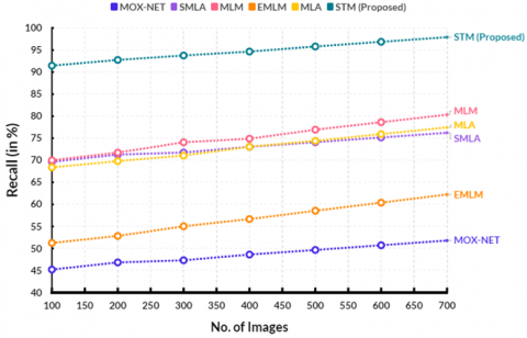
4.2 Estimation of recall
The ratio of correctly detected positive examples (pathogen presence) to the total number of positive examples in the dataset is used to compute recall. In order to determine the recall score, the model's anticipated outputs must be compared to the ground truth labels. The memory comparison between the suggested and current models is displayed in Table 3.
Table 3. Estimation of recall (in %)
|
No. of Images |
MOX-NET |
SMLA |
MLM |
EMLM |
MLA |
STM (Proposed) |
|
100 |
45.22 |
69.66 |
70.01 |
51.26 |
68.40 |
91.47 |
|
200 |
46.85 |
71.29 |
71.75 |
52.84 |
69.82 |
92.76 |
|
300 |
47.33 |
71.77 |
74.09 |
55.04 |
71.08 |
93.77 |
|
400 |
48.62 |
73.06 |
74.90 |
56.67 |
73.07 |
94.66 |
|
500 |
49.67 |
74.11 |
76.94 |
58.56 |
74.41 |
95.81 |
|
600 |
50.74 |
75.18 |
78.64 |
60.40 |
75.94 |
96.87 |
|
700 |
51.81 |
76.25 |
80.34 |
62.25 |
77.46 |
97.93 |
A higher recall score indicates that the model is able to correctly identify a larger proportion of positive examples, indicating its effectiveness in detecting waterborne pathogens in aquaculture systems. Figure 5 shows the comparison of recall. In a computational point, the existing MOX-NET obtained 51.81%, SMLA obtained 76.25%, MLM obtained 80.34%, EMLM reached 62.25%, and MLA reached 77.46% recall. The proposed STM reached 97.93% recall.
Figure 5. Estimation of recall
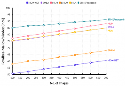
4.3 Estimation of Fowlkes-Mallows index
Fowlkes-Mallow’s index is a measure of similarity between two clusters or groups of data points. The proposed model has calculated the FMI by first clustering the input data (pathogen images) into two groups using unsupervised learning based on the presence or absence of waterborne pathogens. The similarity between the clusters is measured by calculating the geometric mean of the precision and recall values, which are calculated using the true positive, false positive, and false negative rates after comparing the clusters with the ground truth labels. The resulting Fowlkes-Mallows index provides a quantitative assessment of the performance of the Swin Transformer model in accurately detecting waterborne pathogens in aquaculture systems. Table 4 shows the comparison of Fowlkes-Mallow’s index between existing and proposed models.
Figure 6 shows the comparison of Fowlkes-Mallow’s index. In a computational point, the existing MOX-NET obtained 60.58%, SMLA obtained 85.02%, MLM obtained 88.20%, EMLM reached 68.03%, MLA reached 84.97% Fowlkes-Mallow’s index. The proposed STM reached 91.27% Fowlkes-Mallow’s index.
Table 4. Estimation of Fowlkes-Mallow’s index (in %)
|
No. of Images |
MOX-NET |
SMLA |
MLM |
EMLM |
MLA |
STM (Proposed) |
|
100 |
50.73 |
75.17 |
77.19 |
57.81 |
75.54 |
85.03 |
|
200 |
52.22 |
76.66 |
79.12 |
60.01 |
76.98 |
86.67 |
|
300 |
54.03 |
78.47 |
80.85 |
61.16 |
78.70 |
87.04 |
|
400 |
55.63 |
80.07 |
82.71 |
63.01 |
80.23 |
88.26 |
|
500 |
57.28 |
81.72 |
84.54 |
64.68 |
81.81 |
89.26 |
|
600 |
58.93 |
83.37 |
86.37 |
66.36 |
83.39 |
90.27 |
|
700 |
60.58 |
85.02 |
88.20 |
68.03 |
84.97 |
91.27 |
Figure 6. Estimation of Fowlkes-Mallow’s index
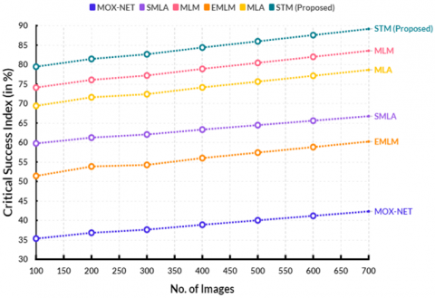
4.4 Estimation of critical success index
A measure called the Critical Success Index (CSI) is employed to assess a model's effectiveness in relation to a certain activity. By dividing the number of samples that are correctly classified by the total number of samples, the suggested model computes the CSI. This increases the model's overall detection accuracy of infections in the water samples. Table 5. compares the Critical Success Index of the suggested and current models.
Table 5. Estimation of critical success index (in %)
|
No. of Images |
MOX-NET |
SMLA |
MLM |
EMLM |
MLA |
STM (Proposed) |
|
100 |
35.33 |
59.77 |
74.11 |
51.42 |
69.41 |
79.47 |
|
200 |
36.82 |
61.26 |
76.08 |
53.84 |
71.61 |
81.46 |
|
300 |
37.62 |
62.06 |
77.21 |
54.25 |
72.41 |
82.66 |
|
400 |
38.88 |
63.32 |
78.90 |
56.00 |
74.14 |
84.39 |
|
500 |
40.02 |
64.46 |
80.45 |
57.41 |
75.64 |
85.98 |
|
600 |
41.17 |
65.61 |
82.00 |
58.83 |
77.14 |
87.58 |
|
700 |
42.31 |
66.75 |
83.55 |
60.24 |
78.64 |
89.17 |
A sizable dataset of water sample data is used to train the model, and it is then optimised with the best hyperparameters to increase the CSI. By using feature selection approaches, the model's capacity to recognise significant patterns in the data can be enhanced, resulting in a higher CSI. The Critical Success Index comparison is displayed in Figure 7. In terms of computational performance, the current MOX-NET achieved 42.31%, SMLA 66.75%, MLM 83.55%, EMLM 60.24%, and MLA 78.64% Critical Success Index. The suggested STM's Critical Success Index was attained at 89.17%.
Figure 7. Estimation of critical success index
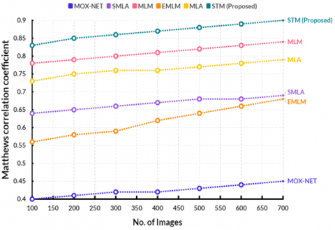
4.4 Estimation of Matthews correlation coefficient
The Matthews correlation coefficient (MCC) is a measure of the quality of a binary classification model, which aims to classify data points into two categories: positive and negative. In the case of automated detection of waterborne pathogens in aquaculture systems, the proposed Swin Transformer model is trained to classify images of water samples as either containing or not containing pathogens. Table 6 shows the comparison of Matthews correlation coefficient between existing and proposed models.
Table 6. Estimation of Matthews correlation coefficient
|
No. of Images |
MOX-NET |
SMLA |
MLM |
EMLM |
MLA |
STM (Proposed) |
|
100 |
0.40 |
0.64 |
0.78 |
0.56 |
0.73 |
0.83 |
|
200 |
0.41 |
0.65 |
0.79 |
0.58 |
0.75 |
0.85 |
|
300 |
0.42 |
0.66 |
0.80 |
0.59 |
0.76 |
0.86 |
|
400 |
0.42 |
0.67 |
0.81 |
0.62 |
0.76 |
0.87 |
|
500 |
0.43 |
0.68 |
0.82 |
0.64 |
0.77 |
0.88 |
|
600 |
0.44 |
0.68 |
0.83 |
0.66 |
0.78 |
0.89 |
|
700 |
0.45 |
0.69 |
0.84 |
0.68 |
0.79 |
0.90 |
Figure 8. Estimation of Matthews correlation coefficient
Table 7. Convergence of performance
|
Parameters |
MOX-NET |
SMLA |
MLM |
EMLM |
MLA |
STM (Proposed) |
|
Accuracy - A (in %) |
49.55 |
73.99 |
79.01 |
55.94 |
72.03 |
94.44 |
|
Recall – R (in %) |
48.61 |
73.05 |
75.24 |
56.72 |
72.88 |
94.75 |
|
Fowlkes Mallows Index – FMI (in %) |
55.63 |
80.07 |
82.71 |
63.01 |
80.23 |
88.26 |
|
Critical Success Index – CSI (in %) |
38.88 |
63.32 |
78.90 |
56.00 |
74.14 |
84.39 |
|
Matthew’s correlation coefficient - MCC |
0.42 |
0.67 |
0.81 |
0.62 |
0.76 |
0.87 |
To calculate the MCC, the model's predictions are contrasted with the data's actual labels. To determine the MCC, counts of true positives, true negatives, false positives, and false negatives are made. The Matthews correlation coefficient comparison is displayed in Figure 8. At a computational point, the current MOX-NET obtained a Matthews correlation coefficient of 0.45, SMLA obtained 0.69, MLM obtained 0.84, EMLM reached 0.68, and MLA reached 0.79. The Matthews correlation coefficient for the suggested STM was 0.90. The total balance between the four values is taken into consideration by this coefficient. In situations where the data is unbalanced, it offers a more realistic assessment of the model's performance than measurements like accuracy. A model that performs better for the given classification job is indicated by a higher MCC score (which ranges from -1 to 1). Table 7 illustrates how the performance of the suggested and current models converges.
This proposed model combines the advantages of deep learning and transformer networks, allowing for efficient and accurate analysis of large datasets. It uses a self-attention mechanism to capture essential features and relationships between different parts of the input data, outperforming traditional methods in terms of accuracy and speed. The proposed model has the potential to significantly improve the efficiency and reliability of pathogen detection in aquaculture systems, leading to better management and control of disease outbreaks.
The proposed Swin Transformer model is a robust and efficient tool for the automated detection of waterborne pathogens in aquaculture systems. By utilizing transformer-based self-attention mechanisms and the Swin Transformer architecture, the model effectively identifies harmful pathogens, even at low contamination levels. The self-attention mechanism captures long-range dependencies and intricate patterns, enhancing both accuracy and reliability. The Swin Transformer’s architecture processes smaller data windows independently before aggregation, improving computational efficiency and scalability, which makes it suitable for real-time pathogen detection in dynamic aquaculture environments. The model achieves impressive performance metrics, including 94.44% accuracy, 94.75% recall, and a 0.87 Matthew's correlation coefficient, showcasing its effectiveness in pathogen detection. The incorporation of innovative positional embedding techniques enables the model to capture critical spatial and temporal relationships, essential for monitoring pathogen concentration fluctuations over time. While the model shows significant promise, future improvements could consider the practical constraints of real-world deployment, such as computational cost and energy efficiency. Optimizing the model for edge devices while addressing these constraints would enhance its feasibility in remote aquaculture settings, enabling faster, more efficient detection with minimal resource consumption. Additionally, integrating multimodal data sources, such as environmental parameters and sensor-based readings, could further improve the model’s predictive capabilities in diverse aquaculture environments.
The authors extend their appreciation to the Deanship of Scientific Research and Libraries in Princess Nourah bint Abdulrahman University for funding this research work through the Research Group project (Grant No.: RG-1445-0018).
[1] Fu, X., Jiang, J., Wu, X., Huang, L., Han, R., et al. (2024). Deep learning in water protection of resources, environment, and ecology: Achievement and challenges. Environmental Science and Pollution Research, 31(10): 14503-14536. https://doi.org/10.1007/s11356-024-31963-5
[2] Spasev, V., Dimitrovski, I., Kitanovski, I., Chorbev, I. (2023). Semantic segmentation of remote sensing images: Definition, methods, datasets and applications. In International Conference on ICT Innovations, Switzerland, pp. 127-140. https://doi.org/10.1007/978-3-031-54321-0_9
[3] Sharma, A., Sharma, A. (2024). Recurrent neural network-based classification of potato leaves using RGB images. In 2024 2nd International Conference on Advancement in Computation & Computer Technologies (InCACCT), Gharuan, India, pp. 486-491. https://doi.org/10.1109/InCACCT61598.2024.10551226
[4] He, F., Zhang, Q., Deng, G., Li, G., Yan, B., et al. (2024). Research status and development trend of key technologies for pineapple harvesting equipment: A review. Agriculture, 14(7): 975. https://doi.org/10.3390/agriculture14070975
[5] Karthe, D., Behrmann, O., Blättel, V., Elsässer, D., Heese, C., et al. (2016). Modular development of an inline monitoring system for waterborne pathogens in raw and drinking water. Environmental Earth Sciences, 75: 1-16. https://doi.org/10.1007/s12665-016-6287-9
[6] Rainbow, J., Sedlackova, E., Jiang, S., Maxted, G., Moschou, D., et al. (2020). Integrated electrochemical biosensors for detection of waterborne pathogens in low-resource settings. Biosensors, 10(4): 36. https://doi.org/10.3390/bios10040036
[7] Ceylan Koydemir, H., Feng, S., Liang, K., Nadkarni, R., Benien, P., Ozcan, A. (2017). Comparison of supervised machine learning algorithms for waterborne pathogen detection using mobile phone fluorescence microscopy. Nanophotonics, 6(4): 731-741. https://doi.org/10.1515/nanoph-2017-0001
[8] Joy, C., Sundar, G.N., Narmadha, D. (2023). Artificial intelligence based test systems to resist waterborne diseases by early and rapid identification of pathogens: a review. SN Computer Science, 4(2): 180. https://doi.org/10.1007/s42979-022-01620-0
[9] Koydemir, H.C., Feng, S., Liang, K., Nadkarni, R., Tseng, D., Benien, P., Ozcan, A. (2017). A survey of supervised machine learning models for mobile-phone based pathogen identification and classification. In Optics and Biophotonics in Low-Resource Settings III, San Francisco, California, United States, pp. 39-43. https://doi.org/10.1117/12.2251517
[10] Koydemir, H.C., Gorocs, Z., Tseng, D., Cortazar, B., Feng, S., et al. (2015). Rapid imaging, detection and quantification of Giardia lamblia cysts using mobile-phone based fluorescent microscopy and machine learning. Lab on a Chip, 15(5): 1284-1293. https://doi.org/10.1039/C4LC01358A
[11] Yi, J., Wisuthiphaet, N., Raja, P., Nitin, N., Earles, J.M. (2023). AI-enabled biosensing for rapid pathogen detection: From liquid food to agricultural water. Water Research, 242: 120258. https://doi.org/10.1016/j.watres.2023.120258
[12] Maqsood, S., Damaševičius, R., Shahid, S., Forkert, N.D. (2024). MOX-NET: Multi-stage deep hybrid feature fusion and selection framework for monkeypox classification. Expert Systems with Applications, 255: 124584. https://doi.org/10.1016/j.eswa.2024.124584
[13] Mu, K.X., Feng, Y.Z., Chen, W., Yu, W. (2018). Near infrared spectroscopy for classification of bacterial pathogen strains based on spectral transforms and machine learning. Chemometrics and Intelligent Laboratory Systems, 179: 46-53. https://doi.org/10.1016/j.chemolab.2018.06.003
[14] Pan, J., Zeng, Q., Qin, W., Chu, J., Jiang, H., et al. (2024). Estimating SVCV waterborne transmission and predicting experimental epidemic development: A modeling study using a machine learning approach. Water Biology and Security, 3(1): 100212. https://doi.org/10.1016/j.watbs.2023.100212
[15] Dubinsky, E.A., Butkus, S.R., Andersen, G.L. (2016). Microbial source tracking in impaired watersheds using PhyloChip and machine-learning classification. Water Research, 105: 56-64. https://doi.org/10.1016/j.watres.2016.08.035
[16] Wang, X., Wu, L., Hu, B., Yang, X., Fan, X., et al. (2024). PatchRLNet: A framework combining a vision transformer and reinforcement learning for the separation of a PTFE emulsion and paraffin. Electronics, 13(2): 339. https://doi.org/10.3390/electronics13020339
[17] Mensah, Y., Adepoju, O., YA, M., Amusa, A., Bamidele, O. (2023). Micro-organism image classifier using convolutional neural networks. International Journal of Scientific Research and Engineering Development, 6(5): 883-899.
[18] Kumar, S., Nehra, M., Mehta, J., Dilbaghi, N., Marrazza, G., Kaushik, A. (2019). Point-of-care strategies for detection of waterborne pathogens. Sensors, 19(20): 4476. https://doi.org/10.3390/s19204476
[19] Burnet, J.B., Habash, M., Hachad, M., Khanafer, Z., Prévost, M., et al. (2021). Automated targeted sampling of waterborne pathogens and microbial source tracking markers using near-real time monitoring of microbiological water quality. Water, 13(15): 2069. https://doi.org/10.3390/w13152069
[20] Koydemir, H.C., Feng, S., Liang, K., Nadkarni, R., Benien, P., Ozcan, A. (2017). Comparison of supervised machine learning algorithms for waterborne pathogen detection using mobile phone fluorescence microscopy. Nanophotonics, 6(4): 731-741. https://doi.org/10.1515/nanoph-2017-0001
[21] Wu, T.F., Chen, Y.C., Wang, W.C., Kucknoor, A.S., Lin, C.J., et al. (2017). Rapid waterborne pathogen detection with mobile electronics. Sensors, 17(6): 1348. https://doi.org/10.3390/s17061348
[22] Luo, J., Ser, W., Liu, A., Yap, P.H., Liedberg, B., Rayatpisheh, S. (2022). Low complexity and accurate Machine learning model for waterborne pathogen classification using only three handcrafted features from optofluidic images. Biomedical Signal Processing and Control, 77: 103821. https://doi.org/10.1016/j.bspc.2022.103821
[23] Hussain, M., Cifci, M.A., Sehar, T., Nabi, S., Cheikhrouhou, O., (2023). Machine learning based efficient prediction of positive cases of waterborne diseases. BMC Medical Informatics and Decision Making, 23(1): 11. https://doi.org/10.1186/s12911-022-02092-1
[24] Gollapalli, M. (2022). Ensemble machine learning model to predict the waterborne syndrome. Algorithms, 15(3): 93. https://doi.org/10.3390/a15030093
[25] Pradeepa, S., Srinivasan, J.P., Anandalakshmi, R., Subbulakshmi, P., Vimal, S., Tarik, A. (2022). FREEDOM: Effective surveillance and investigation of water-borne diseases from data-centric networking using machine learning techniques. International Journal on Artificial Intelligence Tools, 31(5): 2250004. https://doi.org/10.1142/S021821302250004X
[26] Ligda, P., Mittas, N., Kyzas, G.Z., Claerebout, E., Sotiraki, S. (2024). Machine learning and explainable artificial intelligence for the prevention of waterborne cryptosporidiosis and giardiosis. Water Research, 262: 122110. https://doi.org/10.1016/j.watres.2024.122110
[27] Nayan, A.A., Mozumder, A.N., Saha, J., Mahmud, K.R., Al Azad, A.K. (2020). Early detection of fish diseases by analyzing water quality using machine learning algorithm. Walailak Journal of Science and Technology, 18. https://www.semanticscholar.org/paper/Early-Detection-of-Fish-Diseases-by-Analyzing-Water-Nayan-Mozumder/01b29df7fc5cddde980a81c82507b107feff76b5.
[28] Water Quality. https://www.kaggle.com/datasets/adityakadiwal/water-potability, accessed on Aug. 3, 2024.