Arun Inigo Selvaraj*![]() | Tamilselvi Rajendran
| Tamilselvi Rajendran![]() | Parisa Beham Mohammed
| Parisa Beham Mohammed![]()
© 2025 The authors. This article is published by IIETA and is licensed under the CC BY 4.0 license (http://creativecommons.org/licenses/by/4.0/).
OPEN ACCESS
Osteoporosis is a condition in which bones become fragile and prone to fractures. This condition occurs due to reduced Bone Mineral Density (BMD), heredity, smoking, etc. Dual-energy X-ray Absorptiometry (DEXA) images are used for detecting and diagnosing this disease at its earlier stage. Limited generalization across diverse populations, various imaging modalities, and different algorithms were used for extracting the features, but still led to false positives or negatives. This article introduces a Deep Learning-assisted Variance Computation Technique (DL-VCT). In this technique, the learning network is trained using different classes of osteoporosis based on their ranges. The occurrence of any range in the input DEX image is analyzed using the hidden layer processing. In this hidden layer processing, the pixelate features for standard deviation and mean are used for correlating the training class range. The matching ranges are marked under the appropriate osteoporosis classification. The problem of variance detection and suppression is thus handled by the proposed computation technique to improve the precision. The variance from correlation and training is independently extracted to prevent errors. Using this classification, the medical diagnosis is initiated; the variance of BMD is responsible for this classification verified under different learning repetitions. This technique thus improves the detection and classification accuracy of osteoporosis regardless of its stage. From the experimental analysis, it is seen that for the highest classification factor, the proposed technique improves detection accuracy and precision by 8.27% and 13.77% respectively.
Bone Mineral Density (BMD), classification, deep learning, DEXA images, osteoporosis
A prevalent bone condition that often causes disability, especially in the elderly, is osteoporosis. Low Bone Mineral Density (BMD) and the micro-architectural degradation of bone tissue are the direct causes of this disease [1]. Apart from clinical tests, one of the most significant developments is the detection of this disease by X-ray imaging, even if this technique is not widely used in clinical practice [2]. The estimate of BMD in the proximal femur and lumbar spine using DEXA is the standard test for diagnosing osteoporosis. Therapeutic pharmacological therapies for osteoporosis are more successful in the early stages of the illness [3]. Early identification is crucial for preventing osteoporotic fractures-rays can help to detect osteoporosis, an elusive skeletal condition characterized by a decline in bone density and calcium content [4]. The Singh index qualitatively assesses trabecular patterns in the femoral neck to evaluate bone density, with significant correlations observed between cortical thickness, fracture-risk assessments, and femoral neck BMD [5].
Osteoporosis types are primary (postmenopausal/type I and senile/type II) and secondary, with causes like malabsorption, specific medications (e.g., glucocorticoids), and conditions such as hyperparathyroidism [6]. For the diagnosis of osteoporosis risk, DEXA is frequently utilized. DEXA is not often done until symptoms (like a fracture) show up, which might lead to needless exposure of the other organs near the test site [7]. These factors make the use of other widely used modalities essential for an early diagnosis. Computed tomography (CT), for instance, is widely used and comparatively safe. Furthermore, CT can be used to evaluate an individual's risk of osteoporosis [8]. While osteopenia and osteoporosis exhibit texture abnormalities with a decrease in the Hounsfield unit (HU), the typical case has a homogeneous texture [9]. CT features enable assessment of osteoporosis and osteopenia, potentially reducing the social and financial impact of fractures and allowing early treatment. DEXA scans are commonly used to diagnose and monitor osteoporosis and assess body composition [10].
Using deep learning to diagnose osteoporosis from hip radiographs and using clinical data in addition to image mode enhances diagnostic performance. Convolution neural networks (CNN) have a high degree of accuracy when diagnosing osteoporosis from dental panoramic radiographs [11]. The CNN model with fewer parameters was one instance where the ensemble model performed better. Deep learning classification of osteoporosis uses oral panoramic radiographs [12]. In comparison to the image, the inclusion of patient variables enhanced all performance metrics and yielded extra information about significant osteoporosis classifications [13]. Deep learning has enhanced diagnostic accuracy by enabling advanced inference, using clinical data derived solely from dental panoramic X-rays. When combined with a CNN model, it can classify osteoporosis from these radiographs with relatively high accuracy [14]. Furthermore, an ensemble model including patient covariates showed improved classification of osteoporosis. The performance was enhanced using the ensemble model across all CNN models, with fewer parameters proving to be more effective [15]. The contributions are:
• To propose a novel Deep Learning-assisted Variance Computation Technique (DL-VCT) to identify osteoporosis from DEXA images.
• To statistically analyze the BMD through the variance detection in DEXA inputs aided by the deep learning paradigm.
• To analyze the proposed technique’s efficiency through statistical and comparative assessments with different parameters and methods.
The article’s flow is: Section 2 describes the works presented by different authors in the past, with a brief description and the identified problem. Section 3 presents the proposed technique’s description with appropriate equations, diagrams, and descriptions. In Section 4, the experimental and comparative study is presented for and a conclusion is presented in Section 5.
Wang et al. [16] developed a method to estimate lumbar BMD using chest X-rays. This pioneering algorithm shows strong potential for early osteoporosis screening and public health benefits, achieving excellent classification performance. Hwang et al. [17] introduced a Multi-View Computed Tomography Network (MVCNet) to classify osteopenia and osteoporosis using two images from a CT scan. MVCTNet consists of three task layers and two feature extractors, which apply dissimilarity loss to capture distinct features from each image.
Breit et al. [18] introduced an algorithm that computes the spine's attenuation profile, enhancing mean attenuation in patients and aiding in more accurate bone density evaluation. Luo et al. [19] suggested an Osteoporosis Diagnostic Model using Quantitative Ultrasound Radiofrequency Signals with a Multichannel Convolutional Neural Network (MCNN), benchmarked against Dual-energy X-ray Absorptiometry (DEXA). The improved MCNN method achieved a higher area under the receiver operating characteristic curve than the speed of sound, enhancing diagnostic performance. Liu et al. [20] designed a High-precision BMD assessment using an automated, phantom-less QCT system for osteoporosis screening. The primary goal of the method is to verify the precision and accuracy of a single, recently created automatic PLQCT system for the measurement of spinal BMD. Prakash et al. [21] developed 4 x-expert system using multi-model algorithms for early osteoporosis prediction. Machine learning techniques are applied to improve prediction accuracy through various computational processes, enhancing overall prediction performance. Bouzeboudja et al. [22] proposed a Multifractal Analysis for better classification of Osteoporosis. The suggested technique makes it possible to describe the trabecular bone's roughness and local and global regularity in radiographic pictures. The multifractal spectrum is used to uncover alterations in bone microarchitecture brought about by osteoporosis and to extract new texture properties. The proposed method provides excellent promise as an additional tool for osteoporosis diagnosis.
He et al. [23] introduced an Osteoporosis Detection Using Radiomics Based on Lumbar Spine Magnetic Resonance Imaging. The purpose of the model is to investigate a radionics-based lumbar spine magnetic resonance imaging method for osteoporosis detection. The estimated area under the receiver operating characteristic curve was used to assess the classification models' performance. The introduced model increases the detection performance. Keerthika et al. [24] suggested a bio-inspired, intelligent system for osteoporosis prediction and diagnosis. The suggested approach uses an artificial immune system to analyze a classifier and categorize individuals into affected and unaffected groups based on their medical histories. It helps to ascertain the likelihood of this disease in patients. The suggested approach increases the precision and efficiency of the identification process.
Lalitha et al. [25] introduced effective machine learning techniques for the adaptively enhanced Adaboost-based detection of spinal anomalies. Contour-based hybrid median filter with histogram equalization was used to preprocess the data set. The introduced method achieved an accuracy level. Öziç et al. [26] designed a YOLOv5 Deep Learning Model-Based, Fully Automated Osteoporosis Stage Identification on Panoramic Radiographs. The test data that the system was not exposed to previously were examined using the model weights that were acquired. The designed method effectively performs osteoporosis staging and automated localization.
Tang et al. [27] suggested CNN-based approach that primarily consists of two functional modules that analyze the diagnostic 2D CT slice to accomplish qualitative BMD detection. Fang et al. [28] proposed a Multiple-level classification method utilizing a sequential deep-learning algorithm to diagnose osteoporosis and osteopenia. For automated vertebral body segmentation, a fully convolutional neural network known as U-Net was utilized. The proposed model enhances the correlation. Wani and Arora [29] suggested a deep learning strategy that uses transfer learning to categorize various disease stages. The introduced method achieves a better accuracy level. Ramesh and Santhi [30] suggested a Multiple-level classification method utilizing a sequential deep-learning algorithm to diagnose osteoporosis and osteopenia. The suggested approach is used in healthcare datasets related to osteoporosis and osteopenia to improve classification accuracy.
BMD-based osteoporosis detection has been performed with intelligent and bio-inspired methods in the past. In the few other methods discussed above, learning and its image pre-processing features are incorporated. However, the variance in identifying multiple differences between density-reducing and normal regions is tedious due to different pixel distributions and region overlapping. The correlation is therefore required to be intense to identify variance between pixelated and non-pixelated distributions. This single process is lagging in many of the above-mentioned methods, due to which an alternate computation technique using deep learning is introduced in this article.
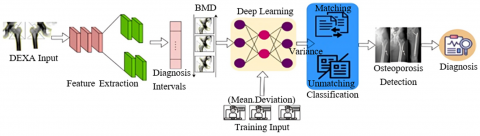
The proposed variance computation technique aims to detect fragile bones prone to fractures; a condition associated with low bone mass that weakens bones and heightens fracture risk, particularly in the spine, wrist, and hip. The method involves using both healthy and affected bone images to train the learning network. The technique is outlined as follows: a DEXA image is inputted, from which features are extracted. The diagnosis intervals are then compared with historical BMD data for the feature-extracted regions. The learning paradigm analyzes the mean and deviation features from the training data to perform classification for matching and non-matching BMD values. This process consolidates the clinical range for diagnosing osteoporosis (Figure 1).
The proposed technique inputs a DEXA image from which feature extraction is performed. The diagnosis intervals are mapped with BMD data from the past for the feature-extracted regions. This value is analyzed by the learning paradigm for the (mean and deviation) features from the training inputs. The classification is performed for the matching and un-matching BMD along with the features. This consolidates the range of clinical osteoporosis values for diagnosis (Figure 1).
Figure 1. Proposed computation technique
3.1 BMD measurement from DEXA images
The DEXA method has been employed from pencil beam to fan beam outputs in high image quality. The primary adult screening is performed mostly with DEXA to reduce the number of individuals at risk of osteoporosis. The DEXA input images observed from the human are processed and then an accurate and precise bone mineral mass is evaluated. Hence, this technique is modeled into two segments such as osteoporosis classification and osteoporosis detection.
3.2 Osteoporosis classification
The equipped detectors are used for screening the tissue and bone from the human body. The different regions this problem will happen. Some regions are the femur, spine, etc. In this input image screening process, the textural patterns require (TP) from the input image is computed as,
$T P=\sum_{d_{i n t l}}^n 1+\frac{o r_{i m a g e}\left(B_D-N_D+\nabla_D\right)}{\sigma}$ (1)
$F_{e x}=\frac{1}{\sqrt{T P}}\left(\frac{O r_{ {image }}}{B_D}-\frac{N_D}{\nabla_D}\right)+2\left(T P-\partial^*\right)$ (2)
where, σ indicates the active detector to record DEXA image for performing pre-processing and segmentation for diagnosis time intervals $d_{intl}$. The variable $O r_{ {image }}$, $B_D$, $N_D$ and $\nabla_D$ are used to show the original image, boundary detection, noise detection, and denoise detection in different screening instances for accurately and easily validating BMD measurement. The variables $F_{e x}$ and $\partial^*$ denote the textural feature extraction and pthe revious healthy bone screened. If $n$ representsthe number of image processing. The uncertainty in detecting osteoporosis is computed as the number of skeletal structure variations observed at different instances is recorded for identifying the break in bone. Some cases of error take place in textural patterns due to reduced bone mineral content or mass, smoking, or heredity are observed at the time of image processing. Therefore, this error affects the textural patterns at any diagnosing interval for which the normalization is evaluated as,
$N(T P)=\frac{\max _{\Delta}}{\left(\frac{\operatorname{Or}_{{image }}}{B_D}-s_{\Delta}\right)^2}$ (3)
And,
$S_{\Delta}=\frac{1}{\sqrt{F_{e x}}}\left(\frac{1}{B_D-1} \sum_{d_{i n t l}=1}^n\left(\frac{T P-\partial^*}{N_D+\nabla_D}\right)^2\right)$ (4)
Eqs. (3) and (4) evaluates the normalization of textural patterns containing the maximum deviation ($\max _{\Delta}$) and standard deviation ($S_{\Delta}$) for accurate variation detection. In this instance, where $S_{\Delta}$ is said to be a normalized measure instead $\max _{\Delta}$ is the uncertain measure evaluated from the given image for which the precise and accurate BMD measurement is made. Based on $F_{e x}$ and $N\left(F_{e x}\right)$, the sequential uncertainty detected from the osteoporosis condition is validated as,
$\begin{gathered}U\left(F_{e x}, N\left(F_{e x}\right)\right)= \sqrt{{\left[\frac{O_{s t e o_c}(R)}{N_D+\nabla_D}\right]_1^2+\left[\frac{O s t e o_c(R)}{N_D+\nabla_D}\right]_2^2+}\ldots+\left[\left(1-\frac{\partial^*}{T P}\right)\max _{\Delta}\right]_{d_{i n t l}}^2}\end{gathered}$ (5)
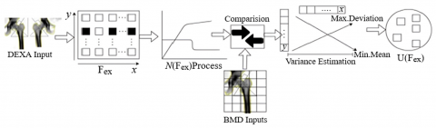
In Eq. (5), the uncertainty sequence is addressed from the instance until the detector is active in screening the tissue and bone from the human body. Where the $Osteo _C(R)$ classes of osteoporosis conditions based on their ranges is trained using hidden layer processing. The uncertainty class for deviation detection is illustrated in Figure 2.
Figure 2. Deviation detection process
The $F_{e x}$ for the input image is normalized for identifying BHD variations across $x$ or $y$. Such variations are normalized for identifying any overlaps are pixel variations. In this process, the BMD variance for $S_{\Delta}$ and $mean$ are computed through comparison. The process relies on variance between $N\left(F_{e x}\right)$ and $F_{e x}$ for the mean and standard deviation. Therefore the $F_{e x}$ that does not belong to $N\left(F_{e x}\right) \forall \partial^*$, the uncertainty is measured. This uncertainty results in a precision decrease (Figure 2). The sequence of uncertainty is validated for detecting and diagnosing the disease at its earlier stage using a DEXA image. In this technique, the ranges are obtained for identifying the osteoporosis condition that must be disseminated in accurate diagnosis intervals to improve the detection. Besides, osteoporosis detection is to be instantaneous in training the learning network using different class regions. Therefore, the occurrence of the different ranges is observed from the input DEXA images used for detecting osteoporosis conditions. Using maximum and standard deviation, the mean $Mean$ is computed as:
$Mean=\max _{\Delta}+S_{\Delta}+{Osteo}_c(R)+N_D+\nabla_D$ (6)
In Eq. (6), the mean is evaluated to extract the features based on ranges. The learning is trained to identify the osteoporosis condition at any instance through hidden layer processing. The first step is to sample the textural patterns and maximum deviation sequence. The correlation of variation is achieved through the expression $\left(1-\frac{\partial^*}{T P}\right) \max _{\Delta}$ is the precise output for osteoporosis classification from the instances. For this purpose, the pixelate features for mean and standard deviation at different diagnosing intervalsare obtained, $Mean$ and $S_{\Delta}$ are serving as the input for correlating the training class range. For this correlation $C_i$ assessment is given as:
${ Mean } \left.=F_{e x}+B_D S_{\Delta}=0\right\} {, }\ as\ the\ first\ variance\ observed$ (7a)
$Mean \left.=N\left(F_{e x}\right) S_{\Delta}=\frac{\max _{\Delta}}{{Osteo}_C(R)}\right\} {, }\ is\ the\ sequence\ of\ variance\ observation$ (7b)
Therefore,
${ Mean }+S_{\Delta}=F_{e x}+B_D,\ is\ the\ first\ training\ input$ (8a)
And,
${ Mean }+S_{\Delta}=N(T P)+\frac{\max _{\Delta}}{{Osteo}_c(R)},\ is\ the\ input\ for\ sequential\ training$ (8b)
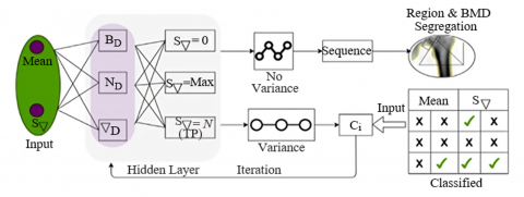
This training initiates from the sequential instances along with the DEXA technology for accurately diagnosing and detecting diseases. The textural patterns and pixelated features are observed from the non-uncertain instance. The correlation of mean and standard deviation is achieved. Hence, the consecutive training of the learning network is accounted for detecting the osteoporosis condition. The occurrence of any range observed in the input DEXA image is analyzed using hidden layer processing. Figure 3 presents the learning process for variance detection.
The mean and $S_{\Delta}$ are the inputs for the learning process along the BMD values. In the joint estimation of $B_D$, $N_D$, and $\Delta_D$, three conditions are identified in the hidden layer (i.e.) $S_{\Delta}=0, S_{\Delta}=\max$ and $S_{\Delta}=N(T P)$. The first two conditions are optimal for $F_{e x}\left[\right.$with $\left.N\left(F_{e x}\right)\right]$ and BMD inputs. Contrarily, $S_{\Delta}=N(T P)$ is exclusive to the variance identified. This generates sequential and variation outputs as in Eqs. (7b) and (8a). Among these, the mean $N\left(F_{e x}\right)$ is the training (Variance) input for $\nabla_D$. The S=0 sequence segregation is the conventional training input for $B_B$. Here, $N_D$ does not require any such iterated training inputs as the variance between the BMD values is identified at any instance (Figure 3).
Figure 3. Learning process for variance detection
The learning network is configured with one input layer, followed by a hidden layer and an output layer. The input layer is assigned the mean and $N_{\nabla}$ neurons for the features extracted. Therefore, these neurons are variable based on the number of maximum and minimum considerations of $B_D$, $N_D$, and $\nabla_D$. The variance between these minimum and maximum values, referencing the difference as 0 is considered for analysis. The detection of zero and non-zero variance is used to segregate the features (representing the regions) and the $C_i$ estimation. This estimation in the hidden layer is eased by the maximum mean and $s_{\nabla}$ classification changes. Thus, the classification is conjoined with the hidden layer output to maximize the variance detection precision from the initiated hidden layer inputs. The process of DL-VCT-based osteoporosis detection and classification requires BMD measurement at different diagnosis intervals through the detector. The osteoporosis conditions are addressed based on matching and un-matching range classification using DL-VCT, depending on the maximum deviation standard deviation and uncertainty function. The noise is initially filtered in the given input image. If matching range $x$ and unmatched rangey raise and fall concerning $d_{i n t l}$ and then x∈(0, ∞) and y∈(-∞, 0) is satisfied based on their range. From the instance, the matching and un-matching range is identified and segregated using correlation output. Based onx andy range at any diagnosis interval $\left(n \times d_{i n t l}\right)$.
As represented in the first and consecutive instance, the hidden layer processing used for the training $\left\{F_{e x}, S_{\Delta}\right.$, Mean$\}$ is performed. In the first instance, the pixelate features and standard deviation are defined as in the above equation. Hence, the BMD measurement with $TP$ is retained with maximum uncertainty. In particular, based on features and diagnosis intervals in the given input DEXA image is analyzed to satisfy either the matching or un-matching range. This is because the Mean and $S_{\Delta}$ are marked using matching ranges under the accurate osteoporosis classification, such that the probability of occurrence is identified from the instance. In this technique, the osteoporosis condition is expressed as $Osteo _c>\frac{ { Mean }}{S_{\Delta}}$ or $Osteo_c \leq \frac{{ Mean }}{S_{\Delta}}$ is evaluated. Using Eq. (9), the $Osteo_c$ and ranges of $Mean$ and $S_{\Delta}$ is mapping to partial output $po$ is given as
$Osteo_c=1-\frac{\rho_{\max \Delta}}{\rho_{S_{\Lambda}}}$ (9)
And,
$\begin{aligned} & S_{\Delta}\left(F_{e x}\right) \ { maps\ to }\ R, { if } \ { Osteo }{ }_c>\frac{ { Mean }}{S_{\Delta}} { else, } \\ & \left.S_{\Delta}\left(F_{e x}\right)\ { maps\ to\ Mean\ or }\ S_{\Delta}, { if } \ { Osteo }_c \leq \frac{{ Mean }}{S_{\Delta}}\right\}\end{aligned}$ (10)
The variables $\rho_{ {max } \Delta}$ and $\rho_{S_{\Delta}}$ shows the probability of maximum and standard deviation from the least possible instance. Now, the hidden layer processing for the conditions $Osteo_c>\frac{{ Mean }}{S_{\Delta}}$ and $Osteo_c \leq \frac{{ Mean }}{S_{\Delta}}$ is expressed as in Eqs. (11) and (12).
$\begin{gathered}H L_1=N\left(F_{ex}\right)_1 H L_2=N\left(F_{e x}\right)_2-\left(\frac{ {Mean}}{S_{\Delta}}\right)_1- \left(\frac{{Osteo}_c(R)}{N_D+\nabla_D}\right)_1 H L_3=N\left(F_{e x}\right)_3-\left(\frac{{Mean}}{S_{\Delta}}\right)_2- \\ \left(\frac{{Osteo}_c(R)}{N_D+\nabla_D}\right)_2 \vdots\ H L_n=N\left(F_{e x}\right)_n-\left(\frac{{Mean}}{S_{\Delta}}\right)_{n-1}-\left.\left(\frac{{Osteo}_c(R)}{N_D+\nabla_D}\right)_{n-1}\right\},\ for\ the\ n\ instances \end{gathered}$ (11)
Such that,
$\begin{gathered}H L_1=F_{e x_1}-S_{\Delta}\left(\frac{x}{y}\right)_1 H L_2=F_{e x_2}-S_{\Delta}\left(\frac{x}{y}\right)_2-\left(\frac{O {steo}_c*R}{N_D+\nabla_D}\right)_1 H L_3=F_{e x_3}-S_{\Delta}\left(\frac{x}{y}\right)_3-\left(\frac{O \text { steo }_c * R}{N_D+\nabla_D}\right)_2 \vdots H L_n \\ \left.=F_{e x_n}-S_{\Delta}\left(\frac{x}{y}\right)_n-\left(\frac{O { steo }_c * R}{N_D+\nabla_D}\right)_{n-1}\right\}, {for\ the}\ n \ {instances}\end{gathered}$ (12)
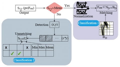
The hidden layer processing outputs are obtained n instances, where the normalization of extracted features from the input DEXA image is analyzed, and the textural patterns and pixelate features are considered factors for determining the classification output. The classification process is illustrated in Figure 4.
Figure 4. Classification of matching and un-matching $F_{ex}$
Classification 1 above describes the matching and Classification 2 describes the un-matching ranges. The $S_{\nabla}<mean$ identifies the precise (x,y) for R segregation. This requires an uncertainty case that elevates $B_D$ and the actual clinical range. Therefore, the chance of unmatching is high due to the actual clinical range [31]. Therefore, the chances of un-matching are high, due to which the iterations are pursued for $N\left(F_{e x}\right)$. The first classification relies on $N_D \pm B_D \forall F_{e x}$ under BMD inputs. This classification achieves high matching post the normalization to satisfy $S_{\Delta}> Mean$ (Figure 4). Based on the range occurrence, the uncertainty function as in Eqs. (7a), (7b), (8a), and (8b) are analyzed and verified for their osteoporosis detection for the conditions of $Osteo_c>\frac{ { Mean }}{S_{\Delta}}$ and $Osteo _c \leq \frac{{ Mean }}{S_{\Delta}}$ using the following evaluations. The osteoporosis classification and detection is performed under various learning repetitions helps to improve the precision and accuracy of this disease detection regardless of its stage [32].
4.1 Radiographic absorptiometry
The radiograph input image is processed, the bone and reference wedge are validated to find the bone density. The advantages of this technique are easiness, low cost, and rapidity in every use in the medical field. The proposed technique is statistically evaluated using the data [33]. This data provides a cumulative mean of BMD values of 564 participants using the screening process. The patients above 50 years of age are considered in this data collection, in which 359 are male and 205 are female. The images are obtained from a dual energy X-ray absorptiometry (DEXA) machine operating two peak X-ray beams: 30-50 keV and 70 keV for BMD measurement. This imaging is used to compute T and Z scores from which the precise bone density is estimated. The radiation dose between 1 and 50 $\mu$Sv is used for measuring the Z and T values. Based on the observed outcomes, the BMD with variance is presented in Table 1. This deviation is used as a T-score to validate the bone density; the range between -1 and 1 refers to a normal mass, -1 to -2.5 indicates lesser bone mass, and above -2.5 refers to the osteoporosis problem. Based on the deviation observed, the classification is presented in the following Table 1 and Table 2.
Table 1. BMD values with the variance identified using the proposed method
|
Type |
Region |
Max. Deviation |
Variance |
Classification |
|
Lumbar spine |
L1 |
0.905 |
$\pm$0.04 |
Normal |
|
L2 |
0.811 |
$\pm$0.01 |
Normal |
|
|
L3 |
0.655 |
$\pm$0.02 |
Normal |
|
|
L4 |
0.729 |
$\pm$0.09 |
Normal |
|
|
L2 |
-0.19 |
$\pm$0.07 |
Low Mass |
|
|
L3 |
0.04 |
$\pm$0.07 |
Normal |
|
|
L4 |
-0.17 |
$\pm$0.11 |
Osteoporosis |
|
|
L3 |
-0.1 |
$\pm$0.06 |
Low Mass |
|
|
L4 |
0.09 |
$\pm$0.03 |
Normal |
|
|
L4 |
0.93 |
$\pm$0.08 |
Normal |
Table 2. Variance occurrence and its chances for different lumbar regions
|
Type |
Region |
Classification Factor |
Occurrence (%) |
Chances |
|
Lumbar Spine |
L1 |
0.2 |
31.90 |
5.25 |
|
0.4 |
26.44 |
3.51 |
||
|
0.6 |
13.96 |
6.60 |
||
|
0.8 |
15.48 |
4.95 |
||
|
1 |
9.83 |
2.53 |
||
|
L2 |
0.2 |
17.82 |
8.30 |
|
|
0.4 |
14.34 |
4.29 |
||
|
0.6 |
28.32 |
7.83 |
||
|
0.8 |
14.47 |
6.67 |
||
|
1 |
29.24 |
8.42 |
||
|
L3 |
0.2 |
20.82 |
2.68 |
|
|
0.4 |
24.83 |
7.76 |
||
|
0.6 |
24.11 |
7.16 |
||
|
0.8 |
22.66 |
5.05 |
||
|
1 |
12.38 |
7.28 |
||
|
L4 |
0.2 |
38.07 |
4.50 |
|
|
0.4 |
27.51 |
4.28 |
||
|
0.6 |
24.55 |
8.57 |
||
|
0.8 |
8.30 |
5.97 |
||
|
1 |
29.45 |
5.74 |
The chances of variance occurrence for different classification ranges for 4 regions are tabulated above. The variance occurrence ratio is estimated by accounting the $Osteo_c>\frac{{ Mean }}{S_{\Lambda}}$ condition across $(x, y) \in R$. Based on the $S_{\Delta}\left(F_{ex}\right)$, the iteration for the consecutive $Mean$ is defined such that $U\left(F_{e x}, N\left(F_{e x}\right)\right)$ is analyzed for multiple $\partial^*$. In this case, as the classification factor increases, the chances based on occurrence are detected with better precision. Yet another consideration is the feature extraction rate based on the noise pixels and image quality, for which the $N_D \pm B_D \forall F_{e x}$ is used to compute its impact on the variances. Therefore, the acquisition parameters, including the device operational frequency and image quality, are accounted for to improve the computation of variation occurrence and its chances (Table 2). Following the above, the computation cost for the training process based on the iterations and classification factors is tabulated in Table 3.
Table 3. Computation cost for training based on iterations and classification
|
Region |
Classification Rate |
Computation Cost |
Iteration |
Computation Cost |
|
L1 |
0.2 |
0.23 |
400 |
0.21 |
|
0.4 |
0.19 |
600 |
0.22 |
|
|
0.6 |
0.58 |
800 |
0.37 |
|
|
0.8 |
0.15 |
1000 |
0.38 |
|
|
1 |
0.60 |
1200 |
0.38 |
|
|
L2 |
0.2 |
0.31 |
400 |
0.35 |
|
0.4 |
0.47 |
600 |
0.34 |
|
|
0.6 |
0.19 |
800 |
0.49 |
|
|
0.8 |
0.58 |
1000 |
0.35 |
|
|
1 |
0.14 |
1200 |
0.35 |
|
|
L3 |
0.2 |
0.43 |
400 |
0.60 |
|
0.4 |
0.20 |
600 |
0.21 |
|
|
0.6 |
0.14 |
800 |
0.59 |
|
|
0.8 |
0.31 |
1000 |
0.41 |
|
|
1 |
0.24 |
1200 |
0.41 |
|
|
L4 |
0.2 |
0.60 |
400 |
0.35 |
|
0.4 |
0.33 |
600 |
0.35 |
|
|
0.6 |
0.54 |
800 |
0.29 |
|
|
0.8 |
0.48 |
1000 |
0.29 |
|
|
1 |
0.24 |
1200 |
0.29 |
The computation cost for the different classification and iterations is presented in Table 3 above. The computation based on recurrent training intervals, the network training rate, drop, and halting rates is computed. For the varying intervals, the need for classification precision is high, for which $\left(T P-\partial^*\right)$ is the computation causing factor. Therefore, new feature extraction and processing until $B_D$ and $N_D$ are classified to prolong the training drop rate. This requires an additional computation cost to reduce $U\left(F_{e x}, N\left(F_{e x}\right)\right)$ using the first and sequential variance observed. Therefore, the computation cost is retained in the next iteration, or the classification rate (high) confines the uncertainty. These two computations for uncertainty reduction control the cost for further classification.
4.2 Experimental analysis
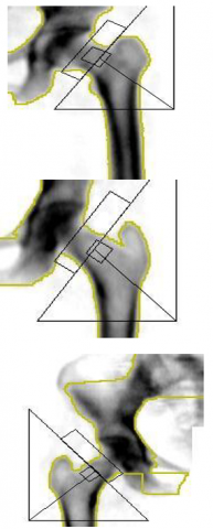
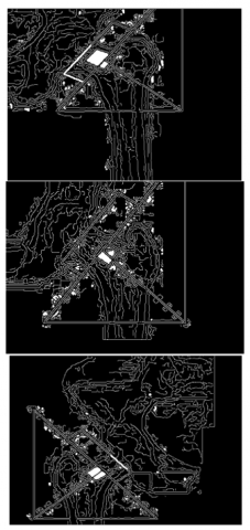
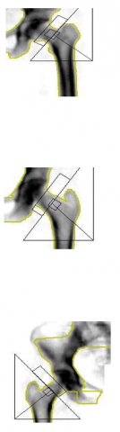
The experimental analysis is performed using the dataset [32] that provides 180 osteoporosis images for testing and 372 images for training. The average run-time is 198.1s with continuous 3 epochs. In this experimental analysis, 2-sample results using MATLAB are presented in Figures 5-6. The dataset contains both normal and osteoporosis images for testing and training; therefore, in the training phase, an imbalance occurs due to feature extraction rates and variance estimation between these two kinds of images. To mitigate this imbalance, the post-extraction is followed by the normalization process before the sequence classification. If the sequence classification shows up difference, then imbalances are found relating to the training input type. In the tables below, the matching and detected regions are highlighted.
(a) Input samples
(b) Variance region
(c) Normalized output
(d) Matching
Figure 5. Osteoporosis region matching output for input samples
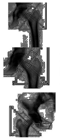
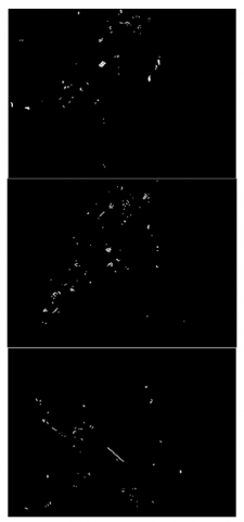
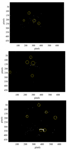
(a) Sample
(b) Un-matching
(c) Classified
Figure 6. Osteoporosis region detected output from input samples
4.3 Comparative analysis
The comparative analysis is discussed using metrics such as detection accuracy, classification accuracy, precision, classification time, and variance. In this analysis, the classification factor, ranging from 0.1 to 1, and the considered methods (MCNN [19], MLC-SDL [30], and MCVTNet [17]) are accounted for.
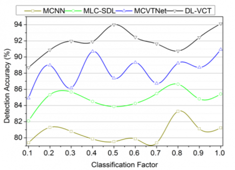
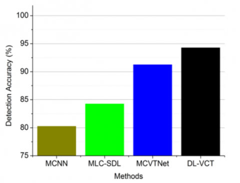
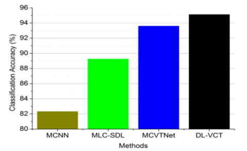
The proposed technique achieves a high bone fracture detection rate using hidden layer processing to identify BMD drops at various diagnosis intervals (Figures 7(a) and 7(b)). It minimizes variance and classification time by maintaining standard deviation and mean consistency during DEXA image processing and segmentation. The DL-VCT method mitigates BMD reduction, with $F_{e x}$ and $\partial^*$ minimizing variation in consecutive instances. The learning network evaluates bone mass, quality, and BMD, using extracted features to determine disease likelihood. Pixilated feature correlation speeds up the process and failed correlations train subsequent inputs to enhance accuracy (Figure 7(c)).
(a) Classification factor
(b) Methods
(c) Classification accuracy
Figure 7. Detection and classification accuracy comparisons
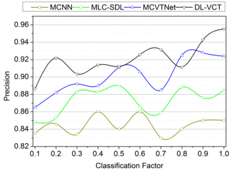
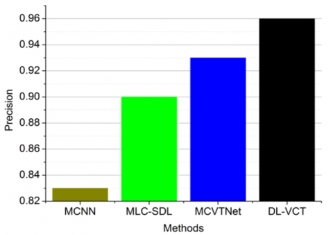
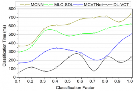
In Figure 8, this article sequentially identifies osteoporosis by classifying matching and non-matching ranges observed in input DEXA images using DL-VCT. The proposed technique achieves high precision in classification and detection through multiple learning repetitions. This proposed technique analyzes textural patterns to identify bone structure breaks. This method enhances disease detection and classification accuracy, allowing for early-stage diagnosis with less classification time using DEXA images and DL-VCT.
Figure 8. Precision and classification time comparisons
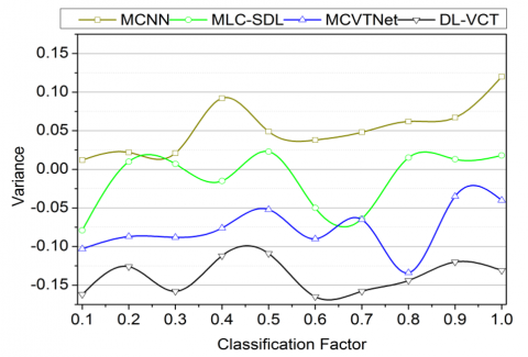
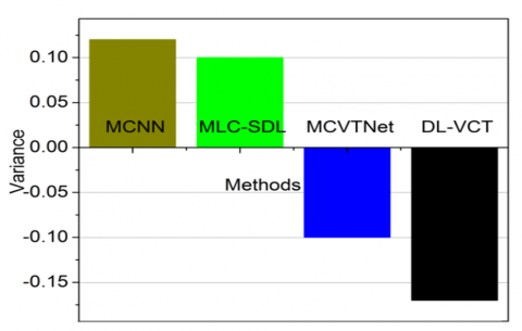
The proposed DL-VC technique detects errors and variance across various diagnosis intervals to maximize detection accuracy and precision for osteoporosis classification. The learning process is trained to identify osteoporosis using hidden layer processing and the proposed method. Textural pattern variations and maximum deviations are analyzed during diagnosis. The correlation between deviation and mean is expressed as $\left(1-\frac{\partial^*}{T P}\right) \max _{\Delta}$ providing precise output for osteoporosis classification. Range occurrences are verified in the input DEXA images to ensure correct classification. Hidden layer processing identifies variance to improve accuracy. The correlation of mean and standard deviation further enhances detection and classification. As shown in Figures 9(a) and 9(b), the DL-VCT reduces variance and improves osteoporosis condition identification. In Table 4, the p-values based on comparative analysis are presented.
(a) Classification factor
(b) Methods
Figure 9. Variance comparisons for (a) Classification factor (b) Methods
Table 4. p-Values Tabulation
|
Classification Rate |
MCNN |
MLC-SDL |
MCVTNet |
Proposed Methodology DL-VCT |
|
0.1 |
0.37 |
0.53 |
0.66 |
0.64 |
|
0.2 |
0.49 |
0.57 |
0.70 |
0.81 |
|
0.3 |
0.44 |
0.61 |
0.46 |
0.74 |
|
0.4 |
0.52 |
0.53 |
0.41 |
0.72 |
|
0.5 |
0.26 |
0.32 |
0.69 |
0.94 |
|
0.6 |
0.57 |
0.57 |
0.71 |
0.85 |
|
0.7 |
0.28 |
0.53 |
0.60 |
0.81 |
|
0.8 |
0.57 |
0.63 |
0.77 |
0.82 |
|
0.9 |
0.26 |
0.53 |
0.48 |
0.71 |
|
1 |
0.63 |
0.75 |
0.87 |
0.95 |
The p-values are tabulated based on the classification rate in Table 4. The p-values are the prime outputs for the classification described in Eqs. (7) and (8). Based on the sequence for classification, the $Mean$ is estimated to improve the feature extraction and normalization. If these two processes are successful, then the variance is estimated with less uncertainty. In the existing methods, the uncertainty mitigation is less due to new feature replacement, based on which the computations for classification are made. Therefore, for the maximum classification rate, the proposed method using the learning network achieves better convergence in precision. The comparative analysis results are summarized in Tables 5 and 6 for the classification factor and methods.
Table 5. Comparative analysis summary for classification factor
|
Metrics |
MCNN |
MLC-SDL |
MCVTNet |
Proposed Methodology DL-VCT |
|
Detection Accuracy (%) |
81.23 |
85.42 |
90.93 |
94.12 |
|
Precision |
0.85 |
0.88 |
0.924 |
0.95 |
|
Classification Time (ms) |
745.79 |
625.42 |
502.52 |
236.94 |
|
Variance |
0.12 |
0.018 |
-0.04 |
-0.13 |
Table 6. Comparative analysis summary for methods
|
Methods |
Metrics |
||||
|
Detection Accuracy (%) |
Classification Accuracy (%) |
Precision |
Classification Time (ms) |
Variance |
|
|
MCNN |
80.26 |
82.32 |
0.83 |
754.1 |
0.12 |
|
MLC-SDL |
84.25 |
89.25 |
0.9 |
457.0 |
0.1 |
|
MCVTNet |
91.25 |
93.6 |
0.93 |
247.1 |
59.52 |
|
Proposed Method (DL-VCT) |
94.263 |
95.12 |
0.96 |
59.52 |
-0.17 |
The proposed technique improves detection accuracy and precision by 8.27% and 13.77% respectively. The proposed technique reduces classification time and variance by 10.34% and 8.37% respectively. These values are précised from the existing method's cumulative sum tallied to the proposed technique mathematically. Besides, the values are presented as the outcome of the final value of the proposed technique.
The proposed technique improves detection accuracy, classification accuracy, and precision by 9.01%, 13.46%, and 14.67% respectively. The proposed technique reduces classification time and variance by 14.63% and 7% respectively. Similar to the comparative analysis results in the previous table, these values are mathematically formulated.
In this article, the DL-VCT to identify osteoporosis using DEXA inputs is introduced and discussed. The BMD variance under various intervals through statistical and image observations are jointly handled using this technique. The input is preprocessed using textural features for BMD and BMD drops at regular intervals. In particular, the mean and standard deviation for the variance assessment are used for identifying osteoporosis classification from training input correlations. Depending on the variance, the matching and un-matching classifications are performed to detect osteoporosis conditions. This complete process is aided by deep learning using its hidden layers for occurrence and correlation. The training is revived using pixel-based features and matching BMD observations with fewer variances. This ideal case is set as the training factor to identify osteoporosis from the input image using different repetitions. From the experimental and comparative analysis, it is seen that the proposed technique improves detection accuracy and precision by 8.27% and 13.77% respectively. This technique also faces the problem of convergence in correlation due to statistical and image differences. Such a problem results in less precision for immediate BMD variances under irregular observation intervals. Therefore, future work is likely to rely on pre-classification-dependent processing from the feature extraction category. Such an option would reduce the difference between actual and observed variance to detect osteoporosis.
[1] Xue, L., Qin, G., Chang, S., Luo, C., Hou, Y., Xia, Z., Yang, K. (2023). Osteoporosis prediction in lumbar spine X-ray images using the multi-scale weighted fusion contextual transformer network. Artificial Intelligence in Medicine, 143: 102639. https://doi.org/10.1016/j.artmed.2023.102639
[2] Mebarkia, M., Meraoumia, A., Houam, L., Khemaissia, S. (2023). X-ray image analysis for osteoporosis diagnosis: From shallow to deep analysis. Displays, 76: 102343. https://doi.org/10.1016/j.displa.2022.102343
[3] Kim, K.C., Cho, H.C., Jang, T.J., Choi, J.M., Seo, J.K. (2021). Automatic detection and segmentation of lumbar vertebrae from X-ray images for compression fracture evaluation. Computer Methods and Programs in Biomedicine, 200: 105833. https://doi.org/10.1016/j.cmpb.2020.105833
[4] Tan, Y.J., Lim, S.Y., Yong, V.W., Choo, X.Y., Ng, Y.D., Sugumaran, K., Tan, A.H. (2021). Osteoporosis in Parkinson's disease: relevance of distal radius dual-energy X-ray absorptiometry (DXA) and sarcopenia. Journal of Clinical Densitometry, 24(3): 351-361. https://doi.org/10.1016/j.jocd.2020.07.001
[5] Cheng, L., Cai, F., Xu, M., Liu, P., Liao, J., Zong, S. (2023). A diagnostic approach integrated multimodal radiomics with machine learning models based on lumbar spine CT and X-ray for osteoporosis. Journal of Bone and Mineral Metabolism, 41(6): 877-889. https://doi.org/10.1007/s00774-023-01469-0
[6] Zdral, S., Monge Calleja, Á.M., Catarino, L., Curate, F., Santos, A.L. (2021). Elemental composition in female dry femora using portable X-ray fluorescence (pXRF): Association with age and osteoporosis. Calcified Tissue International, 109: 231-240. https://doi.org/10.1007/s00223-021-00840-5
[7] Adams, J.W., Zhang, Z., Noetscher, G.M., Nazarian, A., Makarov, S.N. (2021). Application of a neural network classifier to radiofrequency-based osteopenia/osteoporosis screening. IEEE Journal of Translational Engineering in Health and Medicine, 9: 1-7. https://doi.org/10.1109/JTEHM.2021.3108575
[8] Dong, Q., Luo, G., Lane, N.E., Lui, L.Y., Marshall, L.M., Kado, D.M., Cross, N.M. (2022). Deep learning classification of spinal osteoporotic compression fractures on radiographs using an adaptation of the genant semiquantitative criteria. Academic Radiology, 29(12): 1819-1832. https://doi.org/10.1016/j.acra.2022.02.020
[9] Zhao, C., Li, X., Liu, P., Chen, Z., Sun, G., Dai, J., Wang, X. (2024). Predicting fracture classification and prognosis with hounsfield units and femoral cortical index: A simple and cost-effective approach. Journal of Orthopaedic Science, 29(5): 1274-1279. https://doi.org/10.1016/j.jos.2023.08.020
[10] Paul, S.G., Saha, A., Assaduzzaman, M. (2023). A real-time deep learning approach for classifying cervical spine fractures. Healthcare Analytics, 4: 100265. https://doi.org/10.1016/j.health.2023.100265
[11] Peng, T., Zeng, X., Li, Y., Li, M., Pu, B., Zhi, B., Qu, H. (2024). A study on whether deep learning models based on CT images for bone density classification and prediction can be used for opportunistic osteoporosis screening. Osteoporosis International, 35(1): 117-128. https://doi.org/10.1007/s00198-023-06900-w
[12] Cheng, L.W., Chou, H.H., Cai, Y.X., Huang, K.Y., Hsieh, C.C., Chu, P.L., Hsieh, S.Y. (2024). Automated detection of vertebral fractures from X-ray images: A novel machine learning model and survey of the field. Neurocomputing, 566: 126946. https://doi.org/10.1016/j.neucom.2023.126946
[13] Ho, C.S., Chen, Y.P., Fan, T.Y., Kuo, C.F., Yen, T.Y., Liu, Y.C., Pei, Y.C. (2021). Application of deep learning neural network in predicting bone mineral density from plain X-ray radiography. Archives of Osteoporosis, 16: 1-12. https://doi.org/10.1007/s11657-021-00985-8
[14] Üreten, K., Maraş, H.H. (2022). Automated classification of rheumatoid arthritis, osteoarthritis, and normal hand radiographs with deep learning methods. Journal of Digital Imaging, 35(2): 193-199. https://doi.org/10.1007/s10278-021-00564-w
[15] Gu, Y., Otake, Y., Uemura, K., Soufi, M., Takao, M., Talbot, H., Sato, Y. (2023). Bone mineral density estimation from a plain X-ray image by learning decomposition into projections of bone-segmented computed tomography. Medical Image Analysis, 90: 102970. https://doi.org/10.1016/j.media.2023.102970
[16] Wang, F., Zheng, K., Lu, L., Xiao, J., Wu, M., Kuo, C.F., Miao, S. (2022). Lumbar bone mineral density estimation from chest X-ray images: Anatomy-aware attentive multi-ROI modeling. IEEE Transactions on Medical Imaging, 42(1): 257-267. https://doi.org/10.1109/TMI.2022.3209648
[17] Hwang, D.H., Bak, S.H., Ha, T.J., Kim, Y., Kim, W.J., Choi, H.S. (2023). Multi-view computed tomography network for osteoporosis classification. IEEE Access, 11: 22297-22306. https://doi.org/10.1109/ACCESS.2023.3252361
[18] Breit, H.C., Varga-Szemes, A., Schoepf, U.J., Emrich, T., Aldinger, J., Kressig, R.W., Fischer, A.M. (2023). CNN-based evaluation of bone density improves diagnostic performance to detect osteopenia and osteoporosis in patients with non-contrast chest CT examinations. European Journal of Radiology, 161: 110728. https://doi.org/10.1016/j.ejrad.2023.110728
[19] Luo, W., Chen, Z., Zhang, Q., Lei, B., Chen, Z., Fu, Y., Ding, Y. (2022). Osteoporosis diagnostic model using a multichannel convolutional neural network based on quantitative ultrasound radiofrequency signal. Ultrasound in Medicine & Biology, 48(8): 1590-1601. https://doi.org/10.1016/j.ultrasmedbio.2022.04.005
[20] Liu, Z.J., Zhang, C., Ma, C., Qi, H., Yang, Z.H., Wu, H.Y., Ding, Y. (2022). Automatic phantom-less QCT system with high precision of BMD measurement for osteoporosis screening: Technique optimisation and clinical validation. Journal of Orthopaedic Translation, 33: 24-30. https://doi.org/10.1016/j.jot.2021.11.008
[21] Prakash, U.M., Kottursamy, K., Cengiz, K., Kose, U., Hung, B.T. (2021). 4x-expert systems for early prediction of osteoporosis using multi-model algorithms. Measurement, 180: 109543. https://doi.org/10.1016/j.measurement.2021.109543
[22] Bouzeboudja, O., Haddad, B., Taleb-Ahmed, A., Ameur, S., El Hassouni, M., Jennane, R. (2023). Multifractal analysis for improved osteoporosis classification. Biomedical Signal Processing and Control, 80: 104225. https://doi.org/10.1016/j.bspc.2022.104225
[23] He, L., Liu, Z., Liu, C., Gao, Z., Ren, Q., Lei, L., Ren, J. (2021). Radiomics based on lumbar spine magnetic resonance imaging to detect osteoporosis. Academic Radiology, 28(6): e165-e171. https://doi.org/10.1016/j.acra.2020.03.046
[24] Keerthika, P., Suresh, P., Devi, R.M., Gunavathi, C., Senapathi, T., Kumar, R.P., Nikhil, V. (2021). An intelligent bio-inspired system for detection and prediction of osteoporosis. Materials Today: Proceedings, 45: 2010-2016. https://doi.org/10.1016/j.matpr.2020.09.477
[25] Lalitha, R.V.S., Prasad, P.K., Reddy, T.R., Kavitha, K., Srinivas, R., Kiran, B.R. (2023). Efficient adaptive enhanced adaboost based detection of spinal abnormalities by machine learning approaches. Biomedical Signal Processing and Control, 80: 104367. https://doi.org/10.1016/j.bspc.2022.104367
[26] Öziç, M.Ü., Tassoker, M., Yuce, F. (2023). Fully automated detection of osteoporosis stage on panoramic radiographs using YOLOv5 deep learning model and designing a graphical user interface. Journal of Medical and Biological Engineering, 43(6): 715-731. https://doi.org/10.1007/s40846-023-00831-x
[27] Tang, C., Zhang, W., Li, H., Li, L., Li, Z., Cai, A., Yan, B. (2021). CNN-based qualitative detection of bone mineral density via diagnostic CT slices for osteoporosis screening. Osteoporosis International, 32: 971-979. https://doi.org/10.1007/s00198-020-05673-w
[28] Fang, Y., Li, W., Chen, X., Chen, K., Kang, H., Yu, P., Li, S. (2021). Opportunistic osteoporosis screening in multi-detector CT images using deep convolutional neural networks. European Radiology, 31: 1831-1842. https://doi.org/10.1007/s00330-020-07312-8
[29] Wani, I.M., Arora, S. (2023). Osteoporosis diagnosis in knee X-rays by transfer learning based on convolution neural network. Multimedia Tools and Applications, 82(9): 14193-14217. https://doi.org/10.1007/s11042-022-13911-y
[30] Ramesh, T., Santhi, V. (2024). Multi-level classification technique for diagnosing osteoporosis and osteopenia using sequential deep learning algorithm. International Journal of System Assurance Engineering and Management, 15(1): 412-428. https://doi.org/10.1007/s13198-022-01760-9
[31] Lu, Y., Genant, H.K., Shepherd, J., Zhao, S., Mathur, A., Fuerst, T.P., Cummings, S.R. (2001). Classification of osteoporosis based on bone mineral densities. Journal of Bone and Mineral Research, 16(5): 901-910. https://doi.org/10.1359/jbmr.2001.16.5.901
[32] Input Data. Osteoporosis. https://www.kaggle.com/code/usman4485/osteoporosis/input.
[33] Automated Osteoporosis Classification and T-score Prediction Using Hip Radiographs via Deep Learning Algorithm, 2022. https://doi.org/10.17632/gmg3vvmvj4.1