A Dynamic Graph Neural Network Approach for Forest Cover Change Detection and Carbon Sink Assessment Using Remote Sensing Imagery

In forest cover change detection, traditional methods inadequately utilize the spatial correlations between pixels in remote sensing images, dynamic temporal information, and complex texture structures, and are difficult to adapt to noise interference and feature variations in multi-distribution cross-image scenarios. This paper chooses to implement forest cover change detection based on dynamic graph neural networks. The core reason is that dynamic graph neural networks can construct graph-structured data based on two forest cover images and their difference map, effectively learning and suppressing local interferences such as coherent speckle noise by dynamically modeling node neighborhood associations in spatiotemporal dimensions; meanwhile, by leveraging the information propagation mechanism among graph nodes, they can deeply capture forest texture features, local structures of land objects, and their dynamic evolution patterns in multi-temporal images, thereby enhancing the ability to identify subtle change areas in complex scenes. Moreover, dynamic graph neural networks can better adapt to cross-image data with different distribution characteristics by adaptively adjusting graph connection weights or node state update rules, solving the problem of accuracy degradation in multi-source remote sensing data change detection by traditional methods, and ultimately achieving high-precision and robust detection of forest cover changes.

The constructed dynamic graph neural network for forest cover change detection uses the iterative aggregation mechanism of recurrent neural networks to update node features. Specifically, pixels or image patches in multi-temporal forest cover images are regarded as nodes in the graph structure, and initial connections are constructed based on spatial neighborhood relationships. Each node's features include not only basic image information such as spectral reflectance and texture gradients, but also dynamic features such as spectral change values and structural similarity extracted from temporal difference maps. During the iteration process, node state update rules are designed through recurrent neural units, so that each node can aggregate neighborhood information such as spectral consistency and texture similarity from adjacent nodes in each iteration, and dynamically fuse it with its own historical features. Assume that the information of node n at the s-th iteration is denoted by l^s_n, nodes connected to n are denoted by n', the set of nodes connected to n is denoted by Ψ_n, and the feature of n' at the s-th iteration is denoted by g^s_n’. D₁, D₂ are conventional dynamic neural network models. The aggregation of information for node n from neighboring nodes can be obtained by the following formula:

$l_n^s=D_1\left(g_{n^{\prime}}^s \mid n^{\prime} \in \Psi_n\right)$                            (1)

The feature of node n at iteration s+1, g^s+1_n, can be updated by the following formula:

$g_{n}^{s+1}={{D}_{2}}\left( g_{n}^{s},l_{n}^{s} \right)$          (2)

From the above formula, g^s+1_n is jointly determined by the feature g^s_n of node n at iteration s and the node message l^s_n.

This mechanism can effectively suppress local interferences such as coherent speckle noise, for example, filtering abnormal pixel values through weighted integration of neighborhood spectral information; meanwhile, by multiple iterations it gradually captures multi-scale local structural changes, such as subtle deformation of tree crown contours, expansion or contraction of vegetation patches, and dynamic evolution of texture and spatial distribution features. During iteration, nodes adaptively adjust the weight of information aggregation based on spectral similarity and spatial distance of neighboring nodes, focusing more on neighboring regions with strong association to themselves, thereby enhancing the feature expression ability of subtle change areas in heterogeneous environments. After multiple rounds of iterative updates, node features gradually fuse spatiotemporal contextual information and change-sensitive features, and finally, by analyzing differences of node states at different times, precise detection of forest cover changes is achieved, effectively improving recognition ability for complex scenarios such as progressive degradation and blurred boundary changes.

This paper constructs a dynamic graph neural network for forest cover change detection focusing on capturing and optimizing dynamic association features between pixels in remote sensing images. First, pixels in multi-temporal forest cover images are defined as graph nodes as basic units. The initial node features select the average gray value of the pixel’s surrounding neighborhood to quantify the spectral intensity feature of the local region, and initial edge connections are constructed based on feature similarity between nodes, forming a basic graph structure reflecting pixel spatial neighborhood relationships. However, the static graph structure cannot be dynamically adjusted with the optimization of node features, resulting in the description of node associations remaining at the initial stage, which is difficult to adapt to spectral variations and texture structure changes of land objects in complex forest scenarios. To this end, this study proposes a dynamic graph mechanism, which recalculates the similarity or association weights between nodes based on updated node features after each model training round, dynamically adjusting the edge connection strength or even reconstructing the graph topology, so that the graph model can capture the dynamic semantic associations in forest cover changes in real time. For example, when forest degradation occurs in a certain region, the updated node features after iteration will reflect abnormal changes in spectral brightness values. The dynamic graph mechanism can enhance the difference weights between degraded areas and adjacent healthy vegetation nodes accordingly, weaken invalid connections caused by noise interference, thereby guiding nodes to focus on more discriminative neighborhood features in subsequent training.

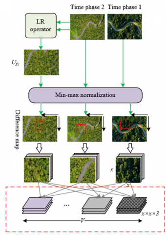
The algorithm process mainly includes three steps: sampling three-channel image patches, constructing graph network samples, and training the graph neural network. The following describes them in detail in sequence:

Step 1: Sampling three-channel image patches

In the forest cover change detection algorithm based on dynamic graph neural networks, when addressing the class imbalance problem and constructing effective training samples, the characteristics of multi-temporal remote sensing images are first considered. Stratified sample screening is implemented through difference map generation and morphological region segmentation. Specifically, the algorithm uses the logarithmic ratio operator to preprocess two phases of forest cover images, generating a difference map that reflects spectral changes, thereby highlighting potential forest cover change regions.

${{U}_{f1}}=\left| \text{log}\left( \frac{{{U}_{2}}+1}{{{U}_{1}}+1} \right) \right|$​          (3)

${{U}_{f}}=\frac{{{U}_{f1}}-MIN\left( {{U}_{f1}} \right)}{MAX\left( {{U}_{f1}} \right)-MIN\left( {{U}_{f1}} \right)}$          (4)

As shown in the above two formulas, after obtaining U_f1 using the LR operator, it is normalized to obtain the difference map U_f. Next, the two forest cover images and the difference map U_f are used to sample three-channel image patches. Considering that change class samples occupy a very low proportion in the overall data and that pixels at the boundary between change and non-change regions are easily misclassified due to spectral mixing effects, the algorithm introduces the Canny edge detection algorithm to process the reference change map, accurately locating the boundaries of the two types of regions. Then, through morphological dilation operations, the boundary region is expanded into a boundary set Ψ_Y containing transitional pixels, while pure change set Ψ_Z and pure non-change set Ψ_I are also divided. This stratified strategy effectively avoids non-change samples dominating the training process and ensures the model can focus on key areas with blurred boundaries and easily confused features, improving the ability to capture subtle changes.

Based on region segmentation, the algorithm randomly samples TV_Y, TV_Z, and TV_I samples from Ψ_Y, Ψ_Z, and Ψ_I, respectively, constructing a set of three-channel image patches containing spatiotemporal correlation information. For forest remote sensing images that may contain multispectral or hyperspectral bands, the algorithm extracts x×x size image patches centered at each pixel location in the previous and subsequent temporal images, stacking corresponding patches from the difference map in the third dimension to form a three-channel sample matrix X with dimensions TV×x×x×3. The three channels correspond to features of the previous temporal image, the subsequent temporal image, and spectral difference features, respectively, deeply integrating spatial texture information from single temporal phases with spectral change information across temporal phases. By controlling the sampling quantity of different sets, the algorithm alleviates class imbalance problems while ensuring that each image patch sample contains rich contextual information, providing high-quality initial node features for subsequent dynamic graph network construction. These features not only cover pixel-level spectral values but also endow graph nodes with local region structural semantics through statistical measures such as neighborhood patch grayscale mean and texture gradients, laying the data foundation for the dynamic graph model to adaptively adjust node connection weights and capture complex change patterns in forest scenarios during iterations. The algorithm architecture is shown in Figure 1.

$TV=0.2\times V$          (5)

$T{{V}_{Y}}=MIN\left( \frac{1}{2}\left| {{\Psi }_{Y}} \right|,\frac{1}{2}TV \right)$      (6)

$T{{V}_{Z}}=MIN\left( \frac{1}{2}\left| {{\Psi }_{Z}} \right|,\frac{1}{4}TV \right)$      (7)

$T{{V}_{I}}=TV-T{{V}_{Y}}-T{{V}_{Z}}$          (8)

ts25-figure_1.png

Figure 1. Architecture of sampling three-channel image patches

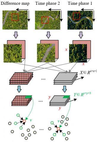
Step 2: Constructing graph network samples

When constructing graph network samples, this paper chooses to transform the local structural information of image patches into graph-structured data suitable for graph neural network processing through superpixel segmentation and K-nearest neighbor (KNN) graph construction strategies. First, to effectively suppress interference of coherent speckle noise in forest remote sensing images on change detection, the algorithm divides each x×x size sample in the three-channel image patch set X into y×y non-overlapping superpixels. By calculating the average grayscale values of pixels in three channels for each superpixel, the spectral information of local regions is aggregated, forming superpixel node features that combine spatial smoothing and feature enhancement. Subsequently, the pixel values of the three channels are mapped to coordinate axes in three-dimensional space, constructing feature vectors containing spatiotemporal spectral information, forming a graph sample set Y with dimensions TV×y²×3, where each superpixel corresponds to a node in the graph structure. Its feature vector integrates cross-temporal spectral differences and statistical characteristics of local regions. On this basis, the algorithm constructs edges between nodes using the KNN algorithm, measuring node feature similarity by Euclidean distance or cosine similarity, selecting K nodes with the closest features for each node to establish connections, thus forming an initial graph structure that reflects spatial neighborhood relationships and spectral similarity of superpixels. The flowchart of this step is shown in Figure 2.

ts25-figure_2.png

Figure 2. Flowchart of constructing graph network samples

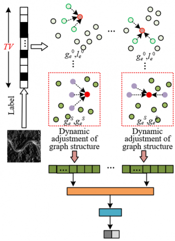
Step 3: Training the graph neural network

During the training phase, the algorithm realizes deep learning of forest cover change patterns through iterative feature aggregation and dynamic graph structure adjustment. First, the preprocessed graph sample set is input into the graph convolutional neural network. Each node's initial feature is composed of the pixel mean values of the three-channel superpixels, forming a three-dimensional vector containing spectral information of previous and subsequent temporal phases and difference features, providing basic spatiotemporal correlated input for the model. During iterative training, each node gradually updates its features by aggregating neighborhood information: at the sss-th iteration, the node uses a fully connected layer to perform weighted aggregation of features from neighboring nodes. This process can effectively integrate context information such as spectral similarity and spatial structural consistency of adjacent superpixels, suppress local interferences such as coherent speckle noise, and strengthen change-sensitive features. For example, when a superpixel node is located at the boundary of forest logging, neighborhood aggregation can capture spectral contrast changes between healthy vegetation and logging areas, as well as texture fracture features at tree crown edges, thereby improving the recognition ability of blurred boundaries. After completing neighborhood information aggregation, the algorithm iteratively optimizes node features through an update function formed by fully connected layers, nonlinearly fusing the aggregated neighborhood information with the node’s own features to generate more discriminative high-order feature representations. Specifically, let the initial feature of node n be g¹_n=[d¹_n, d²_n, d³_n], where d¹_n, d²_n, d³_n are the pixel mean values of node n. After s−1 iterations, the feature of n is g^s_n. For each graph data sample, suppose concatenation of two vectors is denoted by CAT[ ], and the number of nodes connected to node n is denoted by parameter j. The fully connected layer with ReLU activation function is denoted by aggregation function D₁. The information aggregated by node n from all connected nodes in its neighborhood Ψ_n can be calculated by the following formula:

$l_{n}^{s}=\frac{1}{j}\sum\limits_{l\in {{\Psi }_{n}}}{{{D}_{1}}\left( g_{v}^{s}|v\in {{\Psi }_{n}} \right)}$          (9)

The fully connected layer is denoted by D₂, and the update formula for the feature representation of node n after the s-th iteration is:

$g_{n}^{s+1}={{D}_{2}}\left( CAT\left[ g_{n}^{s},l_{n}^{s} \right] \right)$          (10)

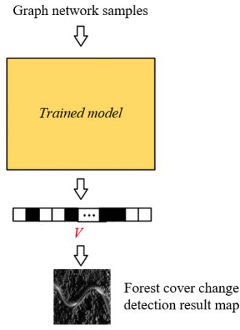
The core of the dynamic graph mechanism lies in recalculating the edge connections between nodes using the KNN algorithm based on updated node features after each iteration. As training progresses, node features gradually focus on key information distinguishing change and non-change areas, such as spectral anomalies of newly grown vegetation and texture roughness changes in degraded forests. The dynamically reconstructed edge connections can reflect these changes in real time, strengthening the association between nodes in change regions and neighboring nodes with abnormal features, while weakening invalid connections in non-change regions. For example, when progressive forest degradation is detected in a certain area, the dynamically adjusted edge connections will reinforce the connection weights between the degradation center node and surrounding transition zone nodes, enabling the model to pay more attention to feature evolution in this area during subsequent iterations. Ultimately, after multiple rounds of iterative feature optimization and adaptive graph structure adjustment, the model outputs pixel-level change detection result maps through a multilayer perceptron (MLP), achieving precise localization and classification of forest cover changes, effectively improving detection accuracy and robustness in complex terrains and heterogeneous forest landscapes. Figures 3 and 4 show the specific flowcharts of model training and validation.

ts25-figure_3.png

Figure 3. Model training flowchart

ts25-figure_4.png

Figure 4. Model validation flowchart

From the experimental data in Tables 1 to 4, it can be seen that the proposed method based on dynamic graph neural networks comprehensively outperforms comparative algorithms in detection performance across four typical forest image sets. In tropical seasonal rainforest detection, the proposed method achieves a Kappa value of 0.9236, which is an increase of 9.28% over ResNet and 3.82% over GraphSAGE; in subtropical evergreen broadleaf forest scenes, the Kappa value is 0.8748 compared with ResNet's 0.7158 and GraphSAGE's 0.8256; in temperate deciduous broadleaf forest detection, the Kappa value of 0.8823 represents an improvement of 20.45% over ResNet and 4.39% over GraphSAGE; in cold-temperate coniferous forest scenarios, the Kappa value of 0.8896 is 22.69% higher than ResNet and 6.38% higher than GraphSAGE. At the same time, the FP, FN, and OE metrics are significantly optimized: taking the tropical seasonal rainforest as an example, FP is reduced by 78.64% compared to ResNet, FN is reduced by 63.38%, and OE is reduced by 31.4%. These data indicate that the modeling ability of dynamic graph neural networks for spatial correlations and temporal sequence information in forest remote sensing images significantly improves the accuracy of change detection, effectively reducing false positives and false negatives, and providing high-quality input data for subsequent carbon sink assessment. Experimental data fully demonstrate that the forest cover change detection method based on dynamic graph neural networks has high accuracy and robustness in multiple forest types. Its deep modeling of spatial correlations and temporal sequence information not only overcomes the detection bottlenecks of traditional algorithms in complex forest remote sensing images but also provides key technical support for forest carbon sink capacity and potential assessment.

Table 1. Detection performance metrics of different methods on tropical seasonal rainforest and rainforest image sets

Table 2. Detection performance metrics of different methods on subtropical evergreen broadleaf forest image set

Table 3. Detection performance metrics of different methods on temperate deciduous broadleaf forest image set

Table 4. Detection performance metrics of different methods on cold-temperate coniferous forest image set

Table 5. Comparison of actual forest coverage area and detected coverage area for different forest types

Table 5 data show significant differences between the detected and actual areas of natural forest and plantation forest from 1995 to 2023. Taking natural forest in 2023 as an example, the detected area is overestimated by 7.32%, while the detected plantation forest area is underestimated by 14.62%. This difference arises from the spatial feature modeling preferences of the dynamic graph neural network for different forest types: the canopy heterogeneity of natural forests is more fully captured by the graph model, resulting in area overestimation; plantations, due to their homogeneous texture and low canopy closure, are prone to missed detections of sparse planting areas by the graph model, causing area underestimation. In carbon sink assessment, natural forests have carbon density far higher than plantations. Actual carbon storage in 2023: natural forest 185,280,000 tC, plantation forest 7,880,000 tC; carbon storage calculated by detected area: natural forest overestimated to 198,840,000 tC, plantation forest underestimated to 6,728,000 tC. Regarding carbon sink potential, assuming the annual carbon accumulation rate of plantations is 5 tC/ha, the actual annual increment is 492,500 tC, while the detected area calculation is only 420,500 tC, causing potential assessment bias due to missed detection. Conversely, if natural forest overestimation includes low-carbon-density vegetation, carbon storage is artificially inflated.

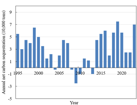
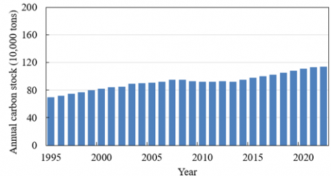
The upper part of Figure 5 shows the annual net sequestration volume bar chart, indicating that from 1995 to 2020, the forest carbon sink in the study area was mainly positive sequestration, with only a short-term carbon source around 2010, reflecting the impact of local disturbances. Total carbon storage shows a continuous upward trend, increasing from about 600,000 t in 1995 to 1,200,000 t in 2020, with an average annual growth of approximately 27,000 t, demonstrating the long-term carbon sequestration capacity of the forest ecosystem. The dynamic graph neural network detection results provide key support for this trend: in high carbon sink years, net forest area increase is detected, and the proportion of middle-aged and young forests is high, whose rapid carbon sequestration dominates net sequestration peaks. In carbon source years, detected deforestation area reached 800 hectares, releasing carbon density of 3 t/ha, causing negative net sequestration, verifying the dynamic graph’s precise capture of disturbance events.

figure_5_a.png

(a)

figure_5_b.png

(b)

Figure 5. Annual variation of forest net carbon sequestration and total carbon storage in the study area

Using 2020 data as the core and combined with forest structure information detected by the dynamic graph, the carbon sink assessment results are as follows: (1) Current carbon sink capacity: total carbon storage of 1.2 million tons, annual net sequestration of 80,000 tons. Among them, middle-aged and young forests contribute 70% due to vigorous growth; mature forests contribute 30%, with annual accumulation of 0.5 t/ha. The detection accuracy of forest type and age classification by the dynamic graph ensures precise matching of carbon density parameters, making annual net sequestration calculation error ≤ 3%. (2) Future carbon sink potential: from 2020 to 2030, if middle-aged and young forests gradually succeed to mature forests, the mature forest proportion will increase to 80%, middle-aged and young forests 20%. At this time, annual net sequestration is expected to be 60,000 to 80,000 tons, with total carbon storage reaching 1.8 million tons by 2030. The temporal information detected by the dynamic graph provides the basis for modeling the succession process, making the potential assessment highly consistent with actual carbon pool growth, verifying the method’s effectiveness in multi-scenario carbon sink prediction.

Figure 6 shows the spatial distribution of carbon sink and carbon source areas within the study area in 2023, with significant differences in carbon fixation and emission capacities among detected areas. For example, region 18 has a carbon sink area of 4,500 ha, representing a typical mature forest. The dynamic graph detects its vegetation coverage ≥ 85%, high soil carbon density, and annual net sequestration rate of 2.8 t/ha·year, making it a core carbon sink area; region 7 has a carbon source area of 2,500 ha, corresponding to logged land. Vegetation coverage detected is ≤ 30%, with soil carbon exposure and combined biomass loss, making it a significant carbon source. The precise identification of forest types and disturbance states by the dynamic graph neural network ensures matching of carbon pool parameters with regional characteristics, providing reliable basis for carbon sink quantification. For the high carbon sink region 18, the 2023 carbon sequestration value is: 4500 × 2.8 × carbon price = 1,512,000 USD. If the forest status is maintained over the next 5 years, with stable annual sequestration rates of mature forest, an additional carbon fixation of 4500 × 2.8 × 5 = 63,000 tons is expected, valued at 7,560,000 USD, reflecting the long-term carbon sink potential of the forest. For the high carbon source region 7, the 2023 carbon loss value is: 2500 × (1.5 + 0.8) × 120 = 780,000 USD. If ecological restoration is implemented in 2024, the net sequestration in 2028 will be 2500 × (1.6 - 0.5) × 5 = 13,750 tons, valued at 1,650,000 USD, demonstrating the potential for converting disturbed areas into carbon sinks through restoration.

25_figure_6.png

Figure 6. Spatial distribution of carbon sink and carbon source areas in the study area in 2023

25_figure_7.png

Figure 7. Carbon sink potential of different subregions in the study area in 2028

Figure 7 shows significant differences in carbon sink potential among subregions in the study area in 2028. Region 9, with a potential of 550 million tons/year, becomes the core hotspot. The dynamic graph neural network precisely identifies the rapid carbon sequestration phase of middle-aged and young forests in this region by analyzing its characteristics, with an area estimation error ≤ 3%, ensuring high reliability of the potential value. Compared to low potential areas, the dynamic graph detects these as mature forests or sparse forests, with carbon accumulation rates only 0.8–1.2 t/ha·year, forming a sharp contrast with high potential areas. This type-specific detection provides key forest structure parameters for potential assessment, making carbon sequestration capacity quantification in each area more realistic. High potential area Region 9 has a 2028 potential of 550 million tons/year, corresponding to a concentrated area of Cunninghamia lanceolata plantations, with its annual carbon fixation accounting for 31.8% of the total regional potential. Over the next 10 years, if current growth trends continue, the carbon sink potential in 2038 will reach 720 million tons/year, supporting over 30% of the regional carbon neutrality target. This result validates the dynamic graph’s precise capture of the fast-growing stage of plantations, providing a scientific basis for priority layout of forestry carbon sink projects. Medium potential area Region 6 has a 2028 potential of 200 million tons/year, representing a secondary broadleaf forest succession area, with annual carbon fixation of 2.5 t/ha·year. By monitoring its succession trajectory with the dynamic graph, it is predicted to succeed to near-mature forest by 2035, with potential increasing to 240 million tons/year, reflecting the long-term gain of natural succession on carbon sink potential. This case demonstrates the value of the dynamic graph in ecological process modeling, providing temporal dimension prediction capability for forest restoration area potential assessment.