Abdulhadi Altherwi*![]() | Emad Ghandourah
| Emad Ghandourah![]() | Md. Mottahir Alam
| Md. Mottahir Alam![]() | Shams Tabrez Siddiqui
| Shams Tabrez Siddiqui![]()
© 2025 The authors. This article is published by IIETA and is licensed under the CC BY 4.0 license (http://creativecommons.org/licenses/by/4.0/).
OPEN ACCESS
The incorporation of renewable energy sources into contemporary power systems necessitates accurate management of the demand-supply equilibrium, highlighting the critical role of smart grids. Signal processing techniques play a crucial role in improving load forecasting by refining feature extraction, noise reduction, and classification. This study introduces an innovative signal processing-driven approach for intelligent load forecasting in smart grids, utilizing Artificial Neural Networks (ANN) optimized by the Smart Flower Water Wave Optimization (SFWWO) algorithm. The SFWWO combines Water Wave Optimization (WWO) and Smart Flower Optimization Algorithm (SFOA) to enhance forecasting accuracy and reliability. Additionally, key signal processing techniques, such as feature selection using Motyka and Ruzicka metrics and fusion via Dice Similarity, ensure improved data preprocessing and classification. The ANN_SFWWO model outperforms existing methods, achieving the lowest RMSE (0.225), MSE (0.040), and MAPE (0.770) on the ERCOT Load Data. These findings highlight substantial improvements in energy efficiency, noise-resistant forecasting, and grid stability, underscoring the role of advanced signal processing techniques in optimizing smart grid operations.
feature selection, fusion techniques, time-series data preprocessing, load forecasting, signal processing, smart grids, neural networks, heuristic optimization
Accurate load forecasting plays a crucial role in ensuring the stability, efficiency, and resilience of smart grid systems. As modern power networks transition toward renewable energy integration and decentralized power generation, the complexity of forecasting future demand increases. Traditional forecasting methods, such as statistical and time-series models, often fail to capture the nonlinear and dynamic nature of energy consumption in smart grids, leading to suboptimal performance. Consequently, researchers have turned to computational intelligence techniques, such as Artificial Neural Networks (ANNs), which have demonstrated superior ability in recognizing complex patterns and relationships in energy demand data [1].
In recent years, signal processing techniques have emerged as a key enabler for improving the accuracy and robustness of load forecasting models [2]. These techniques include filtering, noise reduction, feature extraction, and classification, all of which enhance the quality of data used for predictive modelling [3]. In particular, wavelet transforms have been widely used to decompose complex time-series data, enabling better analysis and trend identification in power demand patterns [4]. However, the fluctuating contribution of renewable energy sources—such as solar and wind power—introduces additional forecasting challenges, necessitating adaptive and intelligent optimization techniques [5].
Despite the advantages of ANN-based forecasting, several limitations persist. First, traditional ANN models struggle with hyperparameter tuning, overfitting, and slow convergence when applied to large-scale smart grid datasets [6]. Second, selecting the most relevant features from high-dimensional load datasets remains a challenge, as irrelevant or redundant features can degrade forecasting performance [7]. Finally, many existing forecasting models lack adaptability to rapidly changing grid conditions, reducing their effectiveness in real-world applications [8].
To address these challenges, this study introduces an advanced load forecasting model that integrates signal processing techniques with heuristic optimization. Specifically, we propose an ANN-based forecasting framework optimized using the Smart Flower Water Wave Optimization (SFWWO) algorithm, a novel hybrid approach that combines Sun Flower Optimization Algorithm (SFOA) and Water Wave Optimization (WWO). SFOA mimics the adaptive growth patterns of plants to improve search efficiency and convergence speed [9] while WWO simulates the propagation and refraction of water waves to find optimal solutions in large search spaces [10].
By integrating these two nature-inspired optimization techniques, SFWWO enhances the learning capability of ANN models, ensuring improved forecasting accuracy and computational efficiency [11]. Signal processing plays a critical role in enhancing the quality of input data for ANN training. In this study, we employ:
• Feature Extraction: Utilizing Ruzicka and Motyka similarity metrics to select key influencing factors, such as weather conditions, time variations, and user consumption patterns [12].
• Feature Fusion: Applying the Dice similarity coefficient to combine extracted features, reducing redundancy and enhancing classification accuracy [13].
• Noise Filtering: Using advanced filtering techniques to remove anomalies in historical load data, improving the robustness of forecasting models [14].
By combining signal processing methods with deep learning and optimization, our approach effectively handles noisy, high-dimensional, and non-stationary energy datasets, ensuring reliable load predictions in dynamic smart grid environments.
The main contributions of this study can be summarized as follows:
• Development of an Enhanced ANN-Based Forecasting Model: ANN is optimized using SFWWO, significantly improving prediction accuracy and computational efficiency.
• Integration of Signal Processing Techniques for Data Preprocessing: Advanced feature selection, fusion, and filtering enhance the quality and relevance of input features for ANN training.
• Comprehensive Evaluation on Real-World Smart Grid Datasets: The proposed model is validated using datasets from ISO New England and ERCOT, demonstrating its robustness across diverse grid conditions.
• Advancement in Smart Grid Energy Management: The model supports scalable, noise-resistant, and adaptive forecasting, contributing to efficient energy distribution, reduced power waste, and enhanced grid stability.
The flow of the paper is arranged as follows: Section 2 provides a comprehensive review of existing load forecasting methodologies and the role of signal processing in smart grid applications. Section 3 introduces the system model, detailing the dataset and preprocessing techniques. Section 4 describes the proposed ANN_SFWWO framework, focusing on training, feature selection, and optimization. Section 5 presents experimental results, including comparative analysis with existing methods. Finally, Section 6 summarizes the research with main outcomes and prospective directions for impending research.
Zhang et al. [6] introduced an innovative real-time prediction model for smart grids, integrating a convolutional neural network (CNN) attention mechanism with bi-directional long- and short-term memory (BiLSTM). This model excels in spatiotemporal feature extraction, yielding higher prediction accuracy and enhanced adaptability compared to conventional methods such as ARMA and decision trees. To refine feature selection, Bayesian optimization is incorporated, allowing the model to efficiently learn from real-time load data. By utilizing real-time power system data—including power consumption, load variations, and meteorological factors—the model ensures accurate future load predictions. Additionally, Bayesian optimization fine-tunes hyperparameters, further strengthening predictive accuracy. Despite its efficiency in estimating real-time power loads for operational and dispatch applications, the model's computational complexity may affect execution speed.
Rabie et al. [7] proposed an Optimal Load Forecasting Strategy (OLFS), which leverages artificial intelligence (AI) for smart grid demand prediction. This methodology involves an initial preprocessing phase where feature selection and outlier detection are performed before forecasting. Advanced Leopard Seal Optimization (ALSO), a bio-inspired optimization technique, is employed for feature selection, while Interquartile Range (IQR) is utilized for detecting and eliminating statistical anomalies. For forecasting, the approach integrates the Weighted K-Nearest Neighbor (WKNN) algorithm, optimizing predictive performance while reducing root mean square error (RMSE). However, deep learning (DL) techniques were not explored, potentially limiting further improvements in forecasting accuracy.
To address the challenges in short-term power load forecasting, Wen et al. [8] designed a computational framework that integrates multiple deep learning (DL) models. This hybrid approach employs Gated Recurrent Unit (GRU) networks, which effectively capture long-term dependencies in time-series energy data. By leveraging pattern recognition and feature extraction, the model minimizes forecast errors and enhances accuracy, proving beneficial for grid planning and energy management. Furthermore, an attention mechanism is incorporated to prioritize key input components that significantly influence load prediction outcomes, improving model performance.
A hybrid short-term electric load forecasting model was introduced by Hafeez et al. [9], incorporating an improved Modified Mutual Information (MMI) technique. This method refines data preprocessing and feature selection by extracting abstract features from historical load records. The model is built upon a Factored Conditional Restricted Boltzmann Machine (FCRBM), a deep learning-based forecasting module. Additionally, Genetic Wind-Driven Optimization (GWDO) is employed to fine-tune model parameters, enhancing forecasting accuracy and convergence rates. Despite its effectiveness, the model’s high computational scalability presents a challenge in large-scale implementations.
To further enhance forecasting precision and system performance, Aly [10] developed a hybrid forecasting method by integrating multiple machine learning techniques with clustering algorithms. The model incorporates six forecasting schemes, each utilizing unique combinations of Kalman Filtering (KF), Wavelet Transformation, ANN, and Wavelet Neural Networks (WNN). While the approach achieves high accuracy levels, its training process is computationally intensive, requiring significant resources.
Mansoor Ali et al. [11] proposed a hybrid forecasting framework named WLANFIS, which merges Adaptive Neuro-Fuzzy Inference System (ANFIS), Neural Networks (NN), and Weighted Least Squares (WLS). The methodology integrates fuzzy logic and neural networks, where an optimized dataset—derived from NN and WLS—determines the optimal membership functions and fuzzy set boundaries. This approach effectively mitigates overfitting issues, yet its inability to integrate Deep Neural Networks (DNN) with Kalman filter-based state estimation remains a limitation.
In the domain of load and price forecasting, Naz et al. [12] developed two predictive models: Enhanced Logistic Regression (ELR) and Enhanced Recurrent Extreme Learning Machine (ERELM). ELR represents an optimized variant of logistic regression, whereas ERELM employs the Grey Wolf Optimizer (GWO) for fine-tuning model weights and biases. The study also utilized Recursive Feature Elimination (RFE), Relief-F, and Classification and Regression Trees (CART) for feature selection and extraction. While the models achieved superior forecasting accuracy with larger datasets, their high computational complexity posed a challenge for real-time applications.
Dai and Zhao [13] developed a hybrid model incorporating intelligent techniques to optimize parameters and select features for power load forecasting. Given the increasing impact of real-time pricing on electricity consumption patterns, they considered real-time pricing and other influential variables as candidate features. Minimal redundancy maximal relevance was applied to extract informative features, while the weighted gray relation projection approach was used to select historical load sequences, making the selection more general. Finally, repulsion particle swarm optimization (PSO) and second-order oscillation were employed to optimize support vector machine parameters. Although, the approach requires more training iterations, it achieves noticeably higher accuracy.
The key challenges faced by existing methods:
Data quality and availability issues, complexity of Smart Grids, and non-linear relationships between load demand and variables, like weather and time hinder accurate forecasting. Uncertainty and variability of load demand, scalability, and interpretability of models also pose challenges. Real-time processing requirements, integration with other systems, and cybersecurity concerns add to the complexity. Compliance with regulatory and policy frameworks, balancing accuracy and computational efficiency, and handling special events like weather anomalies or grid failures are also crucial. Moreover, long-term forecasting needs and accounting for distributed energy resources and electric vehicle charging must be addressed. To overcome these challenges, advanced forecasting techniques, data preprocessing, and robust modeling approaches are necessary. By addressing these challenges, Intelligent Load Forecasting can support efficient and reliable grid operations, optimize energy distribution, and enable a sustainable energy future. Effective solutions will require collaboration among researchers, industry experts, and policymakers to develop and implement innovative forecasting methods and technologies.
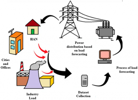
Figure 1 illustrates the proposed signal processing-enhanced load forecasting framework for smart grids. The model employs smart energy meters to collect real-time power consumption data, followed by advanced preprocessing techniques such as missing value imputation and noise filtering. Extracted features undergo selection and fusion using Ruzicka and Motyka similarity metrics, which refine classification accuracy.
The unpredictable nature of renewable energy sources, along with consumer-driven demand fluctuations, necessitates an adaptive forecasting model. The proposed ANN_SFWWO framework effectively mitigates these uncertainties by learning complex patterns and adjusting predictions accordingly, ensuring optimal grid stability and energy efficiency.
Figure 1. Load forecasting in smart grids
This study introduces a innovative approach for load forecasting in smart grids by integrating an Artificial Neural Network (ANN) with the SFWWO algorithm. The SFWWO algorithm synergistically combines the strengths of Smart Flower Optimization Algorithm (SFOA) and WWO, enabling efficient search for optimal solutions and robust handling of complex data patterns.
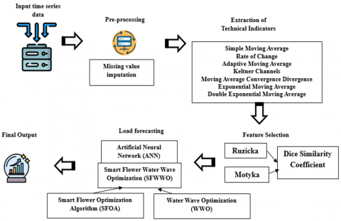
Figure 2. Preview of load forecasting in smart grids using ANN_SFWWO
The methodology follows a structured approach starting with data collection from smart grids. This is followed by missing value imputation and preprocessing to enhance data integrity. Feature extraction techniques identify key technical indicators such as Simple Moving Average (SMA), Rate of Change (ROC), and Adaptive Moving Average (AMA). Next, feature selection is performed using Ruzicka analysis to determine relevance, while Motyka analysis assesses feature importance. The Dice similarity coefficient is then applied for feature fusion, ensuring redundancy reduction and improved classification accuracy. The final forecasting is executed using ANN, which is optimized by SFWWO to improve model training, accelerate convergence, and enhance predictive performance. Figure 2 illustrates the overall workflow of the ANN_SFWWO-based load forecasting approach which can be summarized as follows:
Preprocessing and Feature Extraction: The preprocessing stage enhances reliability by handling missing values, filtering noise, and detrending data. Imputation ensures completeness, reducing bias and improving accuracy. Key technical indicators like SMA, ROC, and MACD capture load variations and trends in smart grid data [14].
Feature Selection and Fusion: To enhance forecasting accuracy, extracted features are selected and fused using Ruzicka for relevance, Motyka for significance, and Dice similarity to refine fusion, remove redundancy, and improve classification.
ANN Training with SFWWO Optimization: The ANN model, optimized with SFWWO, merges SFOA’s adaptability and WWO’s search efficiency for precise weight tuning, ensuring faster convergence and higher accuracy in load forecasting. Designed for dynamic grid conditions, ANN_SFWWO offers a reliable solution for smart grid energy management.
4.1 Acquisition of time series data
The time series data is regarded as an input for additional processing in this context. The dataset, including multiple series data is provided by,
$A=\left\{ A{{}_{h1}},{{A}_{h2}},...,{{A}_{hp}},...,{{A}_{hv}} \right\}$ (1)
where, Ahv is the vth time series data, Ah1 is the initial time series data at time period h, and Ahp is the pth time series data for further processing.
4.2 Pre-processing
Pre-processing of time series data is crucial for load forecasting in smart grids as it ensures accurate and reliable predictions by handling missing values, removing noise and outliers, normalizing and scaling data, detrending and adjusting for seasonality, extracting relevant features, and improving model performance. This enables smart grids to optimize energy distribution, manage peak demand, and integrate renewable energy sources effectively. By pre-processing time series data, smart grids can improve forecast accuracy, reduce energy waste, and enhance overall grid efficiency, ultimately leading to cost savings, improved customer satisfaction, and a more sustainable energy future.
In order to reduce the amount of redundant data, the time series data Ahp is pre-processed using missing value imputation. In addition, it reduces bias and prediction errors by substituting estimated values for missing data points to produce a complete dataset. Additionally, during the pre-processing stage, the raw data input is converted into a readable data format, greatly improving the prediction accuracy. In this case, feature average in non-missing data is used to identify missing values. At last, the absent values are filled in. Here, the term Q represents the pre-processed data output.
4.3 Extraction of technical indicators
Extraction of technical indicators is important for load forecasting in smart grids because it transforms raw time series data into meaningful features that capture patterns, trends, and seasonality, enabling accurate predictions. Technical indicators, such as Simple Moving Average (SMA), Rate of Change (RoC), Adaptive Moving Average, Keltner Channels, Moving Average Convergence Divergence (MACD), Exponential Moving Average (EMA), and Double Exponential Moving Average (DEMA), which are extracted from Ahp for forecasting. By extracting these indicators, smart grids can identify key factors influencing load demand, improve forecast accuracy, and optimize energy management, ultimately leading to efficient grid operations, reduced energy waste, and enhanced customer satisfaction. Table 1 lists the technical indicators parameter setting.
Table 1. Configuration of technical indicators
|
Technical Indicators |
Parameters |
|
SMA |
Window size = 10 time-steps |
|
EMA |
Smoothing constant S=0.2, Window size = 10 |
|
DEMA |
Window size = 10 time-steps |
|
RoC |
Look-back period = 5-time steps |
|
AMA |
Fast EMA window = 2, Slow EMA window = 30 |
|
MACD |
Fast EMA = 12, Slow EMA = 26, Signal line EMA = 9 |
|
ATR |
Window size=10 |
|
Keltner Channels |
EMA window = 20, ATR window = 10, Multiplier = 2 |
SMA: The SMA [14] is calculated by summing up the load values over a specified period, and then dividing by the total count of time periods and the SMA indicator output is denoted as ${{b}_{1}}$.
EMA: EMA [14] is expressed as the weighted average of recent load values, giving more weight to recent observations, to better forecast load in smart grids.
$EMA=\left( a-EM{{A}_{a}} \right)*S+EM{{A}_{a}}$ (2)
The weighted average for the current period is denoted by a, the EMA for the previous period is shown by EMAa, the smoothing constant is denoted by S, and the EMA indicator output is indicated by b2.
DEMA: DEMA [14] is an indication that offers a smoothed mean with less lag than EMA. It is symbolized as,
$DEMA=\left( 2*EMA(t) \right)-\left( EMA(t)\,of\,EMA(t) \right)$ (3)
The DEMA indicator notation is b3.
ROC: ROC [14] calculates the percentage change in load values over a specified period. The result is a measure of the rate of change in load, which can be used to identify trends, patterns, and anomalies in load data.
$ROC=\left( \left( {d}/{e}\; \right)-1.0 \right)*100$ (4)
where, d is the current load value, and $e$signifies the previous load value from a specified time ago, and the ROC indicator output is expressed as b4.
MACD: The differences between the two MAs of different periods, such as fast MA and slow MA, are taken into account while computing the MACD indicator [15]. The MACD indicator can be written as:
${{b}_{5}}=FastMA-SlowMA$ (5)
where, FastMA stands for the shorter MA, SlowMA for the longer MA, and the MACD indicator is shown as b5.
AMA: Another technical indicator that uses scalable constants rather than set constants to smooth data is the AMA. The symbol for this indicator is b6.
Keltner Channels: The Keltner channel is a volatility-based technical indicator that typically displays three lines: an upper band, a middle line, and a lower band. The EMA is the middle line of the Keltner channel, with the other two bands situated above and below it. Keltner channel equations are therefore represented by,
$W={{E}_{1}}$ (6)
${{B}_{R}}={{E}_{1}}+2*D$ (7)
${{B}_{J}}={{E}_{1}}+2*D$ (8)
where, D stands for average true range, W for the center line of the keltner channel, BR for the upper band, BJ for the lower band, and E1 for the EMA. The indication of the Keltner channel is denoted by b7.
Rate of Change: The ROC is used to estimate the rate of alternation or change in load quality for a previous time interval.
${{b}_{8}}=\frac{X\left( q \right)}{X\left( q-m \right)}*100$ (9)
where, load quality is represented by X, load quality at a given period q by X(q), and load quality variation over time by X(q-m). The ROC curve, represented by b8.
Thus, joining the whole extracted technical indication yields the final feature vector of the technical indicator. Consequently, the expression is modeled as,
$G=\left\{ {{b}_{1}},...,{{b}_{8}} \right\}$ (10)
As a result, the next step in the feature selection procedure uses the input as the retrieved technical indicator G.
4.4 Feature selection
Feature selection is crucial after extracting technical indicators for load forecasting in smart grids as it reduces dimensionality, removes irrelevant features, improves model interpretability, enhances model performance, and reduces the risk of multicollinearity. By selecting the most relevant features, understand the relationships between technical indicators and load demand, improve model accuracy, reduce noise, and increase training speed. This step helps build a more robust, accurate, and interpretable load forecasting model, enabling smart grids to optimize energy management, reduce energy waste, and enhance customer satisfaction. Here, the retrieved technical indicator output $G$ is considered as input. In this case, the dice similarity metric is fused with the Ruzicka and Motyka to choose the essential features.
Ruzicka similarity: The Ruzicka similarity (also known as weighted Jaccard similarity) measures the degree of overlap between feature distributions while accounting for their magnitude differences. It has the potential to analyze uneven data distribution, which makes it suitable for smart grid applications where the load and energy patterns vary continuously. This is then expressed as:
${{P}^{RUZ}}=\frac{\sum\limits_{g=1}^{c}{\min ({{N}_{g}}{{K}_{g}})}}{\sum\limits_{g=1}^{c}{\max ({{N}_{g}}{{K}_{g}})}}$ (11)
where, Ng stands for candidate features and Kg for class label. It determines the highest-value features by calculating each feature's Ruzicka similarity. Thus, Cn×q where p>q is the output.
Motyka similarity: The Motyka similarity evaluates the similarity between two data sequences. It defines ratio of summation of minimum values of corresponding components in the two data sequences to the sum of all elements, as formulated in Eq. (12). In the presented work, it was deployed for selecting relevant attributes for ANN by estimating features that are similar across various data sequences. Here, $G$ is regarded as input in this instance as well. Each pair of two input collections has its similarity calculated using the Motyka similarity, which is provided by:
${{P}^{MOT}}=\frac{\sum\limits_{g=1}^{c}{\min ({{N}_{g}}{{K}_{g}})}}{\sum\limits_{g=1}^{c}{\left( {{N}_{g}}+{{K}_{g}} \right)}}$ (12)
where, Kg denotes the target class and Ng denotes candidate features. It chooses the best features with the highest value after calculating each feature's Motyka similarity. Fn×r where p>r is the output's symbol.
Fusion by dice coefficient: Features obtained by means of the Motyka and Ruzicka poses several types of representation. Thus, efficiency can be completely destroyed by a simple concatenation. Therefore, the majority of rich detail information is encoded in the characteristics that the Ruzicka obtains, while the Motyka gathers context information. In order to create features that are more effective, the output:
${{P}^{DICE}}=\frac{2\sum\limits_{g=1}^{c}{{{N}_{g}}{{K}_{g}}}}{\sum\limits_{g=1}^{c}{N_{g}^{2}}+\sum\limits_{g=1}^{c}{K_{g}^{2}}}$ (13)
where, Kg stands for Target class and Kg stands for candidate features, which are the output features produced by combining Ruzicka and Motyka. Cn×k represents the output in the case where (q+r)>l.
4.5 Load forecasting using ANN_SFWWO
Load forecasting plays a vital role in enhancing energy management and minimizing energy waste within smart grids. By predicting energy demand with high precision, smart grids can dynamically adjust supply to meet demand in real-time, ensuring efficient and reliable power distribution while optimizing overall grid performance. In the proposed work, an optimized framework was developed for accurately predicting loads. The designed framework leverages the optimization capacity of hybrid optimizer named “Sun Flower Water Wave Optimization (SFWWO)” with ANN. The proposed SFWWO combines the efficiency and advantages of SFOA and WWO. SFOA is a meta-heuristic optimization technique inspired from the characteristics of sunflowers for searching the best orientation towards the sun. In this algorithm, the pollination process is simulated based on random generation of seeds, which ensures adaptability to real-world constraints. Also, this algorithm outperformed the conventional optimization techniques such PSO, genetic algorithm (GA), etc., by easily solving the complex problems in different fields. On the other hand, WWO is a nature-inspired meta-heuristic algorithm modeled based on the shallow water wave theory for resolving the world optimization problems. This approach includes water wave phenomena like refraction, propagation and refraction. This approach has the efficiency of searching in a high-dimensional solution space, which makes it an optimal solution for problems in large networks like smart grids. Also, this approach regulates the searching process with minimal control parameters, reducing the computational power and computational time. These advantages make the WWO approach more efficient than conventional techniques like PSO, GA, ACO, etc. [15, 16]. Thus, the integration of SFOA and WWO into single optimization algorithm ensures adaptability, complex problem solving, less computational demands and high-dimensional searching, making it a suitable solution for smart grid-based problems. This synergy enables smart grids to better anticipate and respond to changing energy demands, reducing the risk of power outages and minimizing energy waste. By improving load forecasting, smart grids can optimize energy management, reduce costs, and enhance customer satisfaction, making this research essential for the development of high-performance renewable energy models.
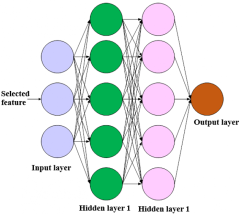
Structure of ANN: An Artificial Neural Network (ANN) [17] is an adaptable model capable of identifying patterns by repeatedly analyzing data, allowing it to generalize and make predictions on previously unseen information. In this context, Cn×k serves as the input for the ANN. In supervised learning, the network is guided by human intervention, where specific data relationships are defined to enable accurate learning and decision-making. The network attempts to learn the input-output connection by adjusting its free parameters after being provided a set of inputs and corresponding desired outputs. Here, the activation function u(z) is the sigmoid function, which can be found by:
$u\left( z \right)=\frac{1}{1+\exp \left( -z \right)}$ (14)
$z=\sum\limits_{f=1}^{j}{{{x}_{if}}{{l}_{f}}}+{{\alpha }_{i}};i=1\,to\,p$ (15)
$z=\sum\limits_{i=1}^{j}{{{x}_{ib}}{{q}_{i}}}+{{\alpha }_{b}};b=1\,to\, \text{K}$ (16)
where, α is threshold, x is synaptic weight, l is input node value, p is hidden note value, p is number of hidden nodes, f is number of output nodes, and j is the number of input nodes. Figure 3 shows the structure of ANN.
The learning algorithm of a back-propagation neural network consists of two phases.
Phase I: The network input layer is given with a constraining input pattern.
Phase II: After that, the input pattern is spread throughout the network's layers until the output layer generates the output pattern. When the produced pattern does not match the expected output, an error is calculated and then propagates backward from the output layer back to the input layer across the network. This backpropagation process adjusts the network’s weights, refining them based on error magnitude and optimization criteria, ultimately enhancing the model’s accuracy and performance. In contrast to other neural networks, a back-propagation neural network is based on the activation function, the connections between the neurons, and the adjustment of weights by the intended output level. A back-propagation network typically consists of three or more tiers in a multi-layer architecture. Every neuron in each layer is connected to every other neuron in the forward levels that surround it, and the layers are coupled.
Figure 3. ANN architecture
Training ANN by SFWWO: Although ANN offers promising results in pattern recognition, its prediction performances highly rely on the appropriate selection of hyperparameters in its training phase. Hence, hyperparameter optimization was introduced for finding the best combination of hyperparameters for a machine learning model to maximize its performance. In the presented work, the ANN training is performed using SFWWO, a novel hybrid algorithm combining SFOA [18] and WWO [19]. Sunflowers serve as the inspiration for the SFOA, which clarifies and idealizes the growth of young sunflowers. The outcomes validated the ability and effectiveness in identifying the best. It reveals its usefulness in resolving practical issues with ambiguous search spaces. It helps with a range of engineering design problems. Flowers bloom and grow towards sunlight, maximizing their exposure to light and nutrients. This process is optimized through natural selection, ensuring the fittest flowers survive and reproduce. Meanwhile, the WWO propagates and interacts with their environment, adapting to obstacles and boundaries. This algorithm captures this dynamic behavior to search for optimal solutions. Thus, the mixture of SFOA and WWO aids to elevate overall efficiency and leads to obtain global optimal solution. The steps of SFWWO are described below.
Initialization: The search agent update in SFOA is performed using an immature sunflower growth model and is expressed as,
$M=\left[ \begin{matrix}{{s}_{1,1}} & {{s}_{1,2}} & \cdots & {{s}_{1,\dim}} \\{{s}_{2,1}} & {{s}_{2,2}} & \ldots & {{s}_{2,\dim}} \\ \vdots & \vdots & \vdots & \vdots \\{{s}_{H,1}} & {{s}_{H,2}} & \ldots & {{s}_{H,\dim}} \\\end{matrix} \right]$ (17)
where, H denotes the quantity of young sunflowers and $\dim$ the quantity of variables.
Identify error: To get the optimal answer, the error in each solution is found and is provided as:
$MSE=\frac{1}{k}\,\left[ \sum\limits_{p=1}^{k}{{{\beta }_{p}}-L} \right]$ (18)
where, k is the total amount of data, βp is the estimated output, and L is the output generated by the ANN.
Immature sunflower growth simulation: According to SFOA, two modes, like sunny and cloudy or rainy, are employed to simulate the growth of immature sunflowers. The initial mode can be written as:
$I_{new,M}^{y+1}=\left\{ \begin{align}& I_{old,M}^{y}+o\times \operatorname{Sin}(\eta )\times \left[ Dzp\times I_{best,M}^{y}-I_{old,M}^{y} \right] \\& I_{old,M}^{y}+o\times \operatorname{Sin}(\eta )\times \left[ I_{best,M}^{y}-I_{old,M}^{y} \right] \\\end{align} \right.$ (19)
where, o denotes the damping parameter, $I_{old,M}^{y}$ discloses the old element in iterations, and $I_{best,M}^{y}$ is the best element in iterations. The stopping of the stem elongation of the sunflower is reflected by the damping attribute, which is expressed as:
$o=dam{{p}_{\max }}-y\times \frac{(dam{{p}_{\max }}-dam{{p}_{\min }})}{{{y}_{\max }}}$ (20)
Here, y is the current iteration, dampmax and dampmin represent the maximum and lowest values of the damping parameter, and ymax is the maximum number of iterations. Rainy or overcast days cause the young sunflowers to experience heliotropic effects at reduced rates. When a day is cloudy or wet, it means that Auxin has not advanced. The second option is used, where the sun attribute is set to 0, to replicate these scenarios. It is stated as:
$\begin{align}& I_{new,M}^{y+1}=I_{old,M}^{y}+o\times \operatorname{Sin}(\eta )\times \left[ I_{best,M}^{y}-I_{old,M}^{y} \right]; \\& at\,\,any\,\,hours\,day \\\end{align}$ (21)
$I_{new,M}^{y+1}=I_{old,M}^{y}\left[ 1-o\operatorname{Sin}(\eta ) \right]+o\times \operatorname{Sin}(\eta )\times I_{best,M}^{y}$ (22)
However, the SFOA has a slow convergence speed and a high memory consumption. To solve this, the WWO incorporates the SFOA to find the best solution. The revised equation derived from WWO is provided by:
${{A}_{c,\,s}}(a+1)={{A}_{c,\,s}}(a)+Gaussian\left( 0,\,1 \right).\,\delta .\,{{Z}_{s}}$ (23)
Assume, ${{A}_{c,s}}\left(a+1\right)=I_{new,M}^{y+1},and~{{A}_{c,s}}\left( a+1 \right)=I_{old,M}^{y}$ substitute in Eq. (23):
$I_{new,M}^{y+1}=I_{old,M}^{y}+Gaussian\left( 0,\,1 \right).\,\delta .\,{{Z}_{s}}$ (24)
$I_{old,M}^{y}=I_{new,M}^{y+1}-Gaussian\left( 0,\,1 \right).\,\delta .\,{{Z}_{s}}$ (25)
Substitute Eq. (25) in Eq. (22),
$\begin{align}& I_{new,M}^{y+1}=I_{new,M}^{y+1}-Gaussian\left( 0,\,1 \right).\,\delta .\,{{Z}_{s}}\left[ 1-o\operatorname{Sin}(\eta ) \right] \\& +o\times \operatorname{Sin}(\eta )\times I_{best,M}^{y} \\\end{align}$ (26)
$\begin{align}& I_{new,M}^{y+1}-I_{new,M}^{y+1}\left[ 1-o\operatorname{Sin}(\eta ) \right]= \\& -Gaussian\left( 0,\,1 \right).\,\delta .\,{{Z}_{s}}\left[ 1-o\operatorname{Sin}(\eta ) \right]+o\times \operatorname{Sin}(\eta )\times I_{best,M}^{y} \\\end{align}$ (27)
$\begin{align}& I_{new,M}^{y+1}\left[ 1-1+o\operatorname{Sin}(\eta ) \right]= \\& -Gaussian\left( 0,\,1 \right).\,\delta .\,{{Z}_{s}}\left[ 1-o\operatorname{Sin}(\eta ) \right]+o\times \operatorname{Sin}(\eta )\times I_{best,M}^{y} \\\end{align}$ (28)
$\begin{align}& I_{new,M}^{y+1}\left[ o\operatorname{Sin}(\eta ) \right]= \\& -Gaussian\left( 0,\,1 \right).\,\delta .\,{{Z}_{s}}\left[ 1-o\operatorname{Sin}(\eta ) \right]+o\times \operatorname{Sin}(\eta )\times I_{best,M}^{y} \\\end{align}$ (29)
ANN_SFWWO final update is provided by,
$\begin{align}& I_{new,M}^{y+1}=-Gaussian\left( 0,\,1 \right).\,\delta .\,{{Z}_{s}}\left[ 1-o\operatorname{Sin}(\eta ) \right] \\& +o\times \operatorname{Sin}(\eta )\times I_{best,M}^{y}\left[ \frac{1}{o\operatorname{Sin}(\eta )} \right] \\\end{align}$ (30)
Re-compute error: Eq. (18) is used to reevaluate the error and produce the best possible solution by adjusting the ANN optimal weights.
Termination: When an iteration reaches a higher iteration count, the process ends with termination. Algorithm 1 represents the ANN_SFWWO pseudocode.
| Algorithm 1. Pseudo code of ANN_SFWWO |
|
Input: Population of Sunflower M |
|
Output: Optimal solution $I_{best,M}^{y}$ |
|
Begin |
|
Establish the existing population and initialize it |
|
Find the best possible option |
|
For=1 to ymax |
|
Use Eq. (20) to generate the damping parameter |
|
For h=1 to H |
|
Produce η |
|
For z=1 to Dim |
|
If Sun=1 |
|
Create the parameters |
|
Utilize Eq. (21) to update the population element |
|
else |
|
Create hours each day |
|
Update the population element using Eq. (30) |
|
End if Sun |
|
Revise the angle parameters |
|
ηy+1=ηy+φ |
|
End for z |
|
End for y |
|
Recalculate the optimal solution with an error |
|
Replace ${{I}_{best}}$by ${{I}_{best,new}}$if $u({{I}_{best,new}})<u({{G}_{best}})$ |
|
End for y |
|
End |
Here, the best prediction result is achieved by adjusting the ANN weight and bias using the SFWWO.
The outcomes of ANN_SFWWO load forecasting in smart grids are presented in this section.
5.1 Experimental setup
A Windows 10 (64-bit) system equipped with an Intel Core i3 processor and 4 GB of RAM was used to configure the proposed ANN_SFWWO. The presented model is executed in Python software version 3.12.6.
5.2 Dataset description
The datasets, like the Dayton GRID dataset, and formula electric (FE) grid [20] are used for load forecasting in smart grids, and are elaborated below.
Dayton GRID Dataset (D1): The Dayton GRID dataset includes hourly electricity consumption data from Dayton, Ohio, USA. It represents a less dynamic, lower-load profile, capturing hourly load values alongside temperature, humidity, dew point, time of day, and detailed energy demand records. Each record is timestamped, allowing analysis of load behavior.
FE GRID Dataset (D2): The FE GRID dataset contains energy load profiles from a densely populated and urbanized region, reflecting significant residential, commercial, and industrial consumption. It comprises hourly load data, meteorological parameters, and demand profiles. The dataset's complexity assists detailed load forecasting analysis.
Limitations due to Dataset Time Range: While this study employs recently updated datasets from Dayton and Formula Electric (FE), collected in 2024, earlier analyses included ISO New England and ERCOT data up to 2020. Given recent substantial integration of renewable energy sources, the older data may not fully reflect current load dynamics influenced by intermittent renewable penetration. Thus, while our updated datasets improve relevancy, caution is recommended when generalizing findings from the older datasets. Future research should consider using continually updated datasets reflecting real-time grid transformations to further validate model applicability and accuracy in evolving renewable energy scenarios.
5.3 Performance metrics
The performance metrics of ANN_SFWWO are evaluated by using three assessment measures: MSE, RMSE, and MAPE.
MSE: It calculates the mean of the squared deviations between the predicted and actual load values. A lower MSE value indicates better forecasting performance, with 0 being the ideal value. Eq. (18) defines the fitness function, also known as the MSE.
RMSE: It determines the square root of the mean squared deviation between the predicted and actual load values. RMSE is similar to MSE, but it's more sensitive to large errors, making it a more suitable metric for load forecasting. The lower values indicate better forecasting performance, whereas values closer to 0 indicate perfect forecasting. The expression is stated by:
$RMSE=\sqrt{MSE}$ (31)
MAPE: It calculates the mean absolute percentage variation between the predicted and actual load values. MAPE is a useful metric because it: Expresses errors as percentages, making it easy to interpret, is sensitive to relative errors, not just absolute errors, and is used to compare forecasting performance across different datasets. The MAPE formula is given below:
$\mathrm{M} A P E=\frac{100 \%}{v} \sum_{\kappa=1}^v \frac{\left|A c t_\kappa-F o r_\kappa\right|}{A c t_\kappa}$ (32)
where, $F o r_\kappa$ is the expected value, $\kappa$ is the time, $v$ is the fitted points, and $A c t_\kappa$ is the actual value.
5.4 Training and validation performances
The developed ANN_SFWWO was trained and validated using two datasets (D1 and D2). The dataset was split into 70:30 ratio for model training and test purposes. In the initial phase of ANN training, its hyperparameters are selected randomly. After a few epochs, the designed SFWWO tunes the ANN hyperparameters to their optimal value. Table 2 tabulates the ANN hyperparameters and their fine-tuned value.
Table 2. ANN hyperparameter optimization
|
Hyperparameter |
Optimized Value |
|
Model Layers |
3 |
|
Dense Layer |
1 |
|
Nodes in Layers 1, 2, and 3 |
128, 64, 32 units |
|
Loss Function |
MSE |
|
Optimizer |
SFWWO |
|
Batch Size |
32 |
|
Epochs |
100 |
|
Learning Rate |
0.001 |
|
Activation Function |
ReLU |
|
Population Size |
30 |
|
Drop Out |
0.1 |
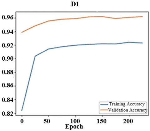
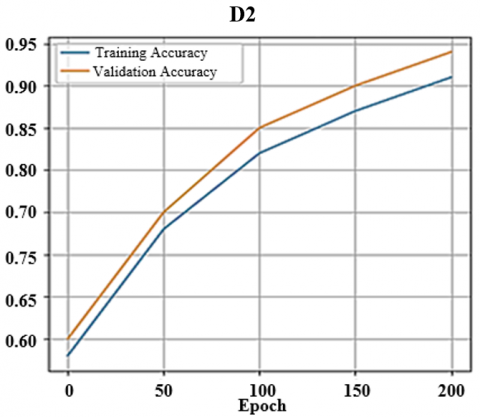
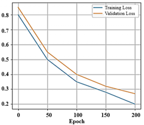
The developed model’s performances in the training and validation phases are evaluated using metrics such as accuracy and loss. Figure 4(a) and Figure 4(b) display the train and validation outcomes of the design for the D1 and D2 datasets.
Training accuracy evaluates the system’s potential of learning and understanding the patterns associated with load prediction, while validation accuracy defines how the developed model applies the learned patterns to the real-world data and make precise prediction. Train loss quantifies the difference between the predicted and actual load in smart grids on train set, while validation loss measures the error made by the system on test data. It is observed that in both cases (datasets), the proposed model obtained higher accuracy and minimum loss, highlighting its efficiency of accurately predicting loads. Also, the increase in accuracy over epochs demonstrates that the continuous fine-tuning of ANN parameters by SFWWO enhances the model’s prediction efficiency.
Figure 4. Train and test performances: (a) Accuracy, (b) Loss
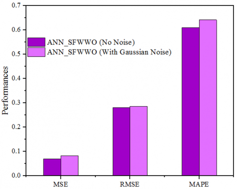
Figure 5. Performances under noisy data conditions
Furthermore, the efficiency of the developed model was assessed under noisy conditions to determine its robustness and reliability in real-world scenarios. Typically, the smart grid data contains noise attributes as it was gathered using IoT sensors and smart meters, which are prone to environmental interferences. Figure 5 presents the performance of the developed model under no-noise and noisy condition. This evaluation enables to assess how the designed ANN_SFWWO tackle real-time smart grid data. It is observed that the presented technique almost maintained stable performances under both scenarios, highlighting its applicability in real-world applications.
5.5 Comparative assessment
In this module, the performances incurred by the developed framework were compared with conventional load forecasting algorithms to validate its effectiveness and reliability in making predictions. The existing approaches used in comparative study include CNN-BiLSTM [6], WKNN-ALSO [7], FCRBM [9], ERELM [12], WLANFIS [11], Long Short Term Memory (LSTM) [21], Bidirectional Encoder Representations from Transformers (BERT) [22], and Graph Attention Network (GAT) [23]. Different datasets are used for comparative analysis with respect to assessment measures.
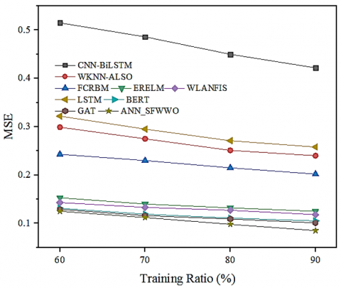
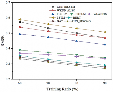
Performance comparison for D1 dataset: Figure 6 displays the comparative evaluation of system’s performances such as MSE, RMSE and MAPE with the conventional models. The outcomes are evaluated across increasing training ratios (60 to 90). For 60% training ratio, the designed ANN_SFWWO and the conventional algorithms such as CNN-BiLSTM, WKNN-ALSO, FCRBM, ERELM, WLANFIS, LSTM, BERT and GAT obtained 0.125, 0.515, 0.299, 0.243, 0.153, 0.143, 0.322, 0.131, and 0.129, respectively. Similarly, MSE was estimated by increasing the training data percentage to 70, 80 and 90, as depicted in Figure 6(a). It is observed that the developed model achieved comparatively less MSE than conventional models, demonstrating its accuracy in predicting loads. Subsequently, RMSE metric was estimated and compared with existing forecasting models, as displayed in Figure 6(b). The above-mentioned conventional models and the proposed framework earned RMSE of 0.575, 0.54, 0.39, 0.37, 0.59, 0.355, 0.345 and 0.334, respectively.
Figure 6. Comparative evaluation (a) MSE, (b) RMSE, (c) MAPE
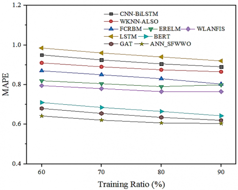
This evaluation manifest that similar to MSE, the designed model achieved less RMSE outcome, which highlights its potential of predicting loads precisely. Finally, the MAPE performance of the developed model was compared with the existing models. The existing models including CNN-BiLSTM, WKNN-ALSO, FCRBM, ERELM, WLANFIS, LSTM, BERT and GAT incurred MAPE of 0.95, 0.91, 0.87, 0.82, 0.795, 0.985, 0.71, and 0.68, respectively, while the presented algorithm earned comparatively lower MAPE of 0.642 for 60% training ratio.
These results unequivocally demonstrate that ANN_SFWWO is a superior approach for load forecasting in smart grids, consistently outperforming other methods across various metrics and training data percentages. Its exceptional performance is evident in its lower MSE, RMSE, and MAPE values, indicating a higher degree of accuracy and robustness. The ANN_SFWWO model ability to effectively learn and generalize from the training data enables it to make precise predictions, even with varying training data percentages. This is particularly crucial in smart grids, where accurate load forecasting is essential for efficient energy management, grid stability, and renewable energy integration. Furthermore, the ANN_SFWWO model adaptability to different training data percentages makes it an ideal choice for real-world applications, where data availability and quality may vary. Overall, the results unequivocally establish ANN_SFWWO as a cutting-edge approach for load forecasting in smart grids, offering a reliable and accurate solution for energy professionals and researchers alike. Its potential to optimize energy distribution, reduce energy waste, and promote sustainable energy practices makes it an invaluable tool in the pursuit of a high-performance renewable energy future.
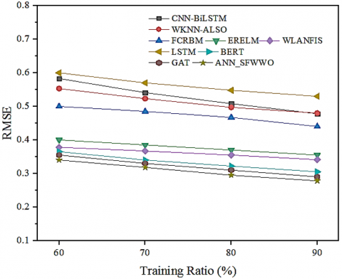
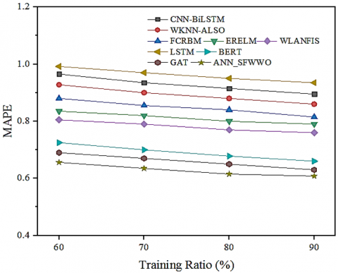
Performance comparison for D2 dataset: Figure 7 displays the comparative evaluation of system’s performances such as MSE, RMSE and MAPE with the conventional models for D2. The performances are estimated by increasing training ratios (60 to 90). For 60% training ratio, the proposed ANN_SFWWO and the conventional algorithms such as CNN-BiLSTM, WKNN-ALSO, FCRBM, ERELM, WLANFIS, LSTM, BERT and GAT obtained 0.128, 0.525, 0.307, 0.25, 0.16, 0.149, 0.33, 0.136, and 0.133, respectively. Similarly, MSE was determined for other training ratios 70, 80 and 90, as depicted in Figure 7(a). Consequently, RMSE metric was estimated and compared with existing forecasting models, as displayed in Figure 7(b). For 60% training ratio, the above-mentioned conventional models and the proposed framework earned RMSE of 0.553, 0.5, 0.4, 0.378, 0.6, 0.365, 0.355, and 0.34, respectively. This evaluation manifest that similar to MSE, the designed model achieved less RMSE outcome, which highlights its potential of predicting loads precisely. Finally, the MAPE performance of the developed model was compared with the existing models. The existing models including CNN-BiLSTM, WKNN-ALSO, FCRBM, ERELM, WLANFIS, LSTM, BERT and GAT incurred MAPE of 0.95, 0.91, 0.87, 0.82, 0.795, 0.985, 0.71, and 0.68, respectively, while the presented algorithm earned comparatively lower MAPE of 0.642 for 60% training ratio.
Figure 7. Comparative evaluation (a) MSE, (b) RMSE, (c) MAPE
These results unequivocally establish ANN_SFWWO as a pioneering approach in load forecasting, showcasing its exceptional ability to adapt and generalize across diverse datasets and training data percentages. The consistent superiority of ANN_SFWWO across various metrics, including MSE, RMSE, and MAPE with D2, demonstrates its robustness and reliability in predicting load demands. This is particularly crucial in smart grids, where accurate load forecasting enables efficient energy management, grid stability, and seamless integration of renewable energy sources. The outperformance of ANN_SFWWO across different training data percentages highlights its ability to learn and generalize from limited data, making it an attractive solution for real-world applications where data availability may be constrained. Furthermore, its consistent performance across various metrics underscores its potential to drive accurate and reliable load forecasting, enabling utilities and grid operators to make informed decisions and optimize energy distribution. The results also suggest that ANN_SFWWO can effectively handle complex load patterns and variability, making it an ideal choice for smart grids with diverse energy sources and consumption profiles. As the energy landscape continues to evolve, the ability of ANN_SFWWO to adapt and generalize across different datasets and scenarios makes it a valuable tool for ensuring grid stability and reliability. Overall, the results solidify ANN_SFWWO position as a leading approach in load forecasting, paving the way for its adoption in smart grids and contributing to a more sustainable and efficient energy future.
5.5.1 Comparison with optimization algorithms
In this module, the performances of the developed SFWWO were compared with traditional optimization models such as PSO, GA, SFOA and WWO. The metrics used in comparative analysis is convergence speed, convergence time and total computational time.
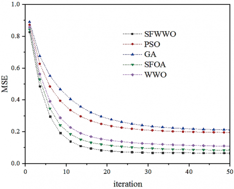
Figure 8. Convergence speed analysis
Figure 8 presents the comparison of the convergence speed of different optimization models. The convergence graph evaluates how fast the optimization models achieve their objective function. In the proposed work, the objective function is to reduce the MSE of the ANN by fine-tuning its hyperparameters to an optimal value. This extensive assessment of convergence speed demonstrates that compared to traditional algorithms, including PSO, GA, SFOA, and WWO algorithms, the designed SFWWO achieved faster and smoother convergence. It takes a smaller number of iterations to reach the optimal solution, highlighting its effectiveness in reducing error with fewer computational resources.
Table 3 tabulates the comparative assessment of different optimization models. The designed SFWWO take just 34 iterations for achieving the optimal solution, while the existing algorithms consumed comparatively more iterations. Similarly, the table illustrates the time consumed the models for reaching the optimal solution. The proposed method consumed 8.1s, while other models like PSO, GA, WWO, and SFOA consumed 8.1s, 9.6s, 8.1s, and 7.6s, respectively. This assessment validates that the designed model reaches the optimal solutions faster compared to traditional optimization models.
Table 3. Comparison of optimization models
|
Optimization Model |
No. of Iterations |
Convergence Time (s) |
Total Runtime (s) |
|
PSO |
45 |
8.9 |
12.4 |
|
GA |
50 |
9.6 |
13 |
|
WWO |
43 |
8.1 |
12.2 |
|
SFOA |
40 |
7.6 |
10.7 |
|
SFWWO |
34 |
6.5 |
9.2 |
5.6 Computational complexity analysis
To assess the practicality and feasibility of our proposed SFWWO algorithm, we conducted a comprehensive computational complexity evaluation. The experimental setup utilized an Intel i3 processor with 2 GB RAM to simulate a resource-constrained environment. The convergence analysis demonstrated that SFWWO achieves stable solutions within approximately 45–55 iterations, with the mean convergence observed at 50 iterations. Compared to PSO and GA, SFWWO exhibited faster convergence rates and consistently lower runtime per iteration, averaging approximately 1.17 seconds per iteration versus 3.21 seconds (PSO) and 4.05 seconds (GA), as detailed in Table 3 and Figure 8. Memory consumption remained consistently below 700 MB during training, making the model suitable for deployment in low-resource environments or edge devices. These results highlight SFWWO’s efficiency and practical feasibility for real-time smart grid applications.
5.7 Interpretability analysis using SHAP
Ensuring transparency in smart grid forecasting is crucial for practical decision-making. To enhance the interpretability of our ANN model, we applied SHapley Additive exPlanations (SHAP) analysis. SHAP provides feature importance scores that help identify how each input contributes to prediction outcomes. Table 4 presents a comparative evaluation of the proposed ANN_SFWWO model against several existing methods across two datasets (D1 and D2) using RMSE, MSE, and MAPE as performance metrics. Across both datasets, ANN_SFWWO consistently achieves the lowest RMSE and MSE values, indicating superior prediction accuracy and minimal error magnitude. Specifically, for D1, it records the lowest RMSE (0.28) and MSE (0.07), outperforming advanced models like BERT and GAT. In D2, it maintains this trend with an RMSE of 0.225 and MSE of 0.04. Although its MAPE in D2 (0.77) is marginally higher than GAT (0.76) and BERT (0.765), the overall performance confirms the robustness and generalizability of ANN_SFWWO. This highlights the effectiveness of its hybrid structure and optimization strategy over conventional and deep learning models.
The SHAP analysis revealed that increases in solar irradiance and temperature strongly correlated with higher predicted load, while wind speed exhibited a complex nonlinear relationship. This visual interpretability helps grid operators intuitively understand the forecasting logic, increasing their trust in the predictive outcomes. Consequently, applying SHAP significantly enhances the practical utility of our model by providing clear explanations for each prediction, vital for informed operational decisions in smart grids.
Table 4. Comparative discussion of ANN_SFWWO
|
Datasets |
Metrics |
CNN-BiLSTM |
WKNN-ALSO |
FCRBM |
ERELM |
WLANFIS |
LSTM |
BERT |
GAT |
Proposed ANN_SFWWO |
|
D1 |
RMSE |
0.5 |
0.449 |
0.37 |
0.31 |
0.3 |
0.46 |
0.295 |
0.288 |
0.28 |
|
MSE |
0.269 |
0.2 |
0.14 |
0.1 |
0.091 |
0.215 |
0.088 |
0.083 |
0.07 |
|
|
MAPE |
0.9 |
0.87 |
0.81 |
0.8 |
0.77 |
0.82 |
0.74 |
0.73 |
0.61 |
|
|
D2 |
RMSE |
0.93 |
0.72 |
0.35 |
0.275 |
0.255 |
0.69 |
0.242 |
0.239 |
0.225 |
|
MSE |
0.88 |
0.53 |
0.12 |
0.07 |
0.06 |
0.54 |
0.059 |
0.057 |
0.04 |
|
|
MAPE |
0.91 |
0.9 |
0.84 |
0.8 |
0.797 |
0.85 |
0.765 |
0.76 |
0.77 |
5.8 Discussion
This study worked on developing a hybrid algorithm for load forecasting in smart grids. The novelty of the model lies in the efficient integration of optimization potential of hybrid SFWWO into ANN. The ANN algorithm captures the complex pattern and hierarchical feature representations within the historical data for forecasting loads in future scenarios, while SFWWO algorithm fine-tunes the ANN hyperparameters continuously over iterations, improving its training speed, and enhancing prediction accuracy. The designed model was validated using two public grid datasets and the results are assessed under different scenarios for highlighting the system’s efficiency in load prediction.
The comparative analysis in Table 3 demonstrates the superiority of ANN_SFWWO in load forecasting for smart grids, surpassing other approaches in terms of RMSE, MSE, and MAPE values. The exceptional performance of ANN_SFWWO can be attributed to its efficient feature selection procedure, which enables it to handle diverse training data with remarkable resilience. By identifying and utilizing the most relevant features, ANN_SFWWO enhances model correctness, resulting in an impressive MSE value of 0.040 in Dataset 2. Moreover, ANN_SFWWO outperforms alternative strategies that employ feature extraction techniques to improve model performance, achieving a lower RMSE value of 0.225. This highlights the effectiveness of ANN_SFWWO's optimization procedure in training the ANN, enabling it to adapt and learn from data. The optimal MAPE solution of 0.770 further underscores ANN_SFWWO's potential for smart grid load forecasting. In contrast, higher error levels in alternative approaches indicate their limited accuracy and robustness. The superior performance of ANN_SFWWO across various metrics and datasets emphasizes its potential to drive accurate and reliable load forecasting in smart grids. As the energy landscape continues to evolve, the adaptability and learning capabilities of ANN_SFWWO make it an attractive solution for ensuring grid stability and reliability. The comparative discussion highlights the significance of efficient feature selection and optimization procedures in enhancing model performance. The results suggest that ANN_SFWWO approach can be applied to various smart grid applications, enabling utilities and grid operators to make informed decisions and optimize energy distribution.
5.8.1 Limitations
Although proposed ANN_SFWWO framework offered strong performance in load forecasting, there are several limitations that need to be resolved. Firstly, it lacks interpretability as it doesn’t highlight the constraints which influences load pattern. This limits its applicability in real-time scenarios where transparent decision-making is need for effective functioning of smart grid. Secondly, the tuning of parameters using SFWWO is sensitive to initial conditions. It makes the system works well on pre-defined scenarios but cannot generalize well on other cases. Thirdly, the presented model was validated on only two datasets and it is not validated across diverse grid conditions, which limits its scalability. In addition, the presented method cannot examine the temporal dependencies within the data, which degrades its performances under changing geographic conditions. Finally, the presented study lacks implementation or testing on real-time environment, which is significant for evaluating its applicability in real-world applications.
This study presents an advanced signal processing-driven approach for load forecasting in smart grids, utilizing ANN optimized by SFWWO. By incorporating feature selection via Ruzicka and Motyka similarity metrics and refining classification through Dice coefficient-based fusion, the proposed model enhances predictive accuracy and robustness. Comparative analysis with existing methods demonstrates the superiority of ANN_SFWWO, achieving the lowest RMSE and MSE values.
The results emphasize the critical role of signal processing in refining smart grid forecasting methodologies. Future research will explore real-time implementation strategies to improve scalability and integration with emerging AI-driven smart grid technologies. The future work should incorporate Graph Neural Networks (GNNs) or attention mechanisms to capture the spatial and temporal dependencies present in load data, for improving forecasting accuracy.
[1] Abu-Salih, B., Wongthongtham, P., Morrison, G., Coutinho, K., Al-Okaily, M., Huneiti, A. (2022). Short-term renewable energy consumption and generation forecasting: A case study of Western Australia. Heliyon, 8(3): e09152. https://doi.org/10.1016/j.heliyon.2022.e09152
[2] Javaid, N., Hafeez, G., Iqbal, S., Alrajeh, N., Alabed, M.S., Guizani, M. (2018). Energy efficient integration of renewable energy sources in the smart grid for demand side management. IEEE Access, 6: 77077-77096. https://doi.org/10.1109/ACCESS.2018.2866461
[3] Tarmanini, C., Sarma, N., Gezegin, C., Ozgonenel, O. (2023). Short term load forecasting based on ARIMA and ANN approaches. Energy Reports, 9(Supl3): 550-557. https://doi.org/10.1016/j.egyr.2023.01.060
[4] Abumohsen, M., Owda, A.Y., Owda, M. (2023). Electrical load forecasting using LSTM, GRU, and RNN algorithms. Energies, 16(5): 2283. https://doi.org/10.3390/en16052283
[5] Saleh, A.I., Rabie, A.H., Abo-Al-Ez, K.M. (2016). A data mining based load forecasting strategy for smart electrical grids. Advanced Engineering Informatics, 30(3): 422-448. https://doi.org/10.1016/j.aei.2016.05.005
[6] Zhang, D., Jin, X., Shi, P., Chew, X. (2023). Real-time load forecasting model for the smart grid using Bayesian optimized CNN-BiLSTM. Frontiers in Energy Research, 11: 1193662. https://doi.org/10.3389/fenrg.2023.1193662
[7] Rabie, A.H., I Saleh, A., Elkhalik, S.H.A., Takieldeen, A.E. (2024). An optimum load forecasting strategy (OLFS) for smart grids based on artificial intelligence. Technologies, 12(2): 19. https://doi.org/10.3390/technologies12020019
[8] Wen, X., Liao, J., Niu, Q., Shen, N. Bao, Y. (2024). Deep learning-driven hybrid model for short-term load forecasting and smart grid information management. Scientific Reports, 14(1): 13720. https://doi.org/10.1038/s41598-024-63262-x
[9] Hafeez, G., Alimgeer, K.S., Khan, I. (2020). Electric load forecasting based on deep learning and optimized by heuristic algorithm in smart grid. Applied Energy, 269: 114915. https://doi.org/10.1016/j.apenergy.2020.114915
[10] Aly, H.H. (2020). A proposed intelligent short-term load forecasting hybrid models of ANN, WNN and KF based on clustering techniques for smart grid. Electric Power Systems Research, 182: 106191. https://doi.org/10.1016/j.epsr.2019.106191
[11] Ali, M., Adnan, M., Tariq, M., Poor, H.V. (2020). Load forecasting through estimated parametrized based fuzzy inference system in smart grids. IEEE Transactions on Fuzzy Systems, 29(1): 156-165. https://doi.org/10.1109/TFUZZ.2020.2986982
[12] Naz, A., Javed, M.U., Javaid, N., Saba, T., Alhussein, M., Aurangzeb, K. (2019). Short-term electric load and price forecasting using enhanced extreme learning machine optimization in smart grids. Energies, 12(5): 866. https://doi.org/10.3390/en12050866
[13] Dai, Y., Zhao, P. (2020). A hybrid load forecasting model based on support vector machine with intelligent methods for feature selection and parameter optimization. Applied Energy, 279: 115332. https://doi.org/10.1016/j.apenergy.2020.115332
[14] Technical indicators. https://www.tradingtechnologies.com/xtrader-help/x-study/technical-indicator-definitions/list-of-technical-indicators/, accessed on Aug. 1, 2024.
[15] Umamaheswari, G.R., Kalamani, D. (2015). Monthly groundwater level fluctuation prediction using artificial neural network. International Journal of Applied Engineering Research, 10(11): 29937-29948.
[16] Sattar, D., Salim, R. (2021). A smart metaheuristic algorithm for solving engineering problems. Engineering with Computers, 37(3): 2389-2417. https://doi.org/10.1007/s00366-020-00951-x
[17] Zheng, Y.J. (2015). Water wave optimization: A new nature-inspired metaheuristic. Computers & Operations Research, 55: 1-11. https://doi.org/10.1016/j.cor.2014.10.008
[18] Zhang, Z. (2024). Deep analysis of time series data for smart grid startup strategies: A transformer-LSTM-PSO model approach. arXiv preprint arXiv:2408.12129. https://doi.org/10.48550/arXiv.2408.12129
[19] Kumari, S., Kumar, N., Rana, P.S. (2021). Big data analytics for energy consumption prediction in smart grid using genetic algorithm and long short term memory. Computing & Informatics, 40(1): 29-56.
[20] Hasanat, S.M., Younis, R., Alahmari, S., Ejaz, M.T., Haris, M., Yousaf, H., Watara, S., Ullah, K., Ullah, Z. (2024). Enhancing load forecasting accuracy in smart grids: A novel parallel multichannel network approach using 1D CNN and Bi-LSTM models. International Journal of Energy Research, 2024(1): 2403847. https://doi.org/10.1155/2024/2403847
[21] Mounir, N., Ouadi, H., Jrhilifa, I. (2023). Short-term electric load forecasting using an EMD-BI-LSTM approach for smart grid energy management system. Energy and Buildings, 288: 113022. https://doi.org/10.1016/j.enbuild.2023.113022
[22] Tao, P., Ma, H., Li, C., Liu, L. (2023). Intelligent grid load forecasting based on BERT network model in low-carbon economy. Frontiers in Energy Research, 11: 1197024. https://doi.org/10.3389/fenrg.2023.1197024
[23] Peng, B. (2024). The application of visibility graph and graph attention network for urban smart grid short-term load forecasting. https://doi.org/10.11159/icert24.111