Tanvir Fatima Naik Bukht![]() | Naif S. Alshassabi | Haifa F. Alhasson | Bayan Alabdullah | Ahmad Jalal*
| Naif S. Alshassabi | Haifa F. Alhasson | Bayan Alabdullah | Ahmad Jalal*![]()
© 2025 The authors. This article is published by IIETA and is licensed under the CC BY 4.0 license (http://creativecommons.org/licenses/by/4.0/).
OPEN ACCESS
Human Activity Recognition (HAR) is crucial to intelligent smart home systems. In this research, we propose a novel skeleton-based method for recognizing human activities accurately. Gamma correction is applied as a preprocessing step to improve image quality. Then, we use a robust combination of Multiple Object Tracking (MOT) and graph-based segmentation techniques to extract precise human silhouettes from video sequences. This research also introduces a novel innovation in developing a 23-joint skeleton model that accurately identifies and tracks key body joints. A comprehensive set of features extracted from this skeleton data is derived, including relative joint angles, joint proximity measures, joint stability, and full body features, which are extracted using BRIEF, LATCH, and MSER. A fuzzy optimization technique is employed to find the most discriminative features to optimize feature selection. Finally, a Convolutional Neural Networks (CNN) classifier is trained on the optimized features to classify human activities accurately. Experimental results demonstrate the effectiveness of our approach, with ShakeFive2 achieving an 88% accuracy rate and BIT-Interaction achieving 94% on a benchmark dataset. This work contributes to advancing human activity understanding in various domains, such as surveillance, human-behavior interaction, healthcare, sports, and social robotics.
daily living activities recognition, machine learning, behavior recognition, multimodal data, patient monitoring, smart homes, body pose, deep learning
HAR is a central problem in computer vision that has wide interests in health care, human-computer interaction [1], surveillance, and social robotics. Correct perception of human activities would allow systems to read social gestures, anticipate behavior, and achieve intuitive human-machine interaction. Nevertheless, HAR is a very difficult task because of the complexities in human behaviour, variation in pose, lighting conditions, and occlusion [2]. Current HAR approaches usually use handcrafted features or deep learning-based methods. Moreover, handcrafted features may be sensitive to the pose and lighting variations.
Information, particularly RGB images that the cameras [3] capture, multifaceted and varied [4], offers a chance to expose numerous hidden patterns of how people act in the setting of smart homes. Thus, based on this information and developing a specialized Skeleton model, the proposed study aims to increase the state of art in HAR and offer a more detailed and accurate way of understanding and engaging with human activities that are applicable in the context of smart homes. In turn, the main contribution of the proposed research is the enhancement of the creation of smart environment technologies through the enhancement of the capacity of HAR through a sophisticated and dedicated data analysis model. This paper aims not only to inspire the database of current HAR studies but also to create a foundation for developing more adaptive systems of smart home environments that would take into account the inhabitants' preferences in their occupancy patterns most efficiently.
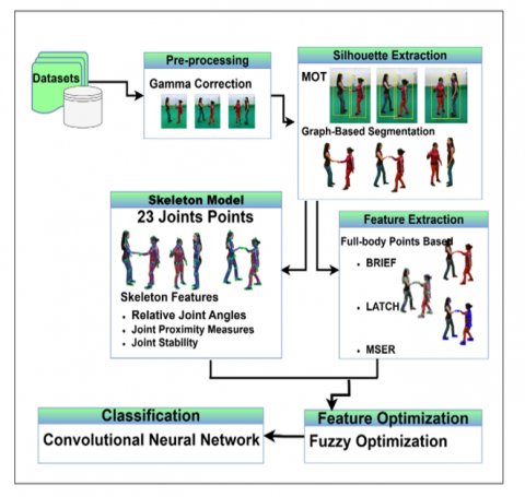
In order to overcome these issues, this paper suggests a new HAR framework that integrates pre-processing, silhouette extraction, feature extraction, and fuzzy optimization-based machine learning classification. Our method seeks to learn discriminative features, but with computational efficiency and invariance to changes in the image data. This research addresses some of these challenges by developing a novel approach combining advanced image processing techniques, innovative feature extraction methods, and powerful machine learning algorithms. Our proposed system consists of five key stages:
(1) Pre-processing using gamma correction to enhance video quality and handle varying illumination conditions.
(2) Silhouette extraction employing both motion-oriented tracking (MOT) and graph-based segmentation techniques.
(3) Novel skeleton model and feature extraction include relative joint angles, joint proximity measures, and joint stability.
(4) Full body Feature extraction combining BRIEF descriptors with a novel set of 23 key joint points.
(5) Fuzzy optimization to refine extracted features.
The paper is structured as follows: a review of the literature on the studies related to HIR is provided in Section II. Section III gives the HAR proposal scheme that is made up of pre-processing phase, silhouette extraction, feature extraction phase, fuzzy optimization phase, and the classification phase. Section IV is devoted to experimental findings and assessments. Finally, section V presents the conclusion and recommends further studies.
This section provides an extensive literature review on both conventional and modern ML-based techniques for HIR recognition in smart environments. To make it easier for the reader to follow, we have broken down the literature review into two categories: Traditional machine learning approaches and Deep machine-learning methods.
2.1 Traditional machine learning methods for HAR
Traditional ML techniques have been extensively employed in human activity recognition, offering a foundation for understanding and addressing the complexities of social behavior analysis. One of the earliest and most influential methods was the Hidden Markov Model (HMM). HMMs were widely used for action recognition and gesture analysis, demonstrating the power of probabilistic models in capturing sequential dependencies in human motion. However, there were restrictions on using HMMs, such as the problems that occurred when modelling human interactions as they have variable patterns, while the HMM approaches depended on state-transition models.
Support Vector Machines (SVMs) were another major contribution towards the field made by them. In generalization capabilities and handling high-dimensional feature space, SVM benefits have been identified when focusing on differentiating between various forms of human activity based on extracted features [5]. Despite that, SVMs were efficient, needed substantial preprocessing of input features, and could sometimes fail on real-world differences such as occlusions or variable lighting conditions [6]. Other emphasized machine learning techniques included Decision Trees and Random Forests that formed part of earlier strategies in human activity recognition. These ensemble methods provided better resistance to noise and outliers than individual decision trees, though they were most suitable for capturing human activity hierarchies. While Decision Trees were relatively easy to interpret the decision-making process, Random Forests gave better generality. However, both methods mainly suffered from poor generalization performance on new, unseen behaviors and were unsuitable for social scenarios.
Naive Bayes classifiers were also included in the traditional machine-learning methods for human activity recognition. They were able to give accurate results that are easy to understand and apply in real-time situations. The Naive Bayes models assumed that each feature was independent, so it sometimes overfitted some problems, but it was still a good model for its simplicity. Working with large amounts of data was easy for them, but their approach was not as effective when the data was more detailed and could not be separated linearly [7].
SVM and KNN were also two mainstream approaches used in human activity recognition. As it was highlighted, KNN provides a greater liberty in choosing the number of neighbours k and the distance measures so that it could be adapted to operation on diverse data and contexts. It was favored by researchers and practitioners since it is easy to apply and implement. But the performance of KNN may strongly rely on the quality of data we use as samples, and it may lead to the discrepancy of the results when the same algorithm is executed repeatedly [8].
2.2 Advance machine learning methods for HAR
Spatial Temporal Graph Convolutional Networks (ST-GCN) introduced by Zahoor and Jalal [9], model the human skeleton as a graph, capturing both spatial and temporal dynamics for improved accuracy. Rahevar et al. [10] enhanced graph convolutions with attention mechanisms to dynamically weigh joints and frames based on their importance. Transformer-based models have recently gained traction [11], effectively modeling long-range temporal dependencies in skeleton sequences with self-attention mechanisms. Tayyab and Jalal [12] also demonstrated that fusing skeleton and RGB data modalities enhances recognition robustness, particularly in challenging environments such as occlusions or variable lighting.
Challenges associated with the subject of human activity recognition have led to the emergence of new forms of machine learning. One such improvement is the use of the well-developed Gaussian Mixture Models (GMMs), which give a reasonable chance of separating these motion patterns based on the complexity of their distributions. It seems that GMMs were especially useful in tracking one more or less simultaneous movement and capturing the true character of human motion, making highlighting slight changes in behaviour possible [13]. However, GMMs were sensitive to initializations and often had issues with ‘mode-seeking’, especially in high-dimensional feature space.
Kernel Fisher Discriminant Analysis (KFDA) and other Kernel-based methods have been used for human activity classification. It demonstrated that KFDA could distinguish between similar and different actions and build useful features from raw motion data for recognizing real PAM [14]. Since it wasn’t designed to process only linearly separable data, which was a perfect fit for capturing the complexity of human behavior. However, KFDA incorporated strict prior choices for the kernel functions and hyperparameters, which could be cumbersome.
XGBoost, which has recently attracted much attention as a gradient-boosting technique, is acknowledged for its superior performance and understanding. Different machine learning activities, such as human activity recognition, have recorded high proficiency and sustainability by applying XGBoost [15]. This is particularly advantageous in dealing with big data and modelling higher-order interactions of variables as actions. Evaluation of XGBoost in HAD and its Applications: XGBoost has been used to demonstrate success in extracting the discriminant features of motion data and classifying complicated social actions [16]. Another great strength of using XGBoost is identifying feature importance scores that allow for interpretation. These scores give the idea as to which of the features make the most crucial impact on the model, which would help the researcher explain the mechanisms behind human activity recognition. Such interpretability is particularly important in areas such as human-computer interaction since knowledge of how an AI system came to its particular decision might help to optimize the latter’s functioning.
Our approach to human activity recognition includes five stages that help overcome crucial difficulties in the domain of social behavior analysis. Hence, we propose a novel system that performs several steps in recognising different human activities, including applying enhanced image processing algorithms, using sophisticated features extraction techniques, and employing state-of-the-art machine learning algorithms. A brief overview of the architecture of HAR has been provided in Figure 1. Subsections below elaborate on each of these layers in this HA recognition architecture.
Figure 1. The architecture diagram of purposed system for HAR
3.1 Data preprocessing
To implement all the analytical and computational algorithms in the present work, all the video frames should be divided into different images. Gamma correction is then performed on these frames to minimize noise. This process blurs the background, smooths the image, and makes the human subject stand out more visibly. This step is significant for the accuracy and efficiency of the proposed system.
Gamma correction is typically applied to images to begin to make the images appear more uniformly natural to the human eye [17]. Contrast sensitivity is nonlinear, which means that our ability to see changes in brightness is different in light and dark surfaces. Gamma correction helps correct the nonlinear contrast and gamma curves, making the image seem more natural. To do this, gamma correction applies a mathematical computation to alter each pixel’s brightness level. The adjustment quantity is regulated by a number referred to as the gamma value. Gamma’s value of greater than 1 makes the image darker, and where the value is less than 1 the image becomes brighter. With the help of gamma correction, the quality of the images can be enhanced, and the primary parameter determining the final image is easier to understand. The equation for gamma correction is given below, and the result is shown in Figure 2 and Eq. (1):
$X_{\text {out }}=X_{\text {in }}^\gamma$ (1)
A separate Gamma correction is applied to every video frame so the image appears natural. The extent of correction applied depends on the general brightness of scenes encountered in a video. This is because the adaptive approach ensures that bright and black portions of the image receive the right measure signal to get a better image that can be processed further.
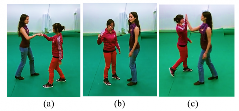
Figure 2. Gamma correction is applied for reduce noise (a) fist-bump (b) explain (c) high five
3.1.1 Silhouette extraction
Silhouette extraction also plays an essential role in other computer vision problems such as object recognition, tracking, and segmentation. For instance, accurately extracting sufficient human silhouettes is considered a challenging task in feature extraction. Here, we are postulating how to pinpoint the shapes of people. Putting the silhouette in place is critically important to extracting and detecting the right features.
3.1.2 Multiple Object Tracking (MOT)
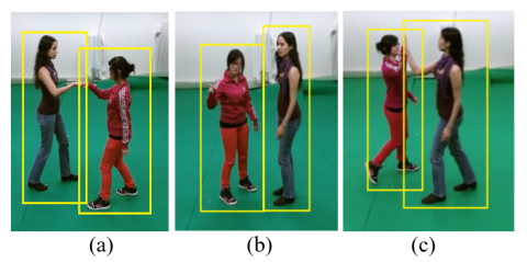
MOT is intended to track a set of objects in an image sequence. MOT is applied in various systems, including security, automated driving, and video analysis [18]. The main goal of MOT is to identify objects with high accuracy and maintain their identity while predicting their future position [19].
Figure 3. Silhouette extraction results of MOT (a) fist-bump (b) explain (c) high five
This process has some challenges, such as occlusions, image variation, and frequently interacting objects. In order to handle these difficulties, MOT algorithms use different methods, e.g., data association, motion prediction, and object representation. The first is using the object tracking methods, which involve using an object detector to detect objects in each frame and then link these detections across frames to get tracks. The MOT results are depicted in Figure 3.
3.2 Graph-based segmentation (GBS)
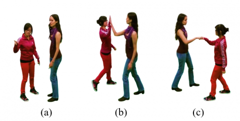
GBS is a powerful image-processing technique that uses graph theory to divide image into meaningful regions [20]. The idea here is to represent each of the pixels in the image as a node in a graph, and the edges between nodes indicate pixel similarity. We seek to segment the image into distinct regions via the minimal total weight of edges that must be cut. This is especially useful for silhouette segmentation, where the goal is distinguishing the foreground object from the background. Graph partitioning can be applied to such a graph where the nodes are pixels and edges represent pixel similarities to segment precisely.
The main advantage of graph-based segmentation lies in its flexibility in coping with complex image structures and varying color textures. Second, the segmentation process defines the weights of the edges based on similarities between the pixels. An algorithm like normalized cuts or spectral clustering is used to partition the constructed graph into disjoint regions. These algorithms aim to minimize the weights of the edges between segments so that the intersected segments are both meaningful and precise. This approach improves the general accuracy and efficiency of the segmentation process while providing better clarity of the segmented silhouette.
$\operatorname{Cut}(G, H)=\sum_{u \in G, v \in H} w e(u, v)$ (2)
Eq. (2) calculates the total weight of the edges that must be cut to separate the graph into two disjoint sets (G) and (H). (G) and (H) are two sets of nodes (pixels) in the graph. This notation means that (u) is a node in set (G) and (v) is a node in set (G). we(u, v) represents the weight of the edge between nodes (u) and (v). Figure 4 shows the result of graph-based segmentation.
Figure 4. Graph-based segmentation (a) fist-bump (b) explain (c) high five
3.3 Extraction of feature
This is a critical step in our pipeline, where we combine the Binary Robust Invariant Features (BFIRE) descriptor with a novel set of 23 key joint points features. This hybrid approach aims to capture both local texture information and global structural properties of human movements.
3.3.1 Binary robust invariant features (BRIEF)
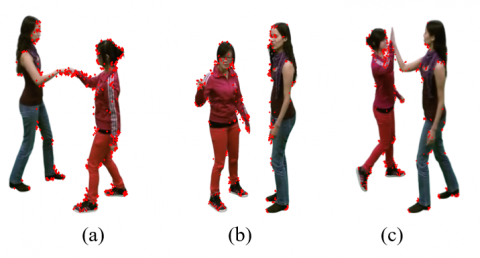
BRIEF is a feature descriptor used in a computer vision technique for image analysis. It is a fast algorithm suitable for real-time use and optimized for speed. Compared with other descriptors such as SIFT and SURF, which use float-point numbers and much computation, BRIEF utilizes binary string to express the features of the image. This binary representation makes a quick calculation and matching using the Hamming distance, which we know is faster to compute than the Euclidean distance in other methods. This is done by performing simple intensity difference tests between a pair of pixels within a smoothed image patch and an outcome in a highly discriminative and compact descriptor popularly known as the BRIEF descriptor [12]. Another advantage of the BRIEF descriptor is insensitivity to photometric and geometric distortions, such as changes of illumination and view angle. This is especially the case where the algorithms' performance and the rate of computation matter, most notably in mobile and embedded systems.
Figure 5. BRIEF results (a) fist-bump (b) explain (c) high five
$\operatorname{BRIEF}(p)=\sum_{i=1}^n 2^{i-1} \cdot\left(I\left(p+\Delta x_i\right)<I\left(p+\Delta y_i\right)\right)$ (3)
In Eq. (3), BRIEF(p), (I)=Intensity of image at a given point (p), Δxi=First pixel pair, and Δyi=Second pixel pair is predefined. The end product is a set of binary numbers that can be translated into the BRIEF descriptor, as seen in Figure 5. BRIEF is a fast feature detector, but is sensitive to scale variations, rotation, and viewpoint changes. This can cause the system to struggle when objects are hidden or when the viewpoint changes a lot, resulting in some features being blocked.
3.3.2 Learned arrangements of three patch codes (LATCH)
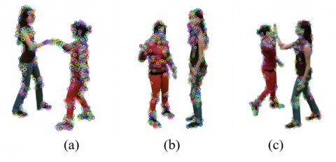
LATCH has thus surfaced as the central enabler for HAR and behaviour analysis. Using LATCH for feature extraction, a reliable approach is built to precisely recognise complex movements and gestures in smart contexts. In addition to enhancing the analysis of data it also makes a major contribution to the optimization and accuracy of the behavioral observation systems in different environments. Incorporating LATCH in the design of image-based systems provides an improved solution, especially for HAR in smart home settings. In addition to enhancing the performance of measures of accuracy, this feature extraction approach also opens greater avenues for the development of behavior recognition systems and for understanding the ways in which people interact within smart homes, thus improving the general acceptance of these technologies as part of people’s daily lives.
Further, merging the application of image technologies with the feature extraction form of LATCH, offer a revolutionized approach in smart home-related studies. This is because breaking down human activities and behaviors into their essentials provides great room for changing the face of image applications in various fields. Integrating data analysis and LATCH-based feature extraction accelerates trends in advancing behavior recognition systems’ accuracy and robustness and paves the way for developing intelligent sensing solutions for the new generation that reflect the dynamic living environment requirements in contemporary society.
$L(f)=\sum_{i=1}^n \sum_{i=1}^n \sqrt{| | f(i)-\left.f(j)\right|_2 ^2}$ (4)
In Eq. (4), L(f) is the LATCH descriptor calculation, and f(j) and f(i) are representations of feature vectors of the i th and j th patch in the image, respectively. The function L(f) considers the distances between all pixel feature vector pairs in the patch; such distances provide invaluable information about the spatial context that is fundamental for feature extraction.
$h(f)=\frac{1}{n} \sum_{i=1}^n f(i)$ (5)
The computation of the mean feature vector h(f) of an image patch is given in Eq. (5) h(f), which for instance, to total number of feature vectors inside the patch, is denoted by n. This equation aids in extracting representative descriptor by averaging the individual feature vectors so that we end up with salient features that encapsulate the characteristics of a patch for robust feature representation for further analysis and Results shown in Figure 6.
Figure 6. LATCH results (a) fist-bump (b) explain (c) high five
LATCH offers improved robustness by incorporating texture and color information. Yet, it may not work well when the background is messy, as it becomes unclear which patches belong together or when there is not enough light, making it hard to tell apart the local textures.
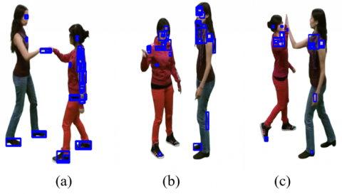
3.3.3 Maximally stable extremal regions (MSER)
The entity can be accurately recognised so that smart homes and image technologies work seamlessly in the realm of recognizing human activities. In this work, we leverage advanced computer vision techniques to extract features from data streams using MSER as a means to discern complex human activities in the smart home scenario. Our study exploits MSER regions’ stability and distinctiveness to improve HAR system performance, encouraging the development of smarter and more responsive smart home environments.
Utilizing MSER to extract salient features from data, the proposed methodology allows the characterization of different human activities in smart home contexts. Our approach attempts to capture meaningful patterns and dynamics associated with different activities (performed by occupants) by identifying stable extremal regions over readings. Additionally, the incorporation of MSER feature extraction into existing networks provides a unique framework for real time action recognition and rapid, context-consistent action elicitation in smart homes from human hand gestures and behaviors.
$R(p)=\frac{\left\{E\left(I^{\{p\}}\right)\right\}}{\left\{E\left(I^{\{p-1\}}\right)\right\}}$ (6)
The stability measure of the extremal region at time p is denoted by R(p) and can be defined in Eq. (6) as, R(p) = Intensity of extremal region at time p/Intensity of extremal region at time (p-1). This measure helps quantify and define the stability and importance of MSER regions within subsequence data frames.
These features encapsulate the distinctive characteristics of extremal regions in data, providing valuable cues for HAR in smart home applications and results shown in Figure 7.
Figure 7. MSER results (a) fist-bump (b) explain (c) high five
MSER excels at detecting stable regions but is sensitive to noise and illumination variations. In low-light conditions, when the light is low, MSER may not find stable regions and in cases of occlusion, the regions of interest can become divided or disappear, leading to inconsistency in extracting features.
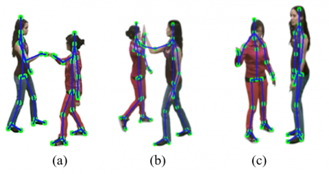
3.4 Skeleton model
The skeletal geometry features are very useful when the information is obtained from the structure of skeletal [21] to determine human behavior and motion [22]. Algorithm 1 demonstrate that the output of our proposed skeleton mode needs to be tophead (TH), neck, right-shoulder (RS), right-elbow (RE), right-wrist (Rw), right-hand (Rh), Left-Shoulder (LS), Left-Elbow (LE), Left-Wrist (LW), Left-hand (Lh), Pelvis, Right-Hip, Right-Knee, Right-Ankle, Right-foot, Right-heel, Left-Hip. The qualities are the spatial arrangements and to the geometry of the most important points of the human skeleton such as locating joint, length of bones, R is used for right and L is used for left. A widely used approach to extract skeleton geometry features is by calculating the Euclidean distances between pairs of skeleton joints. The results provide clues for human poses and movements by distance calculations of the joints in some combinations.
$d_{l m}=\sqrt{\left(a_l-a_m\right)^2+\left(s_l-s_m\right)^2+\left(d_l-d_m\right)^2}$ (7)
In Eq. (7), $d_{l m}$ is indeed the Euclidean distance between the $l^{\{t h\}}$ and $m^{\{t h\}}$ joints of the skeleton. The coordinates of the $l^{\{t h\}}$ joint are correctly denoted as $\left(a_l, s_l, d_l\right)$, and the coordinates of the $m^{\{t h\}}$ joint as $\left(a_m, s_m, d_m\right)$. The formula calculates the distance in three dimensions by calculating the square root of the sum of the squares of the differences of the $\mathrm{a}, \mathrm{s}$ and d coordinates. The skeleton geometry features can be used to create motion capture systems which generate a great deal of information about structural and movement properties of humans. In Figure 8, the results are shown:
|
Algorithm 1: Novel SkeleTrack23 Algorithm for human activity recognition. |
|
Input: Human Silhouettes Segmented (S) Output: 23 key points of body Step 1: Extract Boundaries of Both Silhouettes L1= silhouette left boundary R1 = silhouette right boundary H = silhouette-height W = width of S B = bina-rize (S); BW = bw-boundaries(B); Object = detect-object (B, Bounding-box, Area); Step 2: For Outermost Pixels Boundaries of Both S to be Search for x= 1 to L1 for y = 1 to R1 Find (L1; R1) Pixel - Top = [max-y, x]; Pixel - Left = [y, min-x]; Right - pixel = [y, max-x]; Pixel - Left Bottom = [min-x, min-y]; Right - pixel Bottom = [max-x, min-y]; end end Step 3: Bottom, Left, Top, and Right Regions of Both Silhouettes [cols, rows] = size(Object); H = rows; W = cols; Top_half = floor(H/2); Region of Head = floor(Top/ 3); Region of Torso = half of Top - Region of Head; Step 4: Identify Hd and Neck Y-t = (H / 2); X-t = (W / 2); T_H = [Xt, Top_Pixel(2)]; Neck = [Xt, Top_Pixel(2) + (Head_Region / 2)]; Step 5: Identify Shoulders, Spine, and Pelvis R_S = [Xt + (W / 8), Neck(2) + (Torso_Region / 4)]; L_S = [Xt - (W / 8), Neck(2) + (Torso_Region / 4)]; S_T = [Xt, Neck(2)]; S_C = [Xt, Yt]; Pelvis = [Xt, (3 * Yt) / 2]; Step 6: Identify Arms and Wrists R_E = [Xt + (W / 8), Neck(2) + (Torso_Region / 2)]; R_w = [Xt + (W / 8), Neck(2) + (3 * Torso_Region / 4)]; R_h = [Xt + (W / 8), Neck(2) + Torso_Region]; L_E = [Xt - (W / 8), Neck(2) + (Torso_Region / 2)]; L_W = [Xt - (W / 8), Neck(2) + (3 * Torso_Region / 4)]; L_H = [Xt - (W / 8), Neck(2) + Torso_Region]; Step 7: Identify Legs and Feet R_Hip = [Xt + (W / 8), (3 * H) / 4]; R_Knee = [Xt + (W / 8), (7 * H) / 8]; R_Ankle = Bottom_Right_Pixel; R_Foot = Bottom_Right_Pixel; R_Heel = [Bottom_Right_Pixel(1), Bottom_Right_Pixel(2) - (H / 20)]; L_Hip = [Xt - (W / 8), (3 * H) / 4]; L _Knee = [Xt - (W / 8), (7 * H) / 8]; L _Ankle = Bottom_Left_Pixel; L _Foot = Bottom_Left_Pixel; L _Heel = [Bottom_Left_Pixel(1), Bottom_Left_Pixel(2) - (H / 20)]; return |
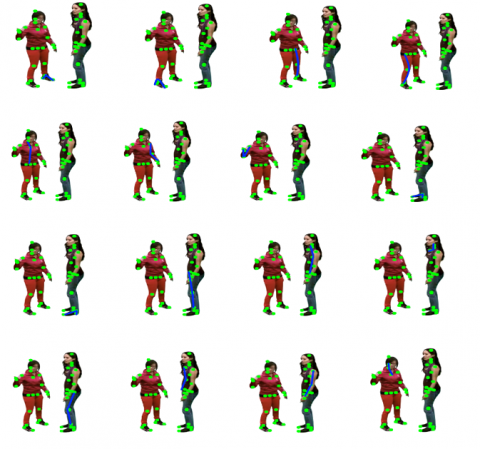
Figure 8. SkeleTrack23 results (a) fist-bump (b) explain (c) high five
When analyzing human interaction recognition using a skeleton model of 23 joint points, three key feature extraction techniques stand out: Relative Joint Angles, Joints Proximity Measures, and Joints Stability. Each of these techniques offers unique insights into human movement and interaction, particularly in the context of computer vision.
3.5 Relative joint angles
Relative joint angles are obtained by finding the angles between adjoining joints of the skeleton model. For instance, the angle between the limb shoulder and limb elbow can establish a relation with arm movements during interaction. This feature is very important in modeling human motion because it reveals the motion of body parts in reference to other parts. Under computer vision, these angles can therefore be mined from video data by employing algorithms that tend to track joint position over time. Since these angles can be measured, a precise assessment of motion can be conducted, starting from reaching or throwing, which may help solve a problem of identifying interactions between people.
In human pose estimation and modeling a human skeleton, describing the major joint points, for example, relative joint angles, is crucial to learning human movement patterns and recognizing actions. These relative joint angles are essential in understanding the spatial positioning of the various body segments with regards to other body segments to produce the movements under analysis. When using the 23 key joint points in the skeleton model, we can calculate these relative joint angles for the dynamic aspects of human movement and postures. In computing the relative joint angles, the analyst needs to think of two linked, succeeding joints joined by a bone piece on the skeletal Figure 9. One possible definition of the relative joint angle of two successive bones is to state it as the angle formed by the afroed escribed segments of the particular bones located at the particular joint. This angle gives the status of the positioning of body parts in relation to other parts thus assisting in the analysis of human gesticulation. When these relative joint angles are systematically computed for all joint pairs in the described skeleton model you obtain a complete set of features that encodes the complex spatial interactions of the human body.
Figure 9. SkeleTrack23 use for relative joint angle feature extraction
Relative joint angles are determined using mathematical algorithms that are applied on trigonometric principles and measured geometrical angles. One of these approaches is to appear the dot product of the vectors – the representations of the bone segments associated with a given joint. By applying the dot products formula, one can calculate the cosine of the relative joint angle, making it easy to measure the angular displacement of adjacent body parts. Further, there are some computational methods like inverse trigonometry where coefficients are transformed into required angle measurements in terms of degrees and radians in order analyze the quantities of joint angles and movements of the skeletal model.
In the following way where (θAB) is the angle between two joints A and B, the angle between them can be calculated by dot product of vectors constructed by two joints A and B dot product of vectors formed by these joints is as shown in Eq. (8):
Angle $\cos \left(\theta_{A B}\right)=\frac{\vec{v}_A \cdot \vec{v}_B}{\left|\vec{v}_A\right|\left|\vec{v}_B\right|}$ (8)
where, $\quad \vec{v}_A=x_A-x_{\text {ref }}, y_A-y_{\text {ref }}, z_A-z_{\text {ref }} , \vec{v}_B=x_B-$ $x_{\text {ref }}, y_B-y_{\text {ref }}, z_B-z_{\text {ref }}$.
Relative joint angles technique is particularly useful in gesture recognition, allowing systems to identify actions like waving, pointing. For instance, during a high-five gesture, the relative angles between the shoulder, elbow, and wrist joints change significantly as they come together.
Relative joint angles technique is particularly useful in gesture recognition, allowing systems to identify actions like waving, pointing. For instance, during a high-five gesture, the relative angles between the shoulder, elbow, and wrist joints change significantly as they come together.
3.6 Joints proximity measures
Spatial relationships between different joints in the skeleton model are characterized by joints proximity measures. It could include calculating distances between joints, or checking how close to each other joints are during a movement. For example, the recognition of such an interaction is highly reliant on the proximity of contacting hands towards each other in case of a handshake. Proximity measures can help improve gesture recognition through context as to joint configurations in computer vision systems. By studying joint distance changes during interactions, algorithms will have a better view of and be able to classify such actions as hugging or pushing.
Spatial relationships between different joints in the skeleton are measured by joints proximity measures shown in Figure 10. For example, you figure out how close joints are to each other when they’re moving. The Euclidean distance dij in Eq. (9) between joints i and j is defined as:
$d_{i j}=\sqrt{\left\{\left(w_i-w_j\right)^2+\left(e_i-e_j\right)^2+\left(r_i-r_j\right)^2\right\}}$ (9)
where, (wi, ei, ri) and (wj, ej, rj) are the coordinates of joints i and j, respectively.
Behavior recognizes like handshakes or hugs, proximity measures are needed. This measurement, for example, can detect the decrease in distance between the hands during a handshake, for instance. It’s important information because it helps you to interpret social cues like body language.
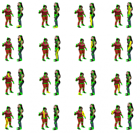
Figure 10. SkeleTrack 23 use for joint proximity measure feature extraction
3.7 Joints stability
Joint stability is the ability of joints to keep their position and function during movement. Many factors affect stability, including muscle strength and joint integrity. In terms of human interaction recognition, joint stability analysis allows quantifying how one can regulate coordinated movement without compromising stability and control. We find that in dynamic interactions where many multiple joints are engaged simultaneously, this feature is critical to the solution speed. We show that via tracking joint movements over time, stability metrics can be derived from tracking joint movements over time in computer vision applications. Systems can use these metrics to discover when two moving objects are stable, like walking together, or unstable, like stumbling or falling.
The stability of a joint refers to the ability of a joint to remain in position effectively in motion. Factors influencing those include muscle strength and joint integrity. A way to quantify joint stability is through the stability index SI, defined in Eq. (10):
$S I=\frac{F_m}{F_l}$ (10)
where, Fm is the force exerted by the muscles surrounding the joint, and Fl is the force applied by the ligaments at the joint.
We assess how well people can move together without losing balance, that is, how stable they are, with stability analysis. For example, in dynamic interactions such as dancing and sports, high stability does imply almost perfect performance and low risk of injury. Stability metrics can be monitored to allow systems to provide feedback on movement efficiency in interactions.
Another unique aspect is that, in combination with feature extraction techniques using skeleton model, relative joint angles can indicate angular relations among joints, proximity measures can express spatial compositions of joints, and stability measures can examine how well the joints stay in place under stresses. When combined, these features add to the capability of human interaction recognition systems without focusing on understanding body mechanics in various contexts. By integrating these techniques into computer vision applications, we achieve more accurate real-time gesture and social interaction interpretation.
Our 23-joint skeleton model extends conventional skeleton models such as OpenPose (18 joints) and Kinect (25 joints) by introducing novel joint definitions focused on fine-grained hand and torso articulation. Table 1 below compares key features:
Table 1. Compares key joint features for the skeleton model
|
Model |
# Joints |
Focus Areas |
Advantages |
Limitations |
|
OpenPose |
18 |
Standard body joints |
Widely used, open source |
Limited hand detail |
|
Kinect v2 |
25 |
Body, hands, feet joints |
Detailed tracking, real-time |
Requires special hardware |
|
Proposed |
23 |
Added hand wrist and heel |
Balances detail and efficiency |
Needs validation in dynamic backgrounds |
The proposed model targets robust HAR in smart home environments, balancing joint detail and computational feasibility, providing improved accuracy for interaction gestures such as handshakes and high-fives.
3.8 Features optimization
Efficient feature selection based on fuzzy optimization attracts attention towards various complex types of datasets. It uses fuzzy logic to quantify the evolution and overlap of feature importance, bringing more complexity to the evaluation than binary methods in traditional approaches. Selection by fuzzy optimization considers multitenancy, notably the importance of features, their potential redundancy with other features between which significant correlation persists, and frequency, to holistically identify the ideal set of features that yields enhanced class separation and elevated predictability. Consequently, it is highly advantageous in tasks that call for machine learning and pattern recognition, as it is pivotal to distinguish the relevant qualities from those that are redundant to construct successful models and make rational decisions. Fuzzy optimization enables the capture of valuable insights from datasets that are characterized by a high number of dimensions. Furthermore, its application improves the performance and interpretability of models, as demonstrated in Figure 11.
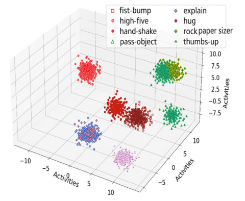
Figure 11. Discrimination of features over the ShakeFive2 dataset
Fuzzy logic differs from traditional binary logic by allowing features partial membership in the set of relevant features. Each feature is assigned a membership grade $\mu(x i) \in[0,1]$ reflecting the degree to which it is relevant for the task. Because of this flexibility, features can be chosen with different levels of importance, unlike the usual approach that only allows features to be either included or excluded.
Fuzzy logic helps to select the best features by considering the following:
3.8.1 Handling of uncertainty and redundancy
Traditional feature selection methods may overlook the subtle interactions between features, especially when features are correlated or partially redundant. Fuzzy logic handles the uncertainty and redundancy by allowing for partial membership.
3.8.2 Feature-class of separability:
The membership grades μ(xi) are computed based on the separability of features with respect to the target activity classes. This ensures that features contributing to distinguishing between classes are given higher importance.
3.8.3 Function of objective
The fuzzy optimization technique optimizes an objective function in which membership degree indicating the relevance of the feature. This optimization process selects a subset of features that balances discriminative power while reducing redundancy.
This fuzzy optimization approach improves the robustness of feature selection by accounting for partially relevant features and reducing the risk of discarding useful features. As a consequence, it improves the accuracy of classification, mainly for complex and large datasets.
$F(X)=\sum_{i=1}^n w_i \cdot \mu\left(x_i\right)$ (11)
In Eq. (11), F(X) is the fuzzy optimization function, which depends on the input set X having (n) elements. Each element xi is associated with a membership value μ(xi), which is the grade to which xi belongs to a particular fuzzy set. The function also uses weights wi to represent the importance or significance that must be given to each element in the optimization process.
Figure 11 depicts the discrimination of features over the ShakeFive2 dataset, it shows how different characteristics or attributes within the dataset are being analyzed and distinguished. By examining the data closely, researchers are able to identify patterns, variations, or unique traits that help them understand and differentiate between these features. This analysis provides valuable insights and knowledge about the dataset, which can be used for further research or decision-making in healthcare monitoring and analysis.
A short description of the datasets employed, the experiments conducted, and their outcomes have been provided.
4.1 Description of dataset
4.1.1 ShakeFive2 dataset
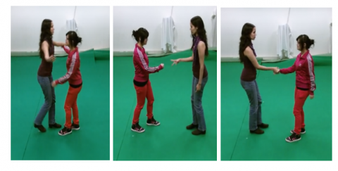
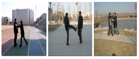
The ShakeFive2 includes 25 participants (15 male, 10 female) aged 20–45 performing eight dyadic activities such as handshake and high-five. Videos were recorded indoors under controlled lighting conditions using a fixed frontal camera at 640×480 resolution and 30 FPS. The dataset contains 150 clips, each approximately 10 seconds in length. ShakeFive2 focuses on dyadic human activities in the dataset, sample shown in Figure 12.
Figure 12. Sequences of the sample frame of ShakeFive2
The dataset comprises 8 different modes of Action: Handshake, Fist bump, Hug, Pass object, High five, Rock-paper-scissors, Thumbs up, and explaining. With this dataset under our examination, our study aims to discover intricate connections and the general patterns among these human communications.
4.1.2 BIT-interaction dataset
The BIT-Interaction consists of 30 participants (18 male, 12 female), aged 18–50, performing eight interaction actions such as boxing and hugging. Videos were recorded in dynamic outdoor environments with varying backgrounds, lighting conditions, and partial occlusions, not in a lab setting with static backgrounds. The videos were captured at 640×480 resolution and 30 FPS, totaling 200 clips, with each clip ranging from 8 to 15 seconds in length. These videos give examples of real people interacting with one another in multiple ways, i.e., shaking hands, hugging, kicking, patting, pushing, giving high-fives, being in a band, and boxing, sample shown in Figure 13. The total dataset is fairly large, consuming approximately 4.4 GB of storage. The video was shot with a very good camera, so that you can clearly see the interrelations between the people. The dataset was processed to find details required by our classification system, which is CNN-based. After that, we employed this modified dataset to evaluate the performance of our new approach.
Figure 13. Sequences of the sample frame of BIT-interaction
4.2 Experimental analysis
All the computing and trials have been carried out on a laptop with Intel Core i7-9th generation, 9850H CPU @2.60 GHz and a 64–bit Windows 11.
4.2.1 Convolutional neural network
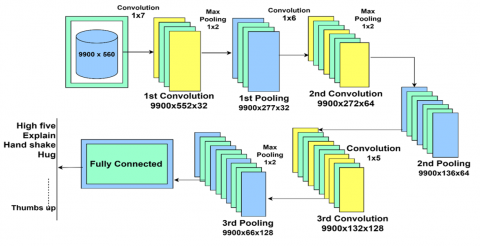
We need human interaction recognition as a typical and more important task. Input data can figure out and classify different activities with CNN. Then, CNNs can look at features that are already extracted. Such data captures spatial and temporal patterns that provide chances to identify activities such as hug, punch, push, or other specified activities. CNNs can learn to recognize human activities with high accuracy and can be deployed in real time systems, e.g., fitness trackers and health care and sports analytics monitoring systems. Figure 14 shows the architecture of human interaction recognition.
We need human interaction recognition as a typical and more important task. Input data can figure out and classify different activities with CNN. Then, CNNs can look at features that are already extracted. Such data capture such spatial and temporal patterns that provide chances to identify activities such as hug, punch, push or other specified activities. CNNs can learn to recognize human activities with high accuracy and can be deployed in real time systems, e.g., fitness trackers and health care and sports analytics monitoring systems. Figure 14 shows the architecture of human interaction recognition.
Figure 14. System architecture illustration of 1-D CNN
4.2.2 Convolutional layers
The CNN architecture is made up of three convolutional layers. CNNs are based on convolutional layers which control the perception of spatial hierarchies of features from input data. For HIR, the pre extracted features are fed directly to Convolutional layers for classification. The first convolutional layer uses 1×7 sized 32 filters, resulting in an output feature map of size 9900×552×32. This dimension is calculated with valid padding. The second convolutional layer has 64 filters of size 1x6 and outputs 9900x272x64. The third convolutional layer has 128 filters of size 1x5, so we have 9900×132×128 as output. We also want to mention that after each convolutional layer, we add activation functions ReLU and bias terms to improve model performance.
$C w^{\{(m+1)\}}(x, y)=\operatorname{ReLU}(i)$ (12)
In Eq. (12), is the activation value of a neuron located at the position (x, y) of a feature map in a convolutional layer after convolutional layer in the CNN. We first need to compute i, which is a weighted sum of the previous layer’s inputs plus a bias term, and then we just multiply that with a frame drop probability to get this value. This process is made possible by the ReLU activation function, which brings much needed nonlinearity to the network. ReLU is essentially only looking at the input i it puts at 0 if u is smaller than zero and at u if u is positive, thus it only looks at values greater than zero.
$\begin{gathered}\operatorname{ReLU}(i)=\sum_{\{a=1\}}^{\{w\}} \Omega[x, d,(y-1)+ \left.\frac{z+1}{2}\right] W^{\{y\}[x, d]}+k_{\{d\}}^{\{z\}}\end{gathered}$ (13)
In Eq. (13), it computes in detail how the ReLU| activation for a specific neuron in CNN is computed. This is a sum over some range of values that are probably different values of the previous channel (or feature) from which these vectors are derived. The notation $\Omega\left[x, d,(y-1)+\frac{z+1}{2}\right]$ denotes accessing data from a multi-dimensional array or tensor, i.e. the inputs or the feature maps. The weight for each feature or channel is given by $W^{\{y\}[x, d]}$ and the bias term $k_{\{d\}}^{\{z\}}$ multiplies all output. The network processed different inputs and applied its learned parameters to generate meaningful activation values, so the network learns complicated patterns and makes predictions.
4.2.3 Pooling layers
Down sampling of feature maps and generating information summaries are the main uses of pooling layers. It simplifies the following layers and saves computation. For each convolution layer, we down sample the feature maps with max pooling layer and reduce their size. Window is 1×2, draining 1/2 on a spatial reduction of the feature vector axis get 9900×277×32. Similar on to the second and third pooling layers use 1×2 max-pooling to give outputs of the size of 9900×136×64 and 9900×66×128.
$P L^{\{q\}}(x, y)=\max \left(C v^{\{q\}(x,((y-1) t(a+b)))}\right)$ (14)
In Eq. (14), $C_v$ is the feature map pooling the feature map at position (i,j) in the context of a neural network. The area of input feature map being examined by pooling window and specific to that window is denoted by convolutional layers. This area selects the maximum value in this pooling operation, down sampling the feature map and shrinking its size.
4.2.4 Fully connected layers
The classification component of the CNN is the most important part of the Fully Connected Layers. The previously extracted features' inputs meet these layers and make decisions on learned representations. As a result, the CNN can capture intricate relationships among the features and the interaction classes. Then, the fully connected layers carry out matrix multiplications and nonlinear transformations to transform these pre extracted features to class probabilities or scores to exactly classify and recognise or recognize the human activities images.
The Adam optimizer was used to train CNN, batch size 64, initial learning rate 0.001 and cross-entropy loss function. The training was to last 50 epochs. To avoid overfitting, a dropout rate of 0.5 was used after fully connected layers. Data augmentation such as random horizontal flips and small rotations as used to enhance robustness. The training was done on NVIDIA RTX 3060 GPU with 12GB RAM.
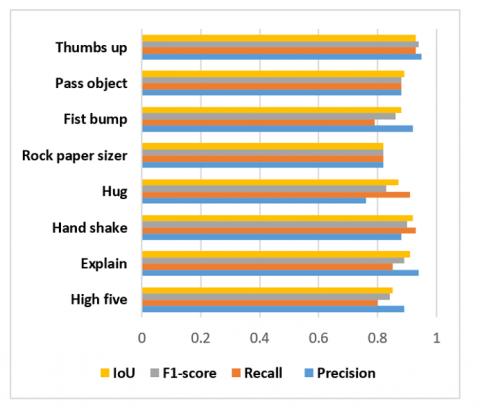
In our research work, we have used embedded CNN as a classifier to test our novel approach. An experiment was conducted with great care and a lot of attention to detail and the data were thoroughly analyzed. In order to evaluate the performance of the classifier in a detailed manner, several metrics including accuracy, recall, and F1-score measures were used to obtain the overall accuracy of the classifier. The effectiveness evaluation of the classifier demonstrated that the CNN-based method is rather successful with the accuracy of 88%. This fact demonstrates that the suggested approach can be used in the practical applications. The results of the ShakeFive2 dataset classification are presented in Table 2 below and contain precision, recall, and F1-score, and are compared in Figure 15.
Table 2. Performance of recall, precision, and F1 score over ShakeFive2
|
Action Activities |
Precision |
F1-Score |
Recall |
|
High five |
0.89 |
0.84 |
0.80 |
|
Explain |
0.94 |
0.89 |
0.85 |
|
Hand shake |
0.88 |
0.90 |
0.93 |
|
Hug |
0.76 |
0.83 |
0.91 |
|
Rock paper sizer |
0.82 |
0.82 |
0.82 |
|
Fist bump |
0.92 |
0.86 |
0.79 |
|
Pass object |
0.88 |
0.88 |
0.88 |
|
Thumbs up |
0.95 |
0.94 |
0.93 |
|
Weighted Average |
0.89 |
0.88 |
0.88 |
|
Macro Average |
0.88 |
0.87 |
0.86 |
Figure 15 shows performance assessment of a classification model on ShakeFive2 dataset.
Figure 15. Precision, recall, and F1 score for each class on ShakeFive2 dataset
Table 3 provides the Intersection over Union (IoU) score for various classes of the ShakeFive2 Interaction dataset IoU is used very often to assess the qualities of the object detection models. A higher IoU means better localization accuracy thus the proposed method of using IoU has been proven to have better results.
Table 3. Intersection over Union over ShakeFive2 Interaction dataset
|
Action Activities |
IoU |
|
High five |
0.85 |
|
Explain |
0.91 |
|
Hand shake |
0.92 |
|
Hug |
0.87 |
|
Rock paper sizer |
0.82 |
|
Fist bump |
0.88 |
|
Pass object |
0.89 |
|
Thumbs up |
0.93 |
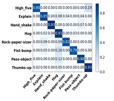
Figure 16 shows that the confusion matrix offers the following quick breakdown in the classification analysis of a model on the ShakeFive2 and BIT-interaction datasets. It gives the total number of samples identified for each class, both the total number of samples identified consistently and the total number of samples misidentified. Figure 17 and Table 4 show training loss and accuracy curve over 50 epochs for the ShakeFive2 dataset.
Figure 18 shows training loss and accuracy curve over 50 epochs for the ShakeFive2 dataset.
Figure 16. Confusion matrix for ShakeFive2
Figure 17. Training loss curve over 50 epochs for the ShakeFive2 dataset, illustrating steady decrease in loss, indicating model convergence
Table 4. Results for accuracy and loss ShakeFive2 dataset
|
Epoch |
Loss |
Accuracy |
|
1 |
1.2248 |
0.5065 |
|
2 |
1.1747 |
0.5001 |
|
4 |
1.2210 |
0.5355 |
|
8 |
0.9523 |
0.6106 |
|
16 |
0.6264 |
0.7767 |
|
32 |
0.4021 |
0.8750 |
|
40 |
0.3571 |
0.8869 |
|
45 |
0.3368 |
0.8906 |
|
50 |
0.3017 |
0.8834 |
Figure 18. Training accuracy progression over 50 epochs for the ShakeFive2 dataset
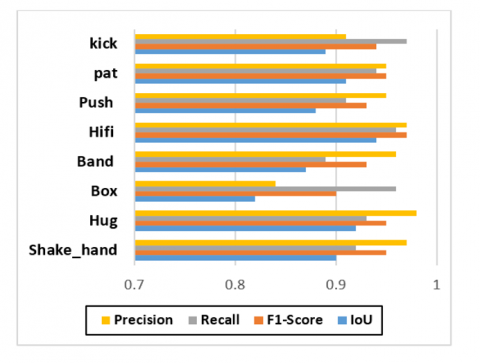
Figure 19. Precision, recall, and F1 score for each class on BIT interaction dataset
The results of the ShakeFive2 dataset classification are presented in Table 2 and contain precision, recall, and F1-score, and are compared in Figure 19. Table 5 shows the results over the BIT -Interaction dataset. Table 6 offers the IoU of the different classes of the BIT -Interaction dataset. IoU is employed rather frequently to evaluate the characteristics of object detection models.
Table 5. Recall, precision, and F1-score over BIT -Interaction dataset
|
Action Activities |
Precision |
Recall |
F1-Score |
|
Shake_hand |
0.97 |
0.92 |
0.95 |
|
Hug |
0.98 |
0.93 |
0.95 |
|
Box |
0.84 |
0.96 |
0.90 |
|
Band |
0.96 |
0.89 |
0.93 |
|
Hifi |
0.97 |
0.96 |
0.97 |
|
Push |
0.95 |
0.91 |
0.93 |
|
pat |
0.95 |
0.94 |
0.95 |
|
kick |
0.91 |
0.97 |
0.94 |
|
Weighted Average |
0.946 |
0.945 |
0.945 |
|
Macro Average |
0.947 |
0.941 |
0.943 |
Table 6. Intersection over union over ShakeFive2 Interaction dataset
|
Action Activities |
IoU |
|
Shake_hand |
0.90 |
|
Hug |
0.92 |
|
Box |
0.82 |
|
Band |
0.87 |
|
Hifi |
0.94 |
|
Push |
0.88 |
|
pat |
0.91 |
|
kick |
0.89 |
|
Mean IoU |
0.89 |
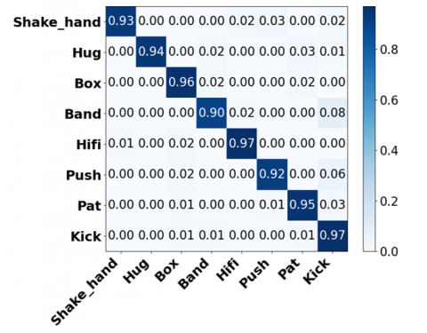
Figure 20 shows that the confusion matrix offers the following quick breakdown in the classification analysis of a model on the BIT-interaction datasets. Figures 21 and 22, and Table 7 show the training loss and accuracy curve over 50 epochs for the ShakeFive2 dataset.
Figure 20. Confusion matrix for BIT-Interaction dataset
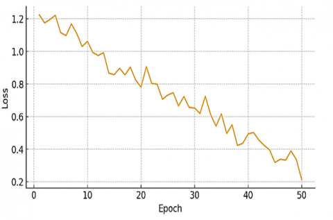
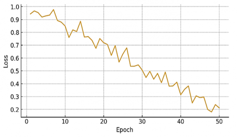
Figure 21. Training loss curve over 50 epochs for the BIT-Interaction dataset, with loss reducing smoothly toward 0.2, indicating effective learning
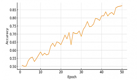
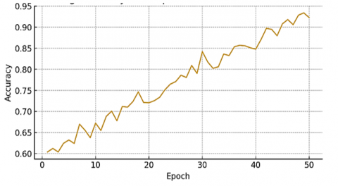
Figure 22. Training accuracy progression over 50 epochs for the BIT-Interaction dataset, demonstrating an increase from about 60% to approximately 94%
Table 7. Results for accuracy and loss BIT-Interaction dataset
|
Epoch |
Loss |
Accuracy |
|
1 |
0.9434 |
0.6038 |
|
2 |
0.9668 |
0.6121 |
|
4 |
0.9189 |
0.6243 |
|
8 |
0.8210 |
0.6866 |
|
16 |
0.6294 |
0.7858 |
|
32 |
0.4365 |
0.8707 |
|
40 |
0.3883 |
0.8875 |
|
45 |
0.3678 |
0.8925 |
|
50 |
0.2017 |
0.9388 |
Table 8. Comparative analysis with other state-of-the-art techniques over both datasets
|
Methods |
BIT-Interaction Accuracy (%) |
ShakeFive2 Accuracy (%) |
|
CNN [23] |
84.63 |
- |
|
White stag Model [24] |
87.50 |
- |
|
Two-stream [25] |
90.63 |
- |
|
Co-LSTM [26] |
92.88 |
- |
|
Deformable parts models [27] |
- |
65% to 87% |
|
HOGHOFMBH [28] |
- |
82% |
|
Proposed Recognition System |
94% |
88% |
Table 8 showns the comparative analysis with other state-of-the-art techniques over both datasets.
Table 9 compares different components' performance (accuracy) in the proposed 23-joint skeleton model. During runtime analysis, the system’s performance was tested using an Intel i7 CPU and NVIDIA RTX 3060 GPU. The system completed inference in about 20 milliseconds per frame, making it possible to run at 30 frames per second, which is ideal for real-time usage in changing environments. The total time it takes to process a 10-second video (300 frames) is about 6 seconds. The lightweight 1-D CNN architecture and optimized feature extraction pipeline reduce computational overhead, making deployment feasible on edge devices common in smart homes. Future optimizations include model pruning and quantization to further improve efficiency.
Table 9. Performance comparison of different components in the proposed model across both datasets: Accuracy and computational feasibility
|
Experiments |
Pre processing |
Silhouette Extraction |
Feature Extraction |
Fuzzy Optimization |
CNN |
23-Joint Skeleton |
ShakeFive2 Accuracy (%) |
BIT-Interaction Acc (%) |
Inference Time (ms/frame) |
FPS |
Computation Time (10s video) |
|
Full Model |
✓ |
✓ |
✓ |
✓ |
✓ |
✓ |
94.0 |
88.25 |
20 ms |
30 FPS |
6 seconds |
|
Without Preprocessing |
✕ |
✓ |
✓ |
✓ |
✓ |
✓ |
87.4 |
85.7 |
25 ms |
28 FPS |
7 seconds |
|
Without Silhouette Extraction |
✓ |
✕ |
✓ |
✓ |
✓ |
✓ |
85.9 |
82.5 |
22 ms |
29 FPS |
6.5 seconds |
|
Without Feature Extraction |
✓ |
✓ |
✕ |
✓ |
✓ |
✓ |
88.2 |
84.8 |
23 ms |
28 FPS |
6.8 seconds |
|
Without Fuzzy Optimization |
✓ |
✓ |
✓ |
✕ |
✓ |
✓ |
89.1 |
85.3 |
22 ms |
29 FPS |
6.2 seconds |
|
Without Preprocessing + Feature Extraction |
✕ |
✓ |
✕ |
✓ |
✓ |
✓ |
82.6 |
77.5 |
28 ms |
26 FPS |
7.5 seconds |
|
Without Preprocessing + Silhouette Extraction |
✕ |
✕ |
✓ |
✓ |
✓ |
✓ |
84.5 |
75.9 |
27 ms |
27 FPS |
7 seconds |
|
With Kinect - 25 Joints) |
✓ |
✓ |
✓ |
✓ |
✓ |
✕ |
88.2 |
94.1 |
21 ms |
30 FPS |
6 seconds |
|
18-Joint Model - OpenPose) |
✓ |
✓ |
✓ |
✓ |
✓ |
✕ |
80.5 |
85.2 |
30 ms |
25 FPS |
8 seconds |
Table 10. Statistical validation of model performance
|
Dataset |
Accuracy (%) |
Std. Dev. |
p-value vs. Baseline |
|
ShakeFive2 |
88.2 |
1.5 |
0.007 |
|
BIT-Interaction |
94.1 |
1.2 |
0.004 |
To assess statistical significance, we performed 5-fold cross-validation, reporting mean accuracy ± standard deviation. The proposed system achieved 88.2% ± 1.5% on ShakeFive2 and 94.1% ± 1.2% on BIT-Interaction. Paired t-tests against baseline CNN models showed p-values < 0.01, indicating statistically significant improvements.
Table 10 shows the mean accuracy, std, and p-values from paired t-tests comparing the proposed model to baseline CNN models.
Our research introduces a robust framework for recognizing human interactions, integrating advanced techniques across multiple stages. Using a five-step methodology, we’ve significantly improved the accuracy and efficiency of identifying complex human interactions. First, gamma correction in the preprocessing stage enhanced image quality, providing a solid foundation. The silhouette extraction process, using Multi-Object Tracking and graph-based segmentation, precisely isolated human figures, crucial in crowded or dynamic settings. We combined the BRIEF descriptor with our novel 23 key joint point features for feature extraction, capturing essential spatial and temporal dynamics. Fuzzy optimization techniques added robustness, improving decision-making under uncertainty. Finally, applying CNN for classification, we achieved an impressive 88% accuracy. This multi-faceted approach not only advances human interaction recognition but also overlays the technique for future developments in computer vision.
In future, emphasis will be laid on the privacy concerns and enhancement of the SkeleTrack23 model. Another equally noteworthy drawback that can be mentioned is that removing the background from the videos filmed with immobile cameras is proposed in the system. However, this study might not work if the background settings change from time to time within the data. Therefore, the system will be deployed to more general environmental conditions and data. Future work will be to handle dynamic backgrounds by incorporating adaptive background subtraction methods that are robust to lighting variations and camera motion. Temporal smoothing and attention mechanisms will be added to the SkeleTrack23 model to enhance robustness to occlusions and partial visibility. We are focusing on solving the issue of dynamic backgrounds, which is essential for correcting the recognition of human activities in real environments. For this reason, we recommend using background subtraction and motion-based segmentation to separate the moving subjects from the busy environment. We also aim to use multi-modal sensor fusion by combining RGB video with depth sensors or IMUs, which should make the system more reliable when changing light and when objects are hidden.
Real-time performance is another area we want to concentrate on. Even though the method performs well in real time, more improvements, such as model pruning and quantization, are needed to make it work well on edge devices with limited resources.
Princess Nourah bint Abdulrahman University, Riyadh, Saudi Arabia. Princess Nourah bint Abdulrahman University Researchers Supporting Project number (PNURSP2025R440), Princess Nourah bint Abdulrahman University, Riyadh, Saudi Arabia.
[1] Kamthe, U.M., Patil, C.G. (2018). Suspicious activity recognition in video surveillance system. In Proceedings of the 2018 Fourth International Conference on Computing Communication Control and Automation (ICCUBEA), Pune, India, pp. 1-6. https://doi.org/10.1109/ICCUBEA.2018.8697408
[2] Saleem, G., Bajwa, U.I., Raza, R.H. (2023). Toward human activity recognition: A survey. Neural Computing and Applications, 35(5): 4145-4182. https://doi.org/10.1007/s00521-022-07937-4
[3] Li, Y., Yang, G., Su, Z., Li, S., Wang, Y. (2023). Human activity recognition based on multi environment sensor data. Information Fusion, 91: 47-63. https://doi.org/10.1016/j.inffus.2023.03.002
[4] Abdel-Aty, M., Wu, Y., Zheng, O., Yuan, J. (2022). Using closed-circuit television cameras to analyze traffic safety at intersections based on vehicle key points detection. Accident Analysis and Prevention, 176: 106794. https://doi.org/10.1016/j.aap.2022.106794
[5] Shdefat, A.Y., Mostafa, N., Al-Arnaout, Z., Kotb, Y., Alabed, S. (2024). Optimizing HAR systems: Comparative analysis of enhanced SVM and k-NN classifiers. International Journal of Computational Intelligence Systems, 17(1): 150. https://doi.org/10.1007/s44196-024-00554-0
[6] García, S.M., Baena, C.H., Salcedo, A.C. (2023). Human activities recognition using semi-supervised SVM and hidden Markov models. TecnoLógicas, 26(56): e2474. https://doi.org/10.22430/01237799202356e2474
[7] Rao, D.S., Rao, L.K., Bhagyaraju, V., Meng, G.K. (2024). Enhanced depth motion maps for improved human action recognition from depth action sequences. Traitement du Signal, 41(3): 1461-1472. https://doi.org/10.18280/ts.410334
[8] Gao, X. (2024). Explore the ancient roots of the Huaxia people and Chinese civilization. International Journal of Anthropology and Ethnology, 8(1): 10. https://doi.org/10.1186/s41257-024-00111-9
[9] Zahoor, L., Jalal, A. (2024). Drone-based human surveillance using YOLOv5 and multi-features. In 2024 International Conference on Frontiers of Information Technology (FIT), Islamabad, Pakistan, pp. 1-6. https://doi.org/10.1109/FIT63703.2024.10838465
[10] Rahevar, M., Ganatra, A., Saba, T., Rehman, A., Bahaj, S.A. (2023). Spatial–temporal dynamic graph attention network for skeleton-based action recognition. IEEE Access, 11: 21546-21553. https://doi.org/10.1109/ACCESS.2023.3247820
[11] Hossen, M.A., Abas, P.G.E. (2025). Machine learning for human activity recognition: State-of-the-art techniques and emerging trends. Journal of Imaging, 11(3): 91. https://doi.org/10.3390/jimaging11030091
[12] Tayyab, M., Jalal, A. (2025). Disabled rehabilitation monitoring and patients healthcare recognition using machine learning. In 2025 6th International Conference on Advancements in Computational Sciences (ICACS), Lahore, Pakistan, pp. 1-7. https://doi.org/10.1109/ICACS64902.2025.10937871
[13] Khameneh, Z., Ghaznavi, M., Kilicman, A., Mahad, Z., Mardani, A. (2024). A maximal-clique-based clustering approach for multi-observer multi-view data by using k-nearest neighbor with S-pseudo-ultrametric induced by a fuzzy similarity. Neural Computing and Applications, 36(16): 9525-9550. https://doi.org/10.1007/s00521-024-09560-x
[14] Khan, U., Pao, W., Pilario, K.E.S., Sallih, N., Khan, M.R. (2023). Two-phase flow regime identification using multi-method feature extraction and explainable kernel Fisher discriminant analysis. International Journal of Numerical Methods for Heat & Fluid Flow, 34(8): 2836-2864. https://doi.org/10.1108/HFF-09-2023-0526
[15] Mekruksavanich, S., Jantawong, P., Jitpattanakul, A. (2022). LSTM-XGB: A new deep learning model for human activity recognition based on LSTM and XGBoost. In Proceedings of the 2022 Joint International Conference on Digital Arts, Media and Technology with ECTI Northern Section Conference on Electrical, Electronics, Computer and Telecommunications Engineering (ECTI DAMT & NCON), Chiang Rai, Thailand, pp. 342-345. https://doi.org/10.1109/ECTIDAMTNCON53731.2022.9720409
[16] Nematallah, H., Rajan, S. (2024). Adaptive hierarchical classification for human activity recognition using inertial measurement unit (IMU) time-series data. IEEE Access, 12: 52127–52149. https://doi.org/10.1109/ACCESS.2024.3386351
[17] Qi, M., Cui, S., Chang, X., Yin, T. (2022). Multi-region nonuniform brightness correction algorithm based on L-channel gamma transform. Security and Communication Networks, 2022: 2675950. https://doi.org/10.1155/2022/2675950
[18] Luo, W., Xing, J., Milan, A., Zhang, X., Liu, W., Kim, T.K. (2021). Multiple object tracking: A literature review. Artificial Intelligence, 293: 103448. https://doi.org/10.1016/j.artint.2020.103448
[19] Zheng, L., Tang, M., Chen, Y., Zhu, G., Wang, J., Lu, H. (2021). Improving multiple object tracking with single object tracking. In Proceedings of the IEEE/CVF Conference on Computer Vision and Pattern Recognition (CVPR), Nashville, USA, pp. 2453-2462. https://doi.org/10.1109/CVPR46437.2021.00246
[20] Yang, H.Z., Wang, Y.T., Yang, J., Liu, Y. (2010). A novel graph cuts based liver segmentation method. In Proceedings of the 2010 International Conference on Medical Image Analysis and Clinical Application (MIACA), Guangzhou, China, pp. 50-53. https://doi.org/10.1109/MIACA.2010.5528409
[21] Qin, Y., Mo, L., Li, C., Luo, J. (2020). Skeleton-based action recognition by part-aware graph convolutional networks. The Visual Computer, 36: 621-631. https://doi.org/10.1007/s00371-019-01644-3
[22] Luvizon, D.C., Tabia, H., Picard, D. (2017). Learning features combination for human action recognition from skeleton sequences. Pattern Recognition Letters, 99: 13-20. https://doi.org/10.1016/j.patrec.2017.02.001
[23] Jalal, A., Mahmood, M., Hasan, A.S. (2019). Multi-features descriptors for human activity tracking and recognition in indoor-outdoor environments. In Proceedings of the 16th International Bhurban Conference on Applied Sciences and Technology (IBCAST), Islamabad, Pakistan, pp. 371-376. https://doi.org/10.1109/IBCAST.2019.8667145
[24] Kong, Y., Jia, Y., Fu, Y. (2012). Learning human interaction by interactive phrases. In Computer Vision-ECCV 2012: 12th European Conference on Computer Vision, Florence, Italy, pp. 300-313. https://doi.org/10.1007/978-3-642-33718-5_22
[25] Donahue, J., Hendricks, L.A., Rohrbach, M., Venugopalan, S., Guadarrama, S., Saenko, K., Darrell, T. (2015). Long-term recurrent convolutional networks for visual recognition and description. In Proceedings of the IEEE Conference on Computer Vision and Pattern Recognition (CVPR), Boston, USA, pp. 2625-2634. https://doi.org/10.1109/CVPR.2015.7298878
[26] Shu, X.B., Tang, J.H., Qi, G.J., Song, Y., Li, Z.C., Zhang, L.Y. (2017). Concurrence-aware long short-term sub-memories for person-person action recognition. In Proceedings of the IEEE Conference on Computer Vision and Pattern Recognition Workshops (CVPRW), pp. 1-8.
[27] van Gemeren, C., Poppe, R., Veltkamp, R.C. (2018). Hands-on: Deformable pose and motion models for spatiotemporal localization of fine-grained dyadic interactions. EURASIP Journal on Image and Video Processing, 2018(1): 16. https://doi.org/10.1186/s13640-018-0255-0
[28] Van Gemeren, C., Tan, R.T., Poppe, R., Veltkamp, R.C. (2014). Dyadic interaction detection from pose and flow. In Proceedings of the International Workshop on Human Behavior Understanding, pp. 101-115. https://doi.org/10.1007/978-3-319-11839-0_9