Sourabh Pandey*![]() | Prashant Kumar Jain
| Prashant Kumar Jain![]() | Prabhat Patel
| Prabhat Patel![]()
© 2025 The authors. This article is published by IIETA and is licensed under the CC BY 4.0 license (http://creativecommons.org/licenses/by/4.0/).
OPEN ACCESS
In low-cost portable cameras and camcorders, simple and fixed lens configurations are used. Items outside of the depth range appear fuzzy due to the short depth of focus of these cameras. Furthermore, videos taken with a hand-held camera include severe handshakes with jitters. As a result, it is critical to stabilize camera motions to increase video quality. Previous video stabilization (VS) solutions included de-blurring at the post-processing stage, resulting in erroneous measurement of motion parameters. To eliminate these estimation errors, this research suggests including de-blurring before implementing motion estimation (ME). The brightness of each pixel is convolved with the square of orthogonal temporal derivatives as a newly modified proposed blurriness index, which represents magnified objects and background motions. The proposed VS method to smooth the accidental motions and jitters in the movie has utilized an adaptive FIR filter. The simplified edge completion approach is designed to produce full-frame stabilized video sequences. The suggested method may accurately identify blurry frames at a cheap computational cost. Results present the performance comparison of the proposed blurriness index with the two most commonly used blurriness indexes. De-blurring the video before motion estimation improves the video stabilization quality.
blurriness index, computer vision video stabilization, motion smoothing, motion compensation, edge completion video de-blurring
Video stabilization (VS) systems have undergone substantial evolution to solve problems, such as camera jitter and visual distortion [1]. To improve the stabilization quality, the VS process employs several techniques, including motion decomposition and smoothing. Videos captured with handheld cameras frequently suffer from undesired camera motion and blur during the scene capture period. The precision of motion estimate largely determines how well Video Stabilization (VS) works. Motion has been estimated using techniques based on features [2-4] and global estimation approaches [5, 6] feature-based approaches are limited to local effects, and their efficacy varies depending on the method used to select the feature points. Direct pixel-based approach [7] is both fast and computationally demanding. As a result, it is necessary to lower the computational cost of these algorithms.
Another typical issue is the compounding blurring effect observed in videos [7]. All forms of blur, including motion, depth-of-field (DOF), and sharpness, may not be sufficiently represented by the existing blurriness index (BI). The major problem of research is the selection of a suitable BI for the efficient detection of blurry frames in a video. Furthermore, selecting an incorrect BI can make the stabilization process overly susceptible to video noise. In the study by Rawat and Singhai [7], de-blurring methods are employed as preprocessing stages to remove blur from video frames. However, the major issue is that the computational cost of de-blurring may be high, particularly in applications that operate in real time. Furthermore, research has been conducted on the application of temporal derivatives for motion estimation to enhance the stabilization performance, particularly when large moving objects are present [8]. By lowering blurriness and raising overall video quality, de-blurring approaches with temporal derivatives as well as motion smoothing, can be combined to further improve VS quality. The goal of these developments is to offer viewers a better visual experience by providing more reliable and effective VS options for a variety of difficult movies. To solve these problems, this study proposes the use of a modified blurriness index capable of repressing the much better edges of motion components, and thus, it is better to identify even a small number of blurry frames. The modified BI is capable of repressing blurring due to object motion. A "washed-out" appearance and the loss of tiny details are possible consequences of aggressive motion smoothing. It can be difficult to strike an ideal mix between detailed preservation and stability. Therefore, the FIR filter is proposed in this paper for motion smoothing, which has relatively less delay and is capable of stabilizing the motion while keeping the missing areas on the lower side.
Blur is present as a result of the attenuation of high spatial frequencies in video frames, which only takes place in specific circumstances, such as severe handshakes or jitter, massive and quick object movements, optical zooming, extended exposure times, or non-uniform lighting or illumination. Furthermore, most smartphone cameras have a shallow DoF [9]. Consequently, individuals can only focus on items within a certain depth span, and objects beyond that range appear hazy. Blur can be spaced differently and may be affected by DoF or object motion. It has various effects on foreground and background objects. The level of blur also fluctuates with the objects or the forward and reverse motions of the camera. As a result, the blur does not affect all frames equally, and blurry frames must be identified before the video sequence is de-blurred. Known algorithms have not examined the influence of blur upon motion estimation, hence most known techniques include de-blurring following motion estimation. In a video taken with a handheld camera or camcorder, the foreground items are frequently independently moving objects towards the camera, whose movements differ from those of the complete background or scene. Objects in the backdrop, on the other hand, are normally static in the scene, and distortion can be seen at their margins owing to camera tremors and motions. Background items are often further away from the camera and thus are blurrier. Because of the small size of hand-held cameras, the aperture with lens assembly is small. Camera tremors affect a variety of camera characteristics, causing the scene to become blurry. Employing efficient VS can frequently allow for 2-4 folds lower shutter speeds (compared with 4-16 folds longer exposure times), while considerably slower effective speeds can be attained. Thus, video stabilization can overcome the hand-held mobile camera's slow shutter speed constraint. As a consequence, de-blurring the video clip before might improve VS performance.
1.1 Contributions of work
This research proposes the design of an efficient VS method that works equally well for fast and slow-moving objects. The major contributions of this study are as follows:
Initially, it was proposed to deblur the video sequence before being stabilized. To justify this statement a mathematical model was provided to highlight the impact of blur for motion estimation. The performances of three blurring methods were compared for the VS. A modified blurriness index is proposed using temporal derivatives and is then used for the motion estimation process. The effectiveness of VS is evaluated via quantitative analysis for the six different kinds of motions using existing and proposed blurriness index profiles. Various filter performances are evaluated along with the proposed FIR filter along with the motion compensation. The proposed work employed the FIR filter with optimum filter coefficient selection, which nearly eliminated the requirement of Gaussian kernel-based MC algorithm and efficiently stabilized the video. A fast and simple edge completion method is proposed for full-frame stabilized video sequence generation.
In rest of the script review of related works is explained in Section 2. Section 3 explains the effect of moving object and blur on the blurriness index for VS, and Section 4 describes process of motion estimation and smoothing respectively. Section 5 presents the sequential results of proposed VS method. The input video details are presented in section 5.1. Section 5.1 followed by the performance comparison of comparison of VS with proposed and existing blurriness index in section 5.2. Section 5.3 discusses using hierarchical differential global estimation of motion parameters. Section 5.4 describes the motion smoothing using proposed adaptive FIR filters to smooth accumulated global motion parameters. Motion compensation and edge completion methods to generate stabilized videos are explained in sections 5.4.1 and 5.4.2 respectively. Sections 5.5 and 5.6 present the two specific case studies for the large object motion and frame resize attack respectively. Performance at each stage is justified using statistical and objective evaluation of the results. Work is concluded in Section 6 with scopes of future work.
Numerous strategies have been put forth by researchers to effectively stabilize video sequences. To produce stabilized videos, VS approaches are needed and are broadly classified in Figure 1 as global motion estimation, motion smoothing, and motion compensation algorithms. Either directly pixel-based methods or feature-based methods can be used to estimate global motion.
Figure 1. Broad classification diagram of the VS methods
2.1 Review of feature based VS methods
There are many feature based VS methods available in the literature. Wang et al. [1] proposed to solve problems like camera jitter and visual distortion; video stabilization (VS) systems have undergone substantial evolution of motion decomposition method. Many researchers [2, 3] have employed SIFT features to eliminate the p additionally, an adjusted Chauvenet parameter is used in the method to identify and suppress outlier features, purposeful inter-frame motions by lining up the feature points. Luchetti et al. [4] devised a way for making 360 videos viewing more fluid and enjoyable for watching. To begin, the motions are produced employing an innovative approach that employs a Particle Swarm Optimization approach while accounting for the estimation of uncertainty among features. A modified Chauvenet parameter is also utilized to locate and suppress outlier features in the algorithm. The method appears to be a little hazy for different types of motion.
Lee et al. [5] stabilization process of the video signal plays a significant part in improving the clarity of the image. Early methods for recovering 2D or 3D frame motion in movies faced challenges owing to their reliance on feature tracking, which struggled with local feature mining and tracking in noisy environments. To address this stability issue, recent learning-based approaches have employed deep neural networks to identify frame transformations by using high-level information. In their work, Xu et al. [6] employed Features from Accelerated Segment Test (FAST) method to detect features in individual frames. Subsequently, a rapid binary descriptor based on Binary Robust Independent Elementary Features (BRIEF) was used to match the corresponding features between consecutive frames. The combination of aligned FAST and rotated BRIEF, known as ORB, is particularly effective for feature detection and matching and accelerating motion prediction without the need for hardware enhancement. Furthermore, an improved motion smoothing technique that utilizes linear models to smooth motion variables without requiring continuous global motion estimation is proposed. The speed of the feature-based approaches depends greatly on how well the feature point selection is done. There may be few good features in scenes that have inadequate texture, repetitive patterns, or severe blur, which might result in erratic tracking and subpar stabilization. Additionally, feature based methods may not be able to reliably capture complicated camera actions like zooming and rolling shutter distortion, which could result in errors affecting the stabilized footage. For predicting slow inter-frame motion, such as in handheld videos, direct pixel-based approaches are used.
2.2 Review of global direct video stabilization methods
Many VS methods use direct pixel based approaches. Rawat and Singhai [7] presented a comparative analysis of VS with different temporal derivatives. These derivatives include two- and four-point central differences and simple pixel difference approaches. It was observed that different derivatives responded differently to different occasions. Farid and Woodward [8] applied a direct pixel-based technique, which minimizes the quadratic error function for estimating motions via Taylor series expansion. Matsushita et al. [9] proposed a direct full-frame VS approach based on multilayer differential motion estimation. This technique employs motion-in-painting to provide a complete video frame. Choi et al. [10] proposed a novel method for real-time video stabilization that transforms shaky video into a video that is maintained as if it were stabilized in real time using gimbals. Our design can be trained without the use of particular equipment (such as two stereo cameras or additional motion sensors), as it can be trained without supervision. Our system comprises a transformation estimator between specified frames for modifications to the overall stability, then a scene motion control module using temporally normalized optical flow for greater stability.
Shi and He [11] evaluated various ME techniques used in VS, including mechanical and optical approaches. Their study focused on challenges in stabilizing video from handheld cameras, which are particularly susceptible to inadvertent movements. Barron et al. [12] have proposed a good 4-point central difference method for ME. The method is adopted in current research for VS applications. Pang et al. [13] have used a dual tree-based wavelet transform application for VS. An extended video feature extraction method is presented in the book by Bovik [14]. But these methods are simple and are suitable for slow object motion. Yu and Ramamoorthi [15] have suggested a unique neural network (NN) approach to derive optical flow fields of the input video from the per-pixel shift fields needed for video stabilization. In contrast to other video stabilization methods that use machine learning to indirectly infer frame movements from color videos, our approach employs an optical flow to directly analyze motion and learn stabilization. They also suggested an optical flow-based pipeline. Yu et al. [16] system relies on gated transformations trained using millions of images. The proposed closed multiplication addresses the limitations of vanilla convolution, which treats all input images as valid, by implementing a learnable dynamic feature-selection process for each channel at every spatial location across all layers. This approach applies partial compression and resolves the issues associated with standard convolution techniques. Additionally, global and local GANs created for a single rectangle mask are not suitable because free-form masks can exist everywhere in images of any shape. e Souza et al. [17] stated that the growth of multimedia data has helped many applications, like telemedicine, business video conferencing, monitoring and protection, entertainment, remote learning, and robotics. The VS is a technique for detecting and identifying removing motion or instabilities from a video channel that is put on by handling the camera during the recording phase. Souza presents and examines a unique approach that uses local features to identify errors in the camera's global motion prediction
2.3 Review of motion smoothing
Over 2 decades ago, several methods have been suggested to smooth undesirable camera motions. The VS algorithm utilizing feature point filtering and differential optical flow, was proposed by Cai and Walker [18] in 2009. Unwanted motions were eliminated using a first-order IIR filter. Rawat and Singhai [19] presented a good use of the IIR filter for motion smoothing of a video sequence for VS. They also considered the Taylor series expansion method for the ME and global motion-smoothing approaches. Muthu et al. [20] researched stationary, small, or slow-moving objects that, when covered, can improve the results of motion classification but are frequently missed by standard methods. Our method integrates motion inputs with logical object-based segmentation to identify the total moving objects and their motion characteristics and to execute segmentation. To calculate the object-specific motion parameters, connection matching and selected object-based samples were used. Wang et al. [21] leading to substantial improvements in video stabilization. On the other hand, previous surveys have primarily focused on traditional methodologies and lack comparative performance. Wang et al. [21] have provided an outstanding assessment of VS techniques for various types of motions and applications. Kumar et al. [22] proposed quadratic smoothing for VS problem resolution. Wang and Huang [23] recently developed a global pixel-based VS technique using motion smoothing.
Liu et al. [24] present an article that offers a frame generation technique for stabilizing full-frame video. They first calculated the strong warping fields from nearby frames and then merged the warped elements to create a stable image. Our main technical innovation is the learning-based hybrid space combination, which reduces errors produced by incorrect optical flow and fast-moving objects. Rawat and Sawale [25] have published the application of Gaussian kernel filtering (GKF) for VS tasks. The GKF method is widely used for motion compensation (MC) in full-frame VS applications. However, excessive kernels may lead to over-blurriness in a video sequence. Thus, this study focuses on designing a smoothing approach that eliminates the requirement of the GKF. This method is specific to trajectory-based approaches. Zhao and Ling [26] presented a pixel-based warping approach for video stabilization. However, it is necessary to design simple algorithms and reduce the computational cost of this stage for the MC. Mosleh et al. [27] used good use of a simple edge completion method for efficient VS and MC. They also used an IIR filter with a GKF for smoothing motions. Shankarpure and Abin [28] considered the frame–to–frame approach for VS by removing the Jitter method to be slow. To discover the temporal derivatives, a method using 1D separable kernel filters was applied.
A fast VS technique based on block matching and edge completion was proposed by Tang et al. [29] in 2011. Souza and Pedrini [30] have designed a camera trajectory filtering method for the VS task. Yang et al. [31] have demonstrated a good use of the particle filter but for the specific case of the profile motion of the camera path. Method was not suitable for slow motions.
2.4 De-blurring and blurriness index measures
Matsushita et al. [9] that boost sharpness by transferring clearer pixels to corresponding fuzzy pixels using weighted interpolation. However, the approach was only applied to a small number of nearby frames with significant modifications. In the past year, several blind and non-blind image de-blurring techniques have been proposed. Since the blur kernel is unknown, blind deconvolution becomes more challenging [32, 33]. A useful comparison of numerous blind and non-blind de-blurring techniques has been provided by Simmons et al. [32]. They have proposed a technique for de-blurring that does not require PSF data and employs the EDGETAPR function to lessen ringing effects.
The first dataset addressing real-world challenges in rolling-shutter correction for dynamic scenes (RSCD) was introduced by Zhong et al. [33]. This dataset, named BS-RSCD, incorporates both object and ego motions in dynamic instances. The researchers employed a beam-splitter-based collection method to automatically capture authentic damaged and blurry videos along with their corresponding ground truth. Existing approaches for rolling shutter correction (RSC) and global shutter de-blurring (GSD) are applied directly. However, owing to fundamental issues in the network architecture, GSD methods often yield poor results when applied to RSCD. In response, we introduced the first learning-based model, called JCD, specifically designed for RSCD tasks.
Kulkarni et al. [34] have provided a detailed description of video stabilization. Using feature point matching, certain unexpected effects can result from poor video recording, such as picture skewing and blurring. Multiple studies have investigated these limitations to improve video quality. An algorithm for stabilizing unstable videos was presented in this paper. Without the effect of jitter, which is caused by handheld camera shaking while recording video, a stable output video can be produced. Rota et al. [35] have close attention to the primary architectural elements, motion management techniques, and loss functions. They examined common benchmark datasets and utilized deep learning (DL)-based methods to provide an overview of the effectiveness of video restoration techniques. Ciaparrone et al. [36] have presented the good use of the DL for tracking the multiple objects motioning the video sequences to address the concept of blurriness. However, the DL-based method requires large amounts of data available for a specific class of motion.
A multi-image de-blurring method is proposed by for de-blurring, Bojarczak and Lukasik [37] compared the wiener filter and TSVD technique. In 2010, Shen and Ma [38] used the Inverted Sum of Square Gradients (ISSG) metric to identify the blurry frames and assess the relative blurriness. Utilizing derivative filters in the x and y directions, respectively, the gradients are found. This measurement is only applied to a few nearby frames where major changes are not seen. To enhance the performance of VS, Okade and Biswa [39] suggested employing SIFT features for feature matching and pre-processing blurry shots. The Blurriness Index has been determined through Image Gradients (BIG) in the x and y directions. When the background objects are influenced by blur, employing the image gradients might not be able to accurately estimate blur in both the foreground and background at the same time.
Methods using DL are also being considered. DL has come to be a powerful method to acquire depictions of features directly from data. According to Pae et al. [40], constraint optimization has been proposed for smoothing and VS of video sequences. Liu et al. [41] have presented the good use of the video costing methods to improve the quality of recovered videos. Reichert et al. [42] recorded every moment independently using a fixed camera, but the duration of the video and potential standardization problems make analyses difficult. By automatically removing man oeuvres from these full sessions using an image visualization framework to quickly find relevant moments, we hope to make easy our understanding of such videos in this work. Guilluya et al. [43] have presented detailed and extended reports of the various VS challenges and is good for any researcher working in this field to explore. Zhao et al. [44] have used an iterative approach for stabilizing video with full frames. Souza et al. [45] have addressed various VS challenges. Finally, in early work, Tang et al. [46] proposed using a temporal mean filter for image stabilization. Since the elements in the scene are moving at different rates while the scene is being captured, this causes unwanted camera motion, which blurs the objects in the scene. Thus, VS approaches are needed to eliminate the unwanted camera motions that are frequently visible in video shots with handheld cameras. Existing VS algorithms are either complicated or perform poorly for handheld slow-motion footage. Since de-blurring is typically utilized as a post-processing step in these systems, motion vector estimation is imprecise. As a result, before video stabilization, it is necessary to comprehend how object motion affects blur performance.
Unintended camera movement results in the attenuation of high spatial frequencies, causing object edges in images to appear indistinct. The blurriness index measures edge intensity fluctuations resulting from these attenuations, enabling the differentiation between hazy and sharper video frames. As briefly mentioned in Section 4, this index is computed using the sum of squared derivatives in horizontal and vertical planes. Objects in dynamic scenes can move nearer to or further from the camera. Since a moving object's motion differs from that of the background, blur caused by such objects may lead to significant errors in motion estimation. These errors can compound over extended video sequences. To examine the impact of moving objects, the blurriness index's behavior was studied for various types of object motion in videos.
The proposed blurriness index utilizes temporal derivatives in its calculation. Consequently, the presence of large moving objects in a scene causes abrupt changes in the index. It has been noted that when an object approaches the camera, simulating a zoom-in effect, the blurriness index increases. In contrast, when an object is receded from hand held camera, emulating a zoom-out effect, the blurriness index falls, as shown in Figure 2.
(a)
(b)
Figure 2. Effect of the moving object on motion estimation a) Object approaching to the camera b) Object moves out of the camera view
The impact of motion blurring models on NE has not before been adequately explained. As a result, the following section offers a novel mathematical model for explaining the effect of blur on ME. Since resized frames have increased blur thus, the estimated motion is different for different resolutions. The video with rolling shutter effects is the sixth input category of the video. One common case of the rolling shutter video is used by Liu et al. [3].
Blur is modeled as a linear convolution of the current frame with a blurring kernel referred as a Point Spread Function (PSF)) [10], which help to explain the effect of blur on motion estimation. The relation between the observed current frame g(x, y, t) and its uncorrupted version f(x, y, t) can be expressed as shown in Eq. (1) [13, 14] :
$g(x, y, t)=f(x, y, t) * h(x, y, t)+n(x, y, t)$ (1)
where, h(x, y, t) is PSF, which is convolved with f(x, y, t) original frame, and added to noise function n(x, y, t). In frequency domain (1) can be given as:
$G(u, v)=F(u, v) * H(u, v)+N(u, v)$ (2)
Motion within two consecutive frames f(x, y, t) and f(x, y, t-1) may be modeled by using affine transform as:
$\begin{gathered}f(x, y, t)=\left[f\left(\mathrm{~m}_1 \mathrm{x}+\mathrm{m}_2 \mathrm{y}+\mathrm{m}_5, \mathrm{~m}_3 \mathrm{x}+\mathrm{m}_4 \mathrm{y}+\right.\right. \left.\left.\mathrm{m}_6, t-1\right)\right] * h(x, y, t-1)\end{gathered}$ (3)
where, m1, m2, m3, m4, m5, and m6 are defined as the affine parameters, m, and h(x, y, t-1) is the PSF. The quadratic error function below is minimized to estimate the affine parameters.
$\begin{gathered}E(m)=\sum_{x, y \in \Omega}[f(\mathrm{x}, \mathrm{y}, \mathrm{t})-f(U(\mathrm{x}, \mathrm{y}), V(x, y), t- \text { 1) } * h(x, y, t-1)]^2\end{gathered}$ (4)
where, U(x, y), and V(x, y) are defined as U(x, y)=m1x+m2y+m5, V(x, y)=m3x+m4y+m6.
Use first-order Taylor series expansion in Eqs. (5) and (6):
$\begin{aligned} & E(m)=\sum_{x, y \in \Omega}\left[f-\left(f+(U(\mathrm{x}, \mathrm{y})-\mathrm{x}) f_x-\right.\right. \left.\left.\quad(\mathrm{V}(\mathrm{x}, \mathrm{y})-\mathrm{y}) f_y-f_t\right) * h(x, y, t-1)\right]^2\end{aligned}$ (5)
$\begin{gathered}E(m)=\sum_{x, y \in \Omega}\left[f-(f * h(x, y, t-1))+\left(f_t-\right.\right. \left.(\mathrm{V}(\mathrm{x}, \mathrm{y})-\mathrm{y}) \mathrm{f}_{\mathrm{y}}+(\mathrm{V}(\mathrm{x}, \mathrm{y})-\mathrm{y}) \mathrm{f}_{\mathrm{y}}-\mathrm{f}_{\mathrm{t}}\right) * \mathrm{~h}(\mathrm{x}, \mathrm{y}, \mathrm{t}-1)]^2\end{gathered}$ (6)
Let $\Delta(t)$ be defined as: $f-f * h(x, y, t-1)$, and let $F(t)$ represent the expression $\left(f_t-(U(x, y)-x) f_x+\right.$ $\left.(V(x, y)-y) f_y\right)$:
$E(m)=\sum_{x, y \in \Omega}[\Delta(t)+F(t) * h(x, y, t-1)]^2$ (7)
$\begin{aligned} E(m)= & \sum_{x, y \in \Omega} \Delta^2(t)+F^2(t) * h^2(x, y, t-1)+2 * \Delta(t) * F(t) * h(x, y, t-1)\end{aligned}$ (8)
By neglecting Δ2(t) (constant with m):
$\begin{gathered}E(m)=\sum_{x, y \in \Omega} F^2(t) * h^2(x, y, t-1)+2 * \Delta(t) * F(t) * h(x, y, t-1)\end{gathered}$ (9)
The presence of blur causes a complicated higher-order error functioning, resulting in erroneous motion estimates. The scenario becomes more complicated in the context of a lot of noise. To avoid such erroneous motion estimates, it is preferable to do de-blurring before motion estimation. Furthermore, blurriness occurs at random in video sequences; consequently, it is necessary to first detect blurry frames and then de-blur these frames selectively. The main focus is not on efficient de-blurring, but on assessing the influence of blur on motion estimation and consequently on VS. Several blurriness indices have recently been defined, some of which were case specific. The two most often used blurriness indices are briefly reviewed in the preceding sections.
3.1 ISSG method
Shen and Ma [38] proposed to detect and remove the motion blur from video clips. The method defines the blurriness index as the Inverse Sum of Square Gradient (ISSG), a measure proposed in which identify the blurry frames in the video clips. It is defined as:
$b_i=\frac{1}{\sum_{p i}\left\{\left(f_x * I_i\right)^2+\left(f_y * I_i\right)^2\right\}}$ (10)
where, fx and fy are the derivative filters along the x and y directions, respectively, Ii is the ith frame, and pi are the pixels in the ith frame of the video. The blurry frames are identified by verifying the relative blurriness ratio defined as $b_i / b_{i^{\prime}}$; where $\mathrm{i}^{\prime}$ is a set of neighboring frames given as $i^{\prime} \in N_i$. When $b_i / b_{i^{\prime}}$ is larger than 1 then frame $i$ is a blurry frame. Because relative blurriness is calculated using common areas within all neighboring frames, hence the method is useful for the limited neighboring frames where significant changes were not observed.
3.2 BIG method
Okade and Biswas [39] suggested calculating the Blurriness index using an Image Gradient (BIG). In boundary detection, the image gradient is crucial as object boundaries, or edges, are characterized by rapid intensity changes. These transitions are most pronounced at interfaces between different objects within an image. The method defines the blurriness index of the ith frame as:
$b_i=\sum_{p_i}\left(g_x^2\left(p_i\right)+g_y^2\left(p_i\right)\right)$ (11)
The method calculates the blurriness index for each frame, where bi is the blurriness index, pi is the pixels, gx, and gy are gradients in the x and y directions of each ith frame. In general, blurry frames have a smaller gradient than clearer frames in the same places. Thus, the blurriness index is compared with the individual threshold (th) for each frame; if index bi<th then only the corresponding frame is identified as a significantly blurry frame.
3.3 Modified blurriness index using temporal derivatives
Blur affects the background and foreground objects differently. The background objects are usually stationary. If the captured videos are shaky then the stationary background objects may also be affected by some amount of blur on the edges. Moving objects within a scene constitute the foreground elements [7]. The effect of blur on the foreground objects becomes more severe when the camera is also moving at fast speeds. Furthermore, the scene might contain several objects in motion. Since the ISSG method of blur identification is used for the limited neighbourhood with small changes thus its performance degrades under large and fast multiple-moving objects. Since the image gradients represent the intensity difference in the x and y direction thus, they only identify the sharp edge variations and are unable to represent fine blur due to the background object's motion. Thus, the performance of the BIG method is also limited. Therefore, it needs to design a blurriness index that can uniquely identify the blur in the foreground and background objects simultaneously.
Thus, in the proposed method, a modified blurriness index is defined using the temporal derivatives in the x and y directions, which also provides information about the interframe motion. The temporal derivatives are determined using the modified 4-point central difference method defined by Pang et al. [12]:
$f_x(x, y, t)=(1 / 12) * f(x, y, t) * d(x)$ (12)
$f_y(x, y, t)=(1 / 12) * f(x, y, t) * d(y)$ (13)
where, * is a convolution operator and f represents the brightness of each pixel in the frame. Variables d(x) and d(y) are the derivative filter in x and y direction given as:
$d(x)=\left[\begin{array}{llll}-1 & 8 & 0 & -8\end{array} 1\right] ; d(y)=\left[\begin{array}{llll}-1 & 8 & 0 & -8\end{array} 1\right]^{\prime}$ (14)
Barron's method [12] uses pixels from five sequential frames to calculate the temporal derivatives. However, the suggested approach utilizes the intensity values of individual pixels within each frame to compute the temporal derivatives. by convolving it with. 4-point derivative mask d(x) and d(y). The brightness of each pixel is multiplied by the sum of the squares of the temporal derivatives in the x and y directions to calculate the proposed blurriness index. Thus, the use of modified 4-point central difference derivatives is capable of representing a more precise and enhanced motion. Thus, the new blurriness index is capable of efficiently identifying the fine edge variations present due to camera motion in the foreground and background objects. It is also capable of representing the effect of object motion on the blurriness index as explained in section 4.
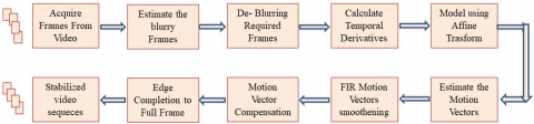
An efficient VS approach is proposed to stabilize the handheld camera videos. The proposed method De-blurs the video frames before estimating the motion vectors, which avoids inaccurate estimation and improves the stabilization efficiency. The VS experimental setup is given in Figure 3(a) and the complete VS procedure is summarized in Figure 3(b). Figure 3 demonstrates clearly that input video frames have inter-frame motion, which is intended to stabilize at the end processing. The Sony Handycam is used as a hand-held camera for the experiment to record real-time videos. The frames are grabbed, and frame pairs are processed, as shown in Figure 3(a).
The proposed method identifies the blurry frames present in the video sequences using the modified blurriness index based on the temporal derivatives as explained in section 4.1. After identifying the blurry frames with a significant amount of blur, the Wiener filter is used to De-blur identified blurry frames. The suggested VS method employs a hierarchical differential global motion estimation approach [5, 6] to assess inter-frame movement, as detailed in section 4.2. Unwanted camera movements are eliminated using an adaptive IIR filter, which is described in section 4.3. It is followed by Gaussian motion compensation and edge compensation in section 4.4 and 4.5 respectively to generate the full frame stabilized video.
(a) Experimental setup
(b) Detail VS procedure
Figure 3. Process of proposed VS methodology
4.1 Identification of blurry frames using the proposed blurriness index and de-blurring
The amount of blur present in the video sequences depends upon the various environmental conditions (scene or background) and different kinds of object motions. Thus, blurring does not uniformly present in all the frames of the video sequences. Usually, a sharper frame does not suffer from the large blur [8], but large objects with sharp edges are more affected by the motion blur. Thus, it is required to identify the blurry frames before de-blurring the video sequence.
4.1.1 Modified blurriness index
The VS technologies are employed for enhancing the quality of source videos by reducing blur and jitter thus producing videos that are pleasing to the human viewing system. Sophisticated digital cameras feature high-powered zoom lenses, which amplify undesirable camera movement. Unwanted motions are caused by slow and smooth hand motions. Jitters are quick and random handshakes that cause the entire scene to alter. In recent years, video stabilization has become an essential component of hand-held digital camera systems to improve their visual performance. This research aims to identify blurred frames within video sequences that are essential for video stabilization. The suggested method computes a new blurriness index by converting brightness for every pixel with the sum of squares of orthogonal temporal derivatives. The blurriness index calculated represents the enhanced foreground and background object motions. The proposed blurriness index is calculated for each ith frame using the derivative fx, and fy as:
$b_i=\sum_{x=1}^{{row }} \sum_{y=1}^{{col }} f(x, y, t) *\left(f_x(x, y, t)^2+f_y(x, y, t)^2\right)$ (15)
where, f(x, y, t) represents the brightness of p(x, y) pixel of the ith video frame.
The modified blurriness index can effectively identify the fine edge variations present because of camera motion within the foreground as well as the objects. Consequently, it can also represent the effect of object motion on the blurriness index. The employing of modified 4-point central difference derivatives for BI can represent a more precise and enhanced motion. The performance of the suggested blurriness index is compared to the performance of two generally used blurriness indexes based on the Inverse of the Sum of Square Gradients (ISSG) [7, 39], and the Blurriness index utilizing Image Gradients (BIG) [40].
The proposed method calculates the modified blurriness index using Eq. (15), for each frame. The blurriness index of each frame is compared with the threshold (Th) is defined as Th=mean(bi). If blurriness index bi<Th then the corresponding ith frame is identified as the blurry frame. Only the identified frames with significant blur will be De-blurred. The threshold Th is taken as the mean value since it is independent of the speed and direction of motions, and perform equally well in all type of motions.
De-blurring the blurry frames: The blind de-convolution is the most commonly used de-blurring method but it is computationally complex. Therefore, this paper proposes to implement the Wiener filter with reduced computational complexity and better acceptable restoration results. Wiener filter is a minimum mean square error (MSE) filter that employs a linear De-convolution method [10]. Thus it is computationally less intensive. But it gives poorer results in the presence of noise. The filter is designed by minimizing the estimated MSE between the original frame f(x,y,t) and its estimate $f^{\wedge}(x, y, t)$ by using the Wiener filter defined by Bojarczak and Lukasik [37]. However, sometime de-blurring would cause some ringing effects in the de-blurred frame caused by the high-frequency drop-off. Thus, in addition, the function that is used to solve this problem is edge-taper. Edge-tapering blur the edges of the input frame slightly, before applying the de-convolution thus reducing the ringing effects.
4.2 Global ME via hierarchical differential motion
The study introduced a layered approach to motion estimation for analyzing changes between successive video frames. This hierarchical method's core concept involves evaluating motion at a reduced resolution, which helps mitigate aliasing effects. The technique employs a Gaussian pyramid with L=3 levels [6] and is built over a pair of frames, f(x,y,t) and f(x,y,t-1). The movement of two consecutive frames f(x,y,t) and f(x,y,t-1) is represented using a six-parameter affine transformation [6, 18, 33], which is expressed as:
$\begin{gathered}f(x, y, t)=f\left(\mathrm{~m}_1 \mathrm{x}+\mathrm{m}_2 \mathrm{y}+\mathrm{m}_5, \mathrm{~m}_3 \mathrm{x}+\mathrm{m}_4 \mathrm{y}+\mathrm{m}_6, t\right. \\ -1)\end{gathered}$ (16)
where, m1, m2, and m3, m4 form 2×2 affine matrix A, and m5, m6 are translation vector $\bar{T}$ as:
$\mathrm{A}=\left(\begin{array}{ll}m_1 & m_2 \\ m_3 & m_4\end{array}\right)$, and $\bar{T}=\binom{m_5}{m_6}$ (17)
The following quadratic error function has to minimize to estimate the affine parameters.
$\begin{gathered}\mathrm{E}(\mathrm{m})=\sum_{\mathrm{x}, \mathrm{y} \in \Omega}\left[\mathrm{f}(\mathrm{x}, \mathrm{y}, \mathrm{t})-\mathrm{f}\left(\mathrm{m}_1 \mathrm{x}+\mathrm{m}_2 \mathrm{y}+m_5, \mathrm{~m}_3 \mathrm{x}\right.\right. \left.\left.+\mathrm{m}_4 \mathrm{y}+\mathrm{m}_6, \mathrm{t}-1\right)\right]^2\end{gathered}$ (18)
Using the Taylor series expansion technique outlined by Hany Farid in studies [6, 18], the motion vectors are determined through differential global motion estimation. The only modification is that the temporal derivatives are calculated using the Barron method [13]. The derivatives in the x and y direction are given in Eqs. (12)-(13), and the time derivative is given by:
$\begin{aligned} f_t(x, y, t)= & \operatorname{conv}((f(x, y, t-1) *[0.25\ 0 .25])+ (f(x, y, t) *-[0.25\ 0 .25]))\end{aligned}$ (19)
The estimated global motion vectors calculated for each pair of frames are represented as:
$\operatorname{GMV}(\mathrm{t})=\left\{\mathrm{GMV}^{\mathrm{x}}(\mathrm{t}), \mathrm{GMV}^{\mathrm{y}}(\mathrm{t})\right\}=\overline{\mathrm{T}}=\left\{\mathrm{m}_5, \mathrm{~m}_6\right\}$
where, GMVx(t)=m5 is a translation in the x direction and GMVy(t)=m6, is the translation in the y direction. The rotation and scaling parameters matrix are set as $A=\left[\begin{array}{ll}m_1 & m_2 \\ m_3 & m_4\end{array}\right]$. These parameters represent undesired motions in video sequences. If the length of a video sequence is large then the error due to accumulation of global motion vectors also increases. This causes missing frame areas and thus loss of information. Hence, the motion-smoothing method is required to remove the undesired motions, which minimizes the missing frame areas.
4.3 Motion smoothing
Researchers have developed numerous techniques to reduce unwanted camera movements. However, most of these approaches were either computationally intensive or only effective for basic and slow camera motions. Their performance diminishes when dealing with substantial objects and camera movements, particularly in handheld mobile video recordings. Consequently, there is a need to efficiently minimize jitters and the calculated accumulated global motion vectors $A G M V(t)$. The proposed approach employs a first-order adaptive IIR filter [9] to smooth out accumulation errors. This IIR filter was chosen for motion smoothing primarily due to its straightforward implementation and effectiveness.in systems that operate in real time and consume less memory. The combined vectors of global motion $A G M V(t)$ are calculated from estimated motion vectors, as:
$A G M V(t)=\sum_{i=2}^t G M V(t-1)+G M V(t)$ (20)
where, AGMV(t) is represented as:
$A G M V(t)=\left\{A G M V^x(t), A G M V^y(t)\right\}$ (21a)
To obtain the smoothed accumulated motion vectors, implement a first-order IIR filter on Eq. (21). This can be expressed as:
$\begin{gathered}\operatorname{ASM}(\mathrm{t})=\tau * \operatorname{ASMV}(\mathrm{t}-1)+(1-\tau) \\ * \operatorname{AGMV}(\mathrm{t}-1)\end{gathered}$ (21b)
In this context, $A G M V(t)$ which represents the cumulative smoothed motion vectors, is defined as follows:
$\operatorname{ASMV}(\mathrm{t})=\left\{\operatorname{ASMV}^{\mathrm{x}}(\mathrm{t}), \operatorname{ASMV}^{\mathrm{y}}(\mathrm{t})\right\}$ (22)
where, $\tau$ is defined as a smoothing parameter that generally ranges between 0≤τ≤1. for the Paresh et al. [19] $\tau$ is set to 0.96 since it is the uppermost limit.
4.3.1 Proposed FIR filter design
The comparative smoothened motions produced by the FIR filter are satisfactory and pleasant to the human visual system. FIR filters might hold several advantages against IIR filters while it comes to motion smoothing as:
Guaranteed Stability: Because FIR filters are inherently stable, their output won't increase uncontrollably. This is important because unstable filters might result in undesired distortions as well as artifacts while processing videos.
Phase Response: A linear phase response is a possible design for FIR filters. This implies that the delay experienced by each frequency component is the same, which is crucial for maintaining the temporal links between various video signal components. This corresponds to smoother transitions as well as prevents the introduction of jerky movements as a result of phase shifts in motion smoothing.
Filter depends on the current and past four frames motion vectors. Frames are filtered with filter coefficients b0=2-1, b1=2-2, b2=2-3, b3=2-4, and b4==2-4. The quantity of previous frames can be adjusted as necessary, with corresponding modifications to the coefficients. The filtering process is executed as:
$B M V_{\text {filter }}(n, b l k)=\sum_{\mathrm{K}=0}^{\mathrm{d}} \mathrm{b}_{\mathrm{k}} * B M V_{\text {old }}(n-k, b l k)$ (23)
This paper has proposed using the lower order fast FIR filter design with the filtered numerator coefficient vector $b$=0.2 with denominator coefficient vector normalized to a=1. The proposed method of FIR filter smoothens and stabilizes the motion better. Uses of FIR filter almost eliminates the requirement of compensation stage. However, FIR filter needs more computation and memory as limitations. Thus, it is concluded that FIR filters are a suitable alternative for motion smoothing where stability, linear phase response, with economy of design are priorities.
4.4 Warping and motion compensation
In the stabilization algorithm, the warping technique aligns a newly received frame with the positions of the preceding frame. Substantial movements are detected at the coarse level through warping, utilizing Bi-cubic interpolation. This process is then refined iteratively across each level of the pyramid. When the calculated motion vectors at a specific pyramid level L are m1, m2, m3, m4, and m5, m6, the estimated affine matrix A should be used to warp the original frame, along with the smoothened global translation vector $\bar{T}$ given as:
$A=\left[\begin{array}{ll}m_1 & m_2 \\ m_3 & m_4\end{array}\right]$. and $\bar{T}=\binom{2^{L-1} m_5}{2^{L-1} m_6}$ (24)
Upon completing each level of the pyramid, it will be necessary to repeatedly transform the initial frame using the motion calculated at every pyramid stage. Two affine matrices A1 and A2 with their corresponding translation vectors T1 and T2 are combined as:
$A=A_1 A_2$ and $\bar{T}=A_2 T_1+T_2$ (25)
The use of a hierarchical pyramid approach with Bi-cubic interpolation for warping improves the stabilization performance under large objects and camera motion. The paper proposed to use the GKF [9, 31] for motion compensation because they are simple to implement. The standard deviation is set to $\sigma=\sqrt{k}$ [9] where k is the kernel parameter or the size of the neighborhood. The value of the kernel parameter k must not exceed 6. Employing GKF helps reduce areas with missing frames. The compensated motion transformation between frames i and j in a video sequence is determined using the following calculation:
$C_t=\sum_{i \in N_t} T_j^i * G(k)$ (26)
where, G(k) the GKF, is referred to by Matsushita et al. [9], and Nt, is a set of neighboring frames given as Nt=m: k-n≤m≤k+n. The compensated motion frames $f_t^{\prime}$ can be warped from the original frame ft by:
$f_t^{\prime}(x, y, t)=C_t * f_t(x, y, t)$ (27)
4.5 Edge completion
Despite motion smoothing, some areas of missing frames persist due to cumulative errors and rotational effects. The proposed approach achieves seamless stitching of these missing frame regions by employing a simplified edge completion technique [12]. This method bears a slight resemblance to the edge completion approach described by Matsushita et al. [9]. It utilizes the surrounding present frames to fill in the areas where frames are missing:
$f_k(i, j)={median}\left[f_N(i, j)\right]$ (28a)
$N \in[(k-n, . ., k+n]$ (28b)
where, k is the number of currents is frames, and n is the integer. The application of Gaussian motion compensation effectively reduces the areas that are missing, making it possible to use small values like 3 or 5 for n in Eq. (28) to successfully fill in these gaps.
The proposed VS method is developed using MATLAB software on a Core 2 Duo 2.4 GHz processor. Database is represented in Section 5.1. Then Section 5.2 compares the performances of the two commonly used blurriness indexes with the proposed method. De-blurring video before motion estimation improves the stabilization quality as explained in section 5.2.2. Outcomes of performance comparison of different temporal derivatives are given in section 5.3. Th results of motion smoothing and compensation are presented in the section 5.4, Two case studies are presented in the section 5.5 and 5.6 respectively for large object motion (in 5.5) and for video resize attack (in 5.6). The process of edge completion produces fully stabilized video sequences that span the entire frame.
The results are presented in mainly three stages. In the first part, the results of the modified blurriness index-based estimation and VS are considered. The second part compares the effectiveness of different motion smoothing techniques using quantitative analysis. Subsequently, the paper presents the step-by-step outcomes of the proposed VS approach, which includes edge completion. Overall, this research has advanced the creation of visually coherent full-frame videos from unprocessed input data.
5.1 Input data
Real-time video sequences with a resolution of 176 × 144 at 15 fps are generated using Nokia (6303) cell phones and a Sony DCR SX45 digital camcorder fps (frames per second), and 720 × 576 at 25 fps respectively. The videos with the camcorder are resized the image was resized to 176 × 144 to decrease processing time, as shown in Figure 4. Effectiveness of the VS algorithm was evaluated using 32 real-time video samples, covering five categories of camera and object movements. Five distinct videos one for each category are used for the statistical evaluation in the paper as in Figure 4. Video considered for evaluation is taken from references as well as in real-time true captured videos with different motions of objects six different cases of motions are considered for the evaluation. Paper presented the results and study for blurriness index-based VS for different kinds of object motions using quantitative and qualitative evaluation.
|
Category |
Videos |
|
|
Moving Away |
Moving Towards |
|
|
Both the camera and the object both are moving with speed >= 10 m per sec |
||
|
Both the camera and the object both are moving with speed < 2 m per sec |
||
|
Camera moving with speed < 2 m/s Object Stationary |
||
|
Camera stationary Large Object is moving with speed > 10 m/s |
||
|
Camera stationary but object moving with speed < 2 m per sec |
||
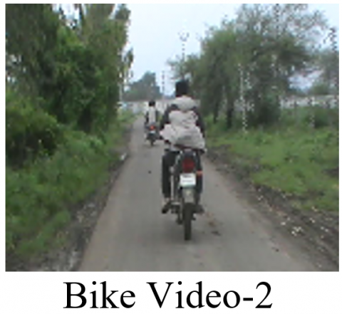
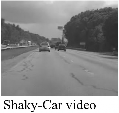
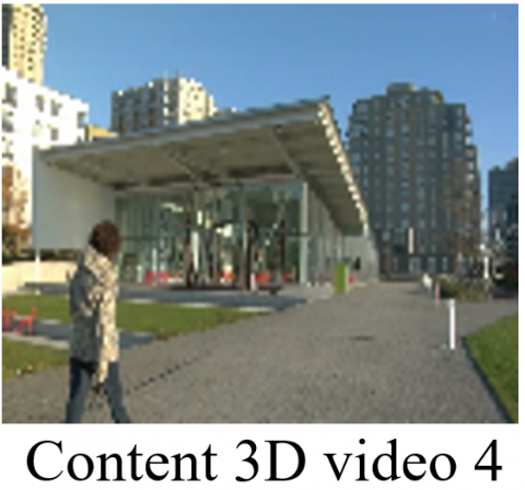
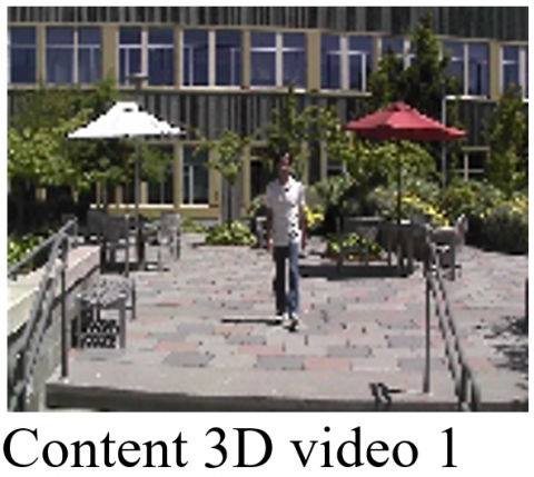
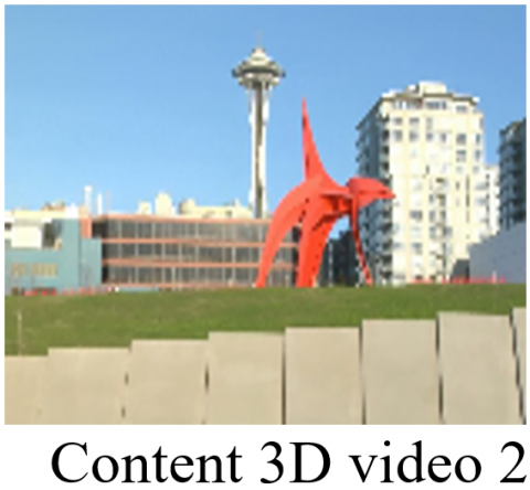
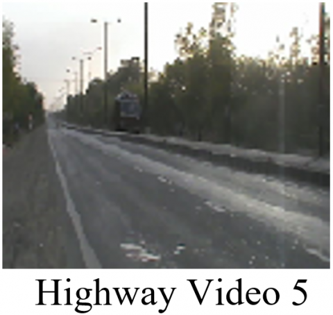
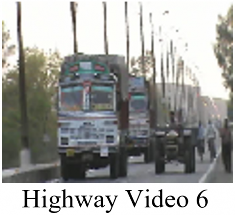
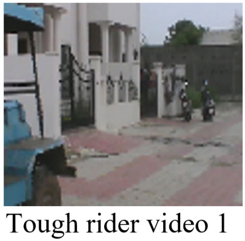
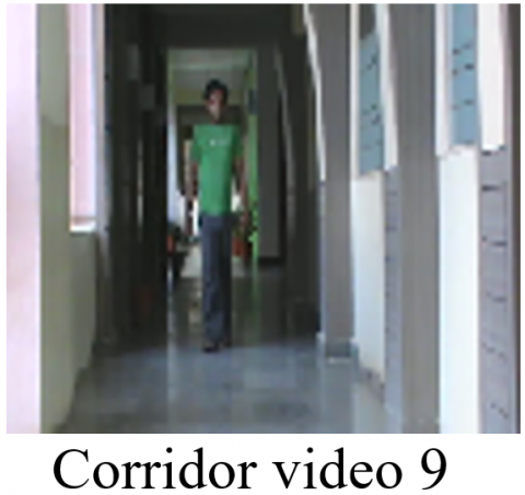
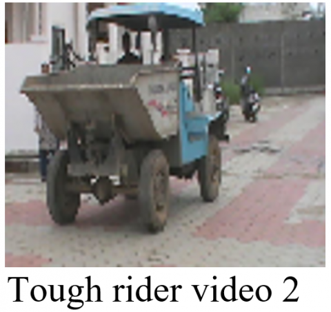
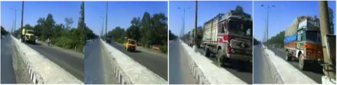
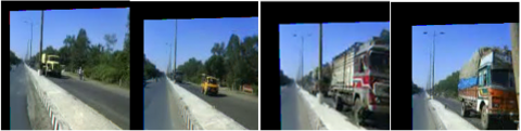
Figure 4. Input video categories a) Highway Video 2, b) Highway Video 6, c) Tough rider Video 2, d) Content 3D video 4, e) Content 3D video 2 [7]
5.2 Performance comparison of blurriness indexes
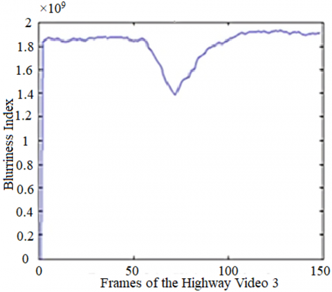
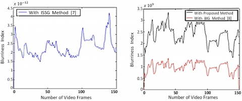
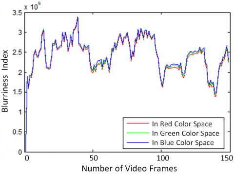
This section compares the suggested blurriness index with blurriness indexes used by the Shen ISSG method [38] and Manish BIG method [39] as in Figure 5. The fast object motion is considered and the videos are taken in real-time from the highway containing the incoming and outgoing object in frames. As experimentation, the blurriness index is calculated in the RGB domain for impact identification as shown in Figure 5.
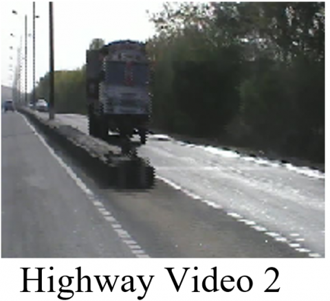
Figure 5a) and b) show that the red color space has the least amount of influence and value of the blurriness index and is thus considered for further evaluation in this paper. The Blurriness index of the ISSG is very small, as it is the inverse of the sum of the square gradient measure. Thus, it is not possible to represent it with the other two blurriness indexes together, thus shown separately side by side. The results show that the blurriness index of Highway Video 2 has many fluctuations due to camera motion, as in Figure 5(a). But because the camera is stationary in the case of Highway Video 6, there are fewer variations in the blurriness index, as is clear from Figure 5(b). The blurriness index of the ISSG method is relatively smoother. It can be observed that the amount of blur in the video depends on the kind of object and camera motions. The quantitative average value of the BI calculated as in Figure 5, is given in Table 1. It is clear thet the proposed modified BI (MBI) offers significant magnitude improvement over the other two BI and thus represents the motion better.
When the object is moving toward the camera, the blurriness index is increased, and when the object moves away from the camera or leaves the scene, the blurriness index is decreased. The proposed method uses the 4-point central difference to calculate the blur index and hence represents the enhanced blur index. Thus, the object motion is much more clearly represented by the proposed method than by the previous two methods. The proposed VS method is also capable of identifying the stationary and blurry background objects better than the gradient method.
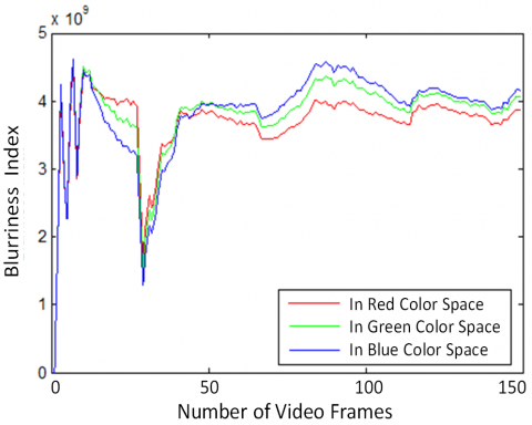
The Blurriness index is individually calculated for R, G, and B, each color space, using the proposed method to observe the effect of blurring on tri-color space, as compared in Figure 6. Although the amount of blur is different in each color space, the nature of the blurriness index remains the same for each color space. Thus, any one of the color spaces can be used to calculate the blurriness index, and this will reduce the computation cost.
It is clear from Figure 6 that the blur affects each color space separately. The blurriness index bi is only calculated for the red color space using the (15) by comparing it with the threshold Th. Only the frames having a blurriness index less than a threshold are deblurred.
(a) Blurriness index for video Highway Video 2
(b) Blurriness index for video Highway Video 6
Figure 5. Comparison of the blurriness index for Highway Videos with large object motion
(a) Blurriness index for Highway Video 6
(b) Blurriness indexes for Highway Video 2
Figure 6. Comparison of blurriness index for RGB try color space
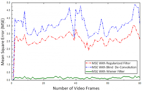
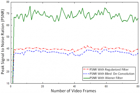
5.2.1 Performance evaluation of de-blurring methods
In this section performance of various de-blurring methods is compared based on MSE and peak signal-to-noise ratio (PSNR).
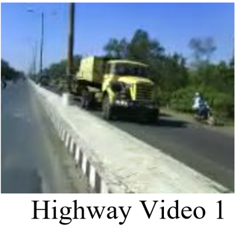
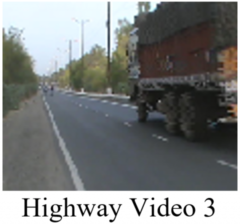
The results of MSE and PSNR are shown in Figure 7 and Figure 8, respectively, for video deblurring for distinct Highway Videos in the scene. Highway Video 1 with multiple moving objects, with the fast object moving towards the camera, is considered for evaluation.
The MSE is the performance measure used for evaluating the deblurring effectiveness and is defined as:
$M S E-\left(\frac{1}{M N} \sum_{\mathrm{x}=1}^{\mathrm{M}} \sum_{\mathrm{y}=1}^{\mathrm{N}}\left(f_1(x, y)-f_2(x, y)\right)^2\right)$ (29)
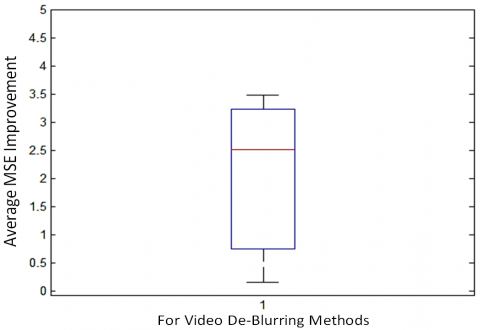
It can be concluded from Figures 7 and 8 that the MSE is minimum for the Wiener filter method compared to that of the regularized and blind methods. The box plot comparison for the MSE and the PSNR for deblurring methods is presented in Figure 8(b) and Figure 8(c), respectively.
It can be observed from the parametric comparisons from Table 2 and Figure 8 that the proposed Wiener filter method offers a significant 60% improvement in PSNR and minimizes MSE performance, achieving as 0.1634 by the wiener filter and offering 21 times improvement over the regularized filter approach and 15 times improvement over blind deconvolution approach. Thus, in this paper, it is proposed to deblur the frames using a Wiener filter and then stabilized them.
Table 1. Average BI value for the Highway Video 6
|
Parameter |
With BIG [38] |
With ISSG [39] |
Proposed MBI |
|
Blurriness Indexes |
1.6723 |
1.5623 |
3.462 |
Table 2. Average parametric comparison of deblurring methods for Highway Video 1 for 75 frames
|
Parameters |
Regularized Filter |
Blind Convolution |
Wiener Filter |
|
Average MSE |
3.48234 |
2.5246 |
0.1634 |
|
Average PSNR |
40.02456 |
36.2134 |
68.6234 |
Figure 7. Comparison of MSE for various de-blurring methods for Highway Video 1
(a) Comparison of PSNR for de blurring methods for Highway Video 1
(b) MSE improvement box plot
(c) PSNR improvement box plot
Figure 8. Comparison of PSNR for various deblurring methods for Highway Video 1
Table 3. Percentage of blurry frames with proposed mean and median blurriness threshold
|
Category |
Video Name |
Number of Video Frames |
Object Size |
Mean Blur Index |
Median Blur Index |
Percentage of De-Blurred Frames with Median Index |
Percentage of De-Blurred Frames with Mean Index |
|
Category I |
Highway Video 2 |
150 |
Large |
2.4008 |
2.462 |
49% |
45% |
|
Category II |
Content 3D video 4 |
300 |
Small |
2.3427 |
2.3278 |
49.5% |
52.84% |
|
Category III |
Content 3D video 2 |
300 |
Small |
3.3603 |
3.3566 |
49.5% |
57.2% |
|
Category IV |
Highway Video 6 |
180 |
Large |
3.7387 |
3.8 |
49.24% |
32.66% |
|
Category V |
Tough Rider video 2 |
300 |
Large |
2.1346 |
2.0100 |
49.54% |
55% |
5.2.2 Identifying blurry frames
The characteristics of temporal derivatives are influenced by various factors in a video sequence, including the background scenery, the types of objects in motion, and the quantity of moving elements. As a result, the temporal derivatives calculated along the x and y axes differ for each distinct category of video footage. If the blurriness index is less than the threshold Th, then the corresponding frame is identified as a blurry frame. The threshold Th of the blurriness index is also different for each video.
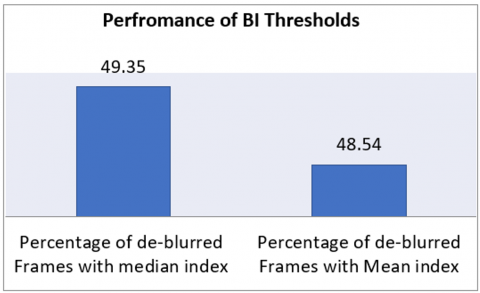
Figure 9. Performance comparison of the BI median and mean thresholds
Thus, it is desired to set up a common criterion for choosing the threshold Th, which is independent of motion and video type. In the proposed method, the threshold Th is set to the mean value of the blurriness index bi. Because the mean index performs better with different categories of motions. Since the mean value is the best possible nearest value to the maximum frequency in the blurriness index histogram. The outcome and comparison of the blurriness index selection using mean and median thresholds are given on Table 3.
It can be observed that the median blurriness index threshold (Th) is selected as it offers higher percentage of frames to be deblurred. The performance comparisons of the overall frames deblurred by two BI thresholds as the experiments are shown in Figure 9. It can be observed that the Mean value as a threshold may offer better performance.
5.3 Stabilized video comparison with different temporal derivatives
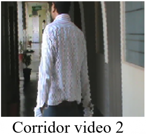
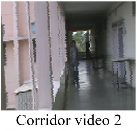
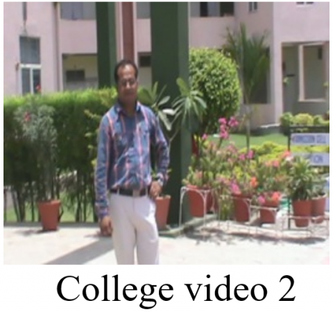
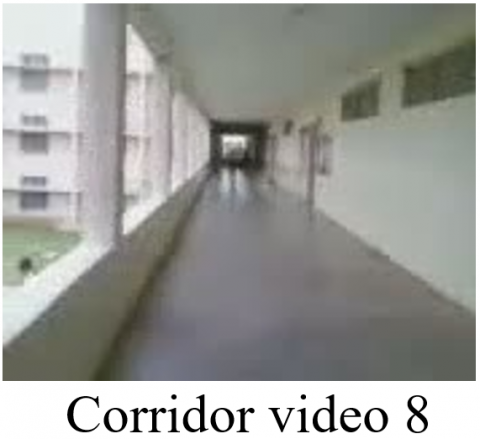
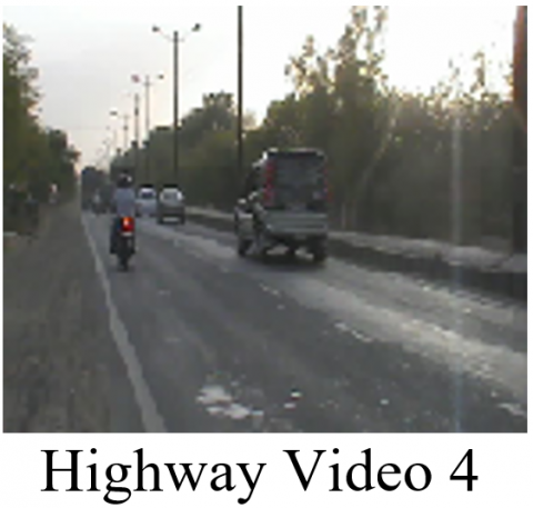
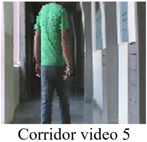
The effectiveness of VS system is contingent upon the accuracy of the motion estimation. The proposed method employs differential global motion estimation, which utilizes temporal derivatives. Consequently, the precision of motion estimation is directly influenced by the quality of temporal derivatives. To assess the performance of the proposed stabilization technique, the Inter Transformed Fidelity (ITF) was computed and compared using various temporal derivative methods. These include simple pixel differences, two-point central differences, 1D separable filter, and four-point central differences, as outlined in the study by Rawat and Singhai [19]. The research provides an extension of the ITF comparison as referred by Rawat and Singhai [7]. The comparison of ITF for stabilized videos using various spatial-temporal derivatives for our proposed VS method is presented in Table 4. Among all methods, two-point central derivatives yield the lowest ITF. For some videos, such as Corridor video 5 and Highway Video 5, the simple pixel difference method results in an ITF lower than the original.
Table 4 demonstrates that the proposed method is more effective when scene objects, particularly those in the background, are distant from the camera.
Table 4. ITF comparison for videos [7] that have been stabilized using various temporal derivatives
|
Category |
Video Name |
Inter-Frame Transformation Fidelity (ITF) with |
||||
|
For Original Video |
With Simple Pixel Difference Derivatives |
With Two-Point Central Difference Derivatives |
With 1D Separable Filter Derivatives |
With Four-Point Central Difference Derivatives |
||
|
Camera and the object are moving with speed >= 10 m per sec |
Bike video2 |
24.335 |
26.0849 |
24.8447 |
26.3397 |
26.3625 |
|
Shaky car |
17.8641 |
18.9170 |
18.7351 |
19.4042 |
19.4955 |
|
|
Highway Video 1 |
14.4538 |
15.2979 |
14.9124 |
15.2832 |
15.2886 |
|
|
Highway Video 2 |
18.248 |
19.3922 |
18.7961 |
19.4664 |
19.4401 |
|
|
Camera and the object are moving at speed < 2 m per sec |
Corridor video 2 |
19.441 |
20.6010 |
19.8795 |
20.6525 |
20.2357 |
|
Content 3D video 4 |
20.0309 |
21.8754 |
20.7864 |
22.2513 |
22.4446 |
|
|
Corridor video 3 |
25.5852 |
27.2563 |
26.2849 |
27.2807 |
27.3182 |
|
|
Content 3D video 1 |
16.2031 |
16.9573 |
16.4117 |
17.6431 |
18.0605 |
|
|
Camera moving at < 2 m per sec and object stationary |
College video 2 |
21.3671 |
22.9163 |
21.7235 |
23.2452 |
23.0745 |
|
CRO video 6 |
23.1706 |
24.5036 |
22.7955 |
24.8527 |
24.6484 |
|
|
Corridor video 8 |
20.6443 |
21.4517 |
21.0644 |
21.5291 |
21.5239 |
|
|
Content 3D video 2 |
18.7910 |
20.1670 |
19.5477 |
20.0787 |
20.2585 |
|
|
Camera stationary Large Object is moving with speed > 10 m/s |
Highway Video 3 |
33.1828 |
34.4618 |
32.4787 |
35.9676 |
36.0688 |
|
Highway Video 4 |
30.1324 |
31.5641 |
31.1320 |
31.8283 |
31.8326 |
|
|
Highway Video 5 |
43.4356 |
39.1720 |
40.7624 |
41.5970 |
43.5636 |
|
|
Highway Video 6 |
20.6238 |
22.5872 |
21.3792 |
22.5510 |
22.6719 |
|
|
Camera stationary Object is moving with speed < 2 m/s |
Corridor video 5 |
34.0159 |
33.6929 |
34.0353 |
35.3158 |
34.9858 |
|
Tough Rider video 1 |
30.4865 |
31.0122 |
29.5536 |
32.1590 |
32.1164 |
|
|
Corridor video 9 |
39.3615 |
36.2835 |
32.1169 |
40.8011 |
40.4933 |
|
|
Tough Rider video 2 |
28.8044 |
30.2917 |
28.0155 |
30.8369 |
30.428 |
|
This is evident in cases like Bike Video 2 and Shaky Car video. The suggested four-point central difference-based derivatives show superior performance in videos featuring large and rapid object motion, as seen in category four, and in scenes with multiple moving objects, such as Highway Video 6 and Highway Video 2. However, the method's effectiveness is less pronounced when the camera is stationery and objects move slowly (speed < 2 m/s), as in category five, or when objects are in close proximity to the camera. While the 1D separable filter method produces a marginally better ITF, the proposed approach achieves comparable results.
5.4 Result of motion smoothing and compensation
In this section, the performance of various motion, and smoothing methods are compared based on estimated X and Y translations. Since blue space is having higher translation thus for the performance comparison translation is plotted for blue color space.
5.4.1 Comparison of translation with various motion smoothing methods
For comparison of smoothing performance, the estimated accumulated X and Y translations using our proposed hierarchical differential global motion estimation methods are smoothened by different smoothing methods in Figures 10-13.
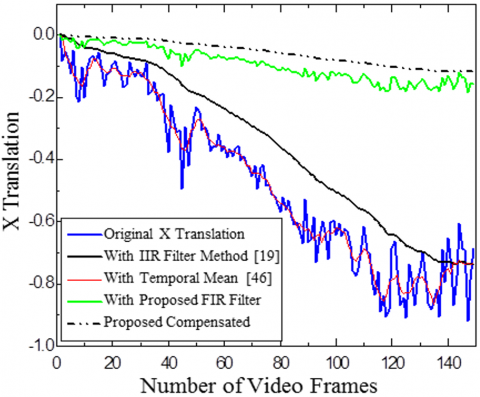
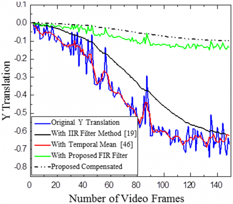
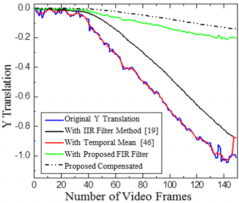
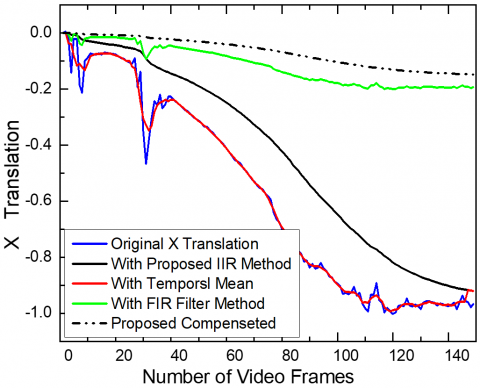
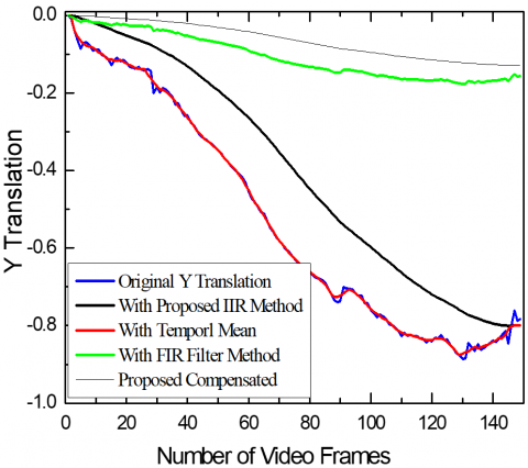
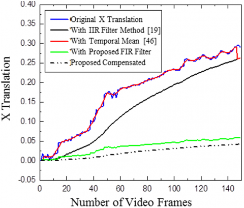
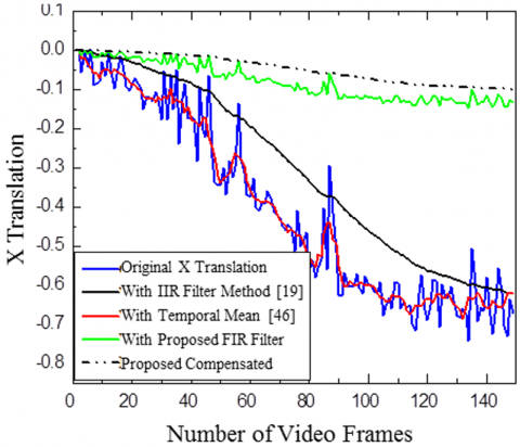
Highway Video 2 is shown in Figure 10 and Figure 11. The proposed adaptive IIR filter with α=0.96 is employed to refine the estimated X and Y translations. A Gaussian kernel filter with β=0.8 is utilized for motion compensation. This approach effectively mitigates unwanted movements, resulting in video stabilization.
Figure 10. Comparison of smoothing X and Y translation with various motion smoothing methods for Highway Video 1
Figure 11. Comparison of smoothing X and Y translation for various motion smoothing methods of Highway Video 2
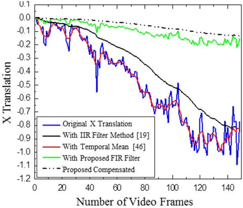
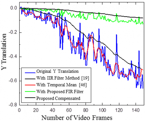
Comparison of X and Y translation for Highway Video 1 and effectiveness of the suggested approach is evaluated against a temporal mean filter [7] and 1IR filter [19]. Both the video used in Figures 10 and 11 belong to category one with the camera and object both are moving. The results indicate that the suggested FIR filter technique effectively smooth’s and stabilizes the motion. Uses of FIR filter almost eliminate the requirement of compensation stage.
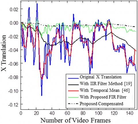
Figure 12 and Figure 13 respectively show the comparison of X and Y translation for CRO video 6 and Content 3D video 4. These videos have stationary backgrounds or objects with the camera slowly moving forward. Thus most of the motion is in the X direction
Quality of stabilization with the proposed FIR filter can be seen from the X translation in Figure 14 and Figure 15 show a comparison of X and Y translations for Highway Video 6 and Tough rider video 2. The IIR filter gives better smoothing thus estimating the jitters better.
Figure 12. Comparison of smoothing X and Y translation with various motion smoothing methods for CRO video 6
Figure 13. Comparison of smoothing X and Y translation with various motion smoothing methods for content 3D video 4
Figure 14. Comparison of smoothing X and Y translation for various motion smoothing methods of Highway Video 6
5.4.2 Result of motion smoothing and compensation
The performance of stabilized video using the proposed blurriness index is compared with the blur index used in some studies [38, 39], respectively. A first-order adaptive to stabilize the video, and an IIR filter is employed to smooth the estimated translations along the X and Y axes.
(a) For Highway Video 2
(b) For Highway Video 6
Figure 16. Comparison of the smoothened X and Y translation for different blurriness indexes
Table 5. Comparison of ITF for stabilized videos with different blurriness indexes
|
Category |
Video Name |
Inter-Frame Transformation Fidelity (ITF) |
|||
|
Original Video |
Blurriness Index of ISSG [7] |
Blurriness Index of BIG [8] |
Proposed Blurriness Index |
||
|
Category I |
Highway Video 2 |
18.1423 |
18.828 |
19..08 |
19.074 |
|
Category II |
Content 3D video 4 |
16.076 |
18.112 |
17.4285 |
18.5886 |
|
Category III |
Content 3D video 2 |
9.52547 |
9.5666 |
9.5667 |
10.2297 |
|
Category IV |
Highway Video 6 |
10.1703 |
10.4506 |
10.8959 |
10.9917 |
|
Category V |
Tough Rider video 2 |
14.3628 |
14.6558 |
14.6575 |
14.6566 |
The results of smoothened X and Y translations of Highway Videos 2 and 6 are compared for various blurriness indexes and compensated translation after Gaussian Kernel filtering for the proposed method is also shown as in Figure 16. The proposed method gives better smoothened and stabilized translation results.
To objectively assess the performance of various methods compared to the proposed approach, the Inter-frame Transformation Fidelity (ITF) [12] is computed. This metric measures the PSNR between consecutive frames. The ITF can be defined mathematically as:
$\operatorname{ITF}=\frac{1}{N_{\text {frame }}-1} \sum_{j=1}^{N_{\text {frame }}-1} \operatorname{PSNRR}\left(f_j, f_{j+1}\right)$ (30)
where, Nframe is the number of total frames in the videos, PSNR is defined as the PSNR calculated for each pair of frames as:
$\operatorname{PSNR}=10 \log \left(\sum_{\mathrm{x}=1}^{\mathrm{M}} \sum_{\mathrm{y}=1}^{\mathrm{N}} \frac{f_t(x, y)^2}{\left(f_t(x, y)-f_{(t-1}(x, y)\right)^2}\right)$ (31)
The comparison of ITF for videos stabilized under varying levels of blurriness is presented in Table 5. In the majority of scenarios, the suggested approach demonstrates superior performance. As the level of blurriness intensifies, the effectiveness of the proposed method also shows improvement.
5.4.3 State of art comparison
The T – test is performed to justify the performance comparison with stat of art methods in the paper as illustrated in the Figure 17. It is clear from the Figure that the ITF has significant improvement. It can be observed from the Figure that proposed MBI offers the 2.69% average ITF improvement over ISSG [39] based BI approach, while compared to BIG [40] approach, the proposed MBI offers the 11.9% ITF improvement on an average.
Similarly of the ITF for VS with state of art temporal derivatives methods based on the T – test are compared as shown in the Figure 18. The temporal derivatives used by the Rawat and Singhai [7] have been compared with the proposed 4 point central derivative method for VS.
Figure 17. Result of the ITF for VS with state of art BI measures methods using T – test
Figure 18. Result of the ITF for VS with state of art temporal derivatives methods based on the T – test
It is clearly observed from Figure 18 that proposed method offers 0.23 % ITF improvement over Farid and Woodward [8] 1D separable filters, while on 2 point derivative approach proposed method offers 7.02% average ITF improvement. Also improvement of 3.075% is observed on average over the simple pixel derivative based VS approach.
During the next experiment the rest of the VS system is kept same as proposed approach but derivatives are modified with proposed FIR filter in place of IIR filter. The modified and simple edge completion method is adopted for the full frame video generation. The Qualitative results are presented for the different frame size the kind of fast object motion.
5.5 Case studies under large object motion
In this section for better observations, some specific cases of original and stabilized frames with the proposed method are compared for the frames with large objects or higher motion. It can be observed from the Figure 19 as above that generates full-frame stabilized frames with better depth and edge representations.
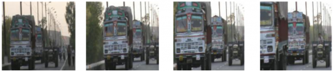
(a) Five consecutive frames of Highway Video 1 from 34 to 38
(b) Stabilized results of designed method with our proposed approach
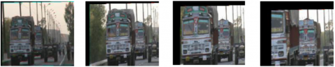
(c) Five consecutive frames of Highway Video 1 from 84 to 88
(d) Stabilized results with our proposed method
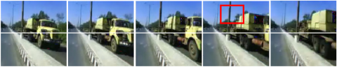
Figure 19. Results of proposed VS method comparison for stabilized Highway Video 1
The stabilization quality can be compared for five consecutive frames 34-38 in Figure 19 (a) and (b). It can be seen that the object in the truck is better visible in stabilized video frame as shown in the red square. The quality of the stabilized rotation can be observed by the pillar in Figure 19 (c) and Figure 19 (d). The Highway Video depicted in Figure 19 contains large, rapidly moving objects throughout the scene. This leads to numerous frames susceptible to blurring effects. The proposed method has effectively addressed this issue by producing stable and visually appealing frames.
5.6 Case study of resize attack on VS
Figure 20(a) and (b) illustrate the X and Y translations for Highway Video 1 at two alternative frame sizes of [174×176] and [256×256], respectively. The translation is calculated for various frame sizes using our proposed video stabilization approach.
The proposed "Compensated" approach produces the smoothest outcomes with the lowest total translation values. Figure points out better video processing quality and stability.
A systematic result of the proposed VS method for the distinct Highway Video 6 is shown in Figure 21. Each 25th frame of the input video sequence is shown in Figure 21(a). The large accumulation error after the estimation is present at the top of the frames, which generally increases with the number of video frames shown in Figure 21(b).
The proposed motion smoothing technique effectively mitigates the accumulation error, resulting in a reduction of missing frame areas as illustrated in Figure 21(c). Finally, the edge completion method fills up the missing frame areas to generate full-frame stabilized video as in Figure 21(d).
Similarly, Figure 22 shows the result of the proposed VS method for distinct Highway Video 1 from category I, with the fast-moving object. It can be observed from Figure 22 that if video frames are resized then X and Y translations are increased when the frame size is increased. Since resized frames have increased blur thus, the estimated motion is different for different resolutions.
The video with rolling shutter effects is the sixth input category of the video. One common case of the rolling shutter video is used by Liu et al. [3].
(a) Smoothen X Translation for Highway Video 1 for [174×176] and [256×256] frame sizes
(b) Smoothen Y Translation for Highway Video 1 for [174×176] and [256×256] frame sizes
Figure 20. X and Y translations for the different frame sizes of Highway Video 1
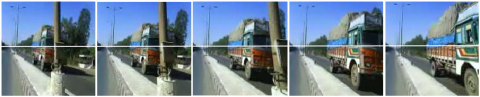
a) Every 25th frame of the original video sequence
b) Estimated frames with large accumulation error
c) Smoothen video frame sequence
d) Edge Completed full frame stabilized video sequences
Figure 21. Stage-wise results of the proposed stabilization method for Highway Video 6
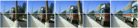
Figure 22. Results of the suggested stabilizing technique, broken down per stage for Highway Video 6 top row: Every 25th frame of the original video sequence. Second row: estimated frames with large accumulation error. Third row: filtered video frame sequence. Last row: edge completed full frame stabilized video sequence
Guilluy et al. [43] have presented a comprehensive survey of video stabilization technologies. The primary goal of this contribution is to provide answers to such issues as well as a sufficiently integrative paradigm to offer a greater awareness of the advancement of this research field, which has significant academic and industrial significance. The main problems, practical issues, and mathematical core principles of VS algorithms are discussed in this work. VS is being revolutionized by AI and deep learning techniques can be investigated by researchers as a means of improving the analysis and compensation of intricate camera motions, particularly in difficult situations including rapid movements or obstacles.
Recently, Zhao et al. [44] have presented the use of the iterative optimization algorithm to improve the efficiency of the VS systems for hand held devices for full frame video generation. The study of the roll and panning is also the open field of research. It is also point of interest in future to consider the depth of field for analysis. VS has been introduced by Souza et al. [45] with a succinct physical interpretation.
An effective VS algorithm method for videos taken with a handheld camera is suggested in the paper. The video sequence should be de-blurred first, and then the global motion parameters should be estimated. The use of 4-point temporal derivatives is proposed to create a new blurriness index. The proposed approach to identify the blurry video frame uses the mean blurriness index as a threshold. Differential motion estimation is utilized to estimate motion vectors, and an adaptive FIR filter is employed to smooth them. The frames are warped using bi-cubic interpolation at each pyramidal level, which increases the effectiveness of the direct technique. The suggested strategy results in better stabilized X and Y translation.
The proposed method offers the best average ITF with blurriness index performance or average ITF of 13.65537 for original videos, and compared with average ITF of studies [7, 8] and proposed respectively as 14.3226, 13.13715, 14.70812 and proposed method offer the best. The improvement in ITF represents the contribution of research. The proposed method compares the performance of three de-blurring methods and it is clear the proposed method of Wiener filter offers the minimum MSE and maximum PSNR.
Performance of state of art BI measures is compared. The suggested MBI delivers an average ITF improvement of 2.69 percent over the ISSG [39] based BI technique, and an average ITF improvement of 11.9% over the BIG [40] approach.
Compared to Farid and Woodward [8] 1D separable filters, the suggested method provides an ITF improvement of 0.23%, however on a two-point derivative approach, the proposed method provides an average ITF improvement of 7.02%. Additionally, an average improvement of 3.075 percent is noted over the basic VS technique based on pixel derivatives. The experiment maintains the recommended technique for the remainder of the VS system, but modifies the derivatives for motion estimation.
The proposed method offers four point central derivatives and the performance is compared with four existing derivatives for motion estimation sage. It is concluded that the average ITF evaluated for stabilized video with different derivatives is significantly improves from original of 25.00885 to 26.51557 after VS. The four motion smoothing methods are compared and the X and Y translation are plotted and it is concluded that proposed FIR filter offers the significant stabilization quality and almost eliminate requirement of motion compensation or Gaussian filter.
Despite the fact that the proposed stabilization method performs better in most circumstances and provides better objective evolution. But due to estimating and smoothing in tri-color space, the stabilized results are slightly blurry. A Wiener filter is used for video frame de-blurring, which performs better in most cases. However, in the case of a highly noisy environment, the performance of the Wiener filter degrades. Thus, the use of a more sophisticated and efficient video de-blurring method in future can improve the performance of the stabilized videos.
7.1 Future scope and potential improvements
In future to de-blurring videos, researchers may make use of deep learning techniques. Some of the application can be considered in the future for performance such as video object tracking or recognition. It is proposed to improve the performance under the fast jittery moving objects motion considering the heavy motions in video to be stabilized in future. As an improvement in the proposed work can be modelled using the projectile transform in the future. As an additional experiment the VS can be tested under certain causes of blur, such as camera shake. Or roll. Integrating the VS system with applications like object tracking and surveillance is an open field of research.
Authors especially acknowledge Mr. Feng Liu and express thanks to made input videos globally available. The author thanks to all referees for their valuable direct or indirect contribution to the work.
[1] Wang, J., Ling, Q., Li, P. (2023). Robust video stabilization based on motion decomposition. ACM Transactions on Multimedia Computing, Communications and Applications, 19(5): 1-24. https://doi.org/10.1145/3580498
[2] Hu, R., Shi, R., Shen, I.F., Chen, W. (2007). Video stabilization using scale-invariant features. In 2007 11th International Conference Information Visualization (IV'07), Zurich, Switzerland, pp. 871-877. https://doi.org/10.1109/IV.2007.119
[3] Liu, F., Gleicher, M., Jin, H., Agarwala, A. (2023). Content-preserving warps for 3D video stabilization. In Seminal Graphics Papers: Pushing the Boundaries, New York, United States, pp. 631-639. https://doi.org/10.1145/3596711.3596778
[4] Luchetti, A., Zanetti, M., Kalkofen, D., De Cecco, M. (2023). Stabilization of spherical videos based on feature uncertainty. The Visual Computer, 39(9): 4103-4116. https://doi.org/10.1007/s00371-022-02578-z
[5] Lee, Y.C., Tseng, K.W., Chen, Y.T., Chen, C.C., Chen, C.S., Hung, Y.P. (2021). 3d video stabilization with depth estimation by CNN-based optimization. In Proceedings of the IEEE/CVF Conference on Computer Vision and Pattern Recognition, Nashville, USA, pp. 10621-10630. https://doi.org/10.1109/CVPR46437.2021.01048
[6] Xu, J., Chang, H.W., Yang, S., Wang, M. (2012). Fast feature-based video stabilization without accumulative global motion estimation. IEEE Transactions on Consumer Electronics, 58(3): 993-999. https://doi.org/10.1109/TCE.2012.6311347
[7] Rawat, P., Singhai, J. (2018). Performance evaluation of various temporal derivatives for stabilization of videos with large moving objects. In 2018 International Conference on Recent Innovations in Electrical, Electronics & Communication Engineering (ICRIEECE), Bhubaneswar, India, pp. 81-86. https://doi.org/10.1109/ICRIEECE44171.2018.9008440
[8] Farid, H., Woodward, J.B. (2007). Video stabilization and enhancement. Dartmouth College Computer Science, TR 2007-605. https://digitalcommons.dartmouth.edu/cs_tr/305/.
[9] Matsushita, Y., Ofek, E., Ge, W., Tang, X., Shum, H.Y. (2006). Full-frame video stabilization with motion inpainting. IEEE Transactions on Pattern Analysis and Machine Intelligence, 28(7): 1150-1163. https://doi.org/10.1109/TPAMI.2006.141
[10] Choi, J., Park, J., Kweon, I.S. (2021). Self-supervised real-time video stabilization. arXiv preprint arXiv:2111.05980. https://doi.org/10.48550/arXiv.2111.05980
[11] Shi, L., He, H. (2022). A review and comparison on video stabilization alorithms, In 5th IEEE World Conference on Mechanical Engineering and Intelligent Manufacturing (WCMEIM). https://doi.org/10.1109/WCMEIM56910.2022.10021453
[12] Barron, J.L., Fleet, D.J., Beauchemin, S.S. (1994). Performance of optical flow techniques. International Journal of Computer Vision, 12: 43-77. https://doi.org/10.1007/bf01420984
[13] Pang, D., Chen, H., Halawa, S. (2010). Efficient video stabilization with dual-tree complex wavelet transform. EE368 Project Report, Spring.
[14] Bovik, A. (2000). Handbook of Image and Video Processing. in Communication, Academic Press 2nd ed. USA.
[15] Yu, J., Ramamoorthi, R. (2020). Learning video stabilization using optical flow. In Proceedings of the IEEE/CVF Conference on Computer Vision and Pattern Recognition, Seattle, USA, pp. 8159-8167. https://doi.org/10.1109/CVPR42600.2020.00818
[16] Yu, J., Lin, Z., Yang, J., Shen, X., Lu, X., Huang, T.S. (2019). Free-form image inpainting with gated convolution. In Proceedings of the IEEE/CVF International Conference on Computer Vision, Seoul, Korea (South), pp. 4470-4479. https://doi.org/10.1109/ICCV.2019.00457
[17] e Souza, M.R., da Fonseca, L.F.R., Pedrini, H. (2018). Improvement of global motion estimation in two‐dimensional digital video stabilisation methods. IET Image Processing, 12(12): 2204-2211. https://doi.org/10.1049/iet-ipr.2018.5445
[18] Cai, J., Walker, R. (2009). Robust video stabilisation algorithm using feature point selection and delta optical flow. IET Computer Vision, 3(4): 176-188. https://doi.org/10.1049/iet-cvi.2009.0036
[19] Rawat, P., Singhai, J. (2013). Adaptive motion smoothing for video stabilization. International Journal of Computer Applications, 72(20): 14-20.
[20] Muthu, S., Tennakoon, R., Rathnayake, T., Hoseinnezhad, R., Suter, D., Bab-Hadiashar, A. (2020). Motion segmentation of RGB-d sequences: Combining semantic and motion information using statistical inference. IEEE Transactions on Image Processing, 29: 5557-5570. https://doi.org/10.1109/TIP.2020.2984893
[21] Wang, Y., Huang, Q., Jiang, C., Liu, J., Shang, M., Miao, Z. (2023). Video stabilization: A comprehensive survey. Neurocomputing, 516: 205-230. https://doi.org/10.1016/j.neucom.2022.10.008
[22] Kumar, R., Gupta, S., Venkatesh, K.S. (2023). Quadratic smoothing based video stabilization using spatio-temporal regularity flow. Multimedia Tools and Applications, 82(7): 10337-10366. https://doi.org/10.1007/s11042-022-13570-z
[23] Wang, Z., Huang, H. (2016). Pixel-wise video stabilization. Multimedia Tools and Applications, 75: 15939-15954. https://doi.org/10.1007/s11042-015-2907-8
[24] Liu, Y.L., Lai, W.S., Yang, M.H., Chuang, Y.Y., Huang, J.B. (2021). Hybrid neural fusion for full-frame video stabilization. In Proceedings of the IEEE/CVF International Conference on Computer Vision, pp. 2299-2308. https://doi.org/10.48550/arXiv.2102.06205
[25] Rawat, P., Sawale, M.D. (2017). Gaussian kernel filtering for video stabilization. In 2017 International Conference on Recent Innovations in Signal Processing and Embedded Systems (RISE), Bhopal, India, pp. 142-147. https://doi.org/10.1109/RISE.2017.8378142
[26] Zhao, M., Ling, Q. (2020). Pwstablenet: Learning pixel-wise warping maps for video stabilization. IEEE Transactions on Image Processing, 29: 3582-3595. https://doi.org/10.1109/TIP.2019.2963380
[27] Mosleh, A., Hamza, A.B., Bouguila, N. (2013). Automatic inpainting scheme for video text detection and removal. IEEE Transactions on Image Processing, 22(11): 4460-4472. https://doi.org/10.1109/tip.2013.2273672
[28] Shankarpure, M.R., Abin, D. (2021). Real-time frame-to-frame jitter removing video stabilization technique. In Applications of Artificial Intelligence in Engineering: Proceedings of First Global Conference on Artificial Intelligence and Applications (GCAIA 2020), pp. 187-195. https://doi.org/10.1007/978-981-33-4604-8_14
[29] Tang, C., Yang, X., Chen, L., Zhai, G. (2011). A fast video stabilization algorithm based on block matching and edge completion. In 2011 IEEE 13th International Workshop on Multimedia Signal Processing, Hangzhou, China, pp. 1-5. https://doi.org/10.1109/MMSP.2011.6093781
[30] Souza, M.R., Pedrini, H. (2018). Digital video stabilization based on adaptive camera trajectory smoothing. EURASIP Journal on Image and Video Processing, 2018: 1-11. https://doi.org/10.1186/s13640-018-0277-7
[31] Yang, J., Schonfeld, D., Mohamed, M. (2009). Robust video stabilization based on particle filter tracking of projected camera motion. IEEE Transactions on Circuits and Systems for Video Technology, 19(7): 945-954. https://doi.org/10.1109/TCSVT.2009.2020252
[32] Simmons, J., Topper, B., Wolfson, A. (2007). Fourier Filtering for Removing Motion Blur in Images. http://www.btopper.com/optics.pdf.
[33] Zhong, Z., Zheng, Y., Sato, I. (2021). Towards rolling shutter correction and deblurring in dynamic scenes. In Proceedings of the IEEE/CVF Conference on Computer Vision and Pattern Recognition, Nashville, USA, pp. 9219-9228. https://doi.org/10.1109/CVPR46437.2021.00910
[34] Kulkarni, S., Bormane, D.S., Nalbalwar, S.L. (2017). Video stabilization using feature point matching. Journal of Physics: Conference Series, 787(1): 012017. https://doi.org/10.1088/1742-6596/787/1/012017
[35] Rota, C., Buzzelli, M., Bianco, S., Schettini, R. (2023). Video restoration based on deep learning: A comprehensive survey. Artificial Intelligence Review, 56(6): 5317-5364. https://doi.org/10.1007/s10462-022-10302-5
[36] Ciaparrone, G., Sánchez, F.L., Tabik, S., Troiano, L., Tagliaferri, R., Herrera, F. (2020). Deep learning in video multi-object tracking: A survey. Neurocomputing, 381: 61-88. https://doi.org/10.1016/j.neucom.2019.11.023
[37] Bojarczak, P., Lukasik, Z. (2011). Image deblurring–Wiener filter versus TSVD approach. Advances in Electrical and Electronic Engineering, 6(2): 86-89.
[38] Shen, Y., Ma, L. (2010). Detecting and removing the motion blurring from video clips. International Journal of Modern Education and Computer Science, 2(1): 17-23.
[39] Okade, M., Biswas, P.K. (2011). Improving video stabilization in the presence of motion blur. In 2011 Third National Conference on Computer Vision, Pattern Recognition, Image Processing and Graphics, Hubli, India, pp. 78-81. https://doi.org/10.1109/NCVPRIPG.2011.25
[40] Pae, D.S., An, C.G., Kang, T.K., Lim, M.T. (2019). Advanced digital image stabilization using similarity-constrained optimization. Multimedia Tools and Applications, 78: 16489-16506. https://doi.org/10.1007/s11042-018-6932-2
[41] Liu, Y., Liu, S., Wang, Y., Zhao, H. (2020). Video coding and processing: A survey. Neurocomputing, 408: 331-344. https://doi.org/10.1016/j.neucom.2019.07.115
[42] Reichert, G.M., Pieras, M., Marroquim, R., Vilanova, A. (2021). Stabilization and visual analysis of video-recorded sailing sessions. Visual Computing for Industry, Biomedicine, and Art, 4: 1-10. https://doi.org/10.1186/s42492-021-00093-x
[43] Guilluy, W., Oudre, L., Beghdadi, A. (2021). Video stabilization: Overview, challenges and perspectives. Signal Processing: Image Communication, 90: 116015. https://www.researchgate.net/publication/346166370
[44] Zhao, W., Li, X., Peng, Z., Luo, X., Ye, X., Lu, H., Cao, Z. (2023). Fast full-frame video stabilization with iterative optimization. In Proceedings of the IEEE/CVF International Conference on Computer Vision, Paris, France, 2, pp. 23534-23544. https://doi.org/10.1109/ICCV51070.2023.02151
[45] Souza, M.R.E., Maia, H.D.A., Pedrini, H. (2022). Survey on digital video stabilization: Concepts, methods, and challenges. ACM Computing Surveys (CSUR), 55(3): 1-37. https://doi.org/10.1145/3494525
[46] Tang, J., Han, X., Yuan, Z., Zhao, H. (2009). An approach of electronic image stabilization based on the representative point matching. In 2009 Third International Conference on Genetic and Evolutionary Computing, Guilin, China, pp. 347-350. https://doi.org/10.1109/WGEC.2009.135