Shenzhi Jiang*![]() | Fang Long
| Fang Long
© 2025 The authors. This article is published by IIETA and is licensed under the CC BY 4.0 license (http://creativecommons.org/licenses/by/4.0/).
OPEN ACCESS
With the rapid economic development and accelerated urbanization in China, the phenomenon of cropland non-grain transformation has become increasingly prominent, posing a significant threat to national food security. Cropland non-grain transformation refers to the conversion of land originally designated for grain production into non-grain purposes, such as industrial or urban construction land. This trend not only undermines the sustainability of grain production but also negatively impacts the ecological functions of land resources. Scientifically identifying the spatial distribution characteristics and dynamic evolution trends of cropland non-grain transformation is essential for providing decision-makers with valuable insights and supporting the formulation of farmland protection policies. Remote sensing technology, due to its efficiency and extensive applicability, has emerged as a crucial tool in the study of cropland non-grain transformation. Existing research, both domestic and international, has primarily focused on identifying spatial distribution patterns and analyzing evolutionary trends. However, most studies rely on single-pixel scale methods, which struggle to accurately capture subtle spatial differences. Additionally, traditional dynamic evolution analysis methods often overlook the spatiotemporal heterogeneity inherent in cropland non-grain processes and fail to comprehensively consider complex influencing factors. To address these limitations, this study employs an optimized sub-pixel segmentation model to enhance the precision of spatial identification and proposes a novel dynamic evolution analysis framework to uncover the spatiotemporal evolution patterns of cropland non-grain transformation across different regions in China.
cropland non-grain transformation, spatial distribution, dynamic evolution, remote sensing technology, sub-pixel segmentation model
With the continuous growth of the global population and the ongoing development of agricultural production, the issue of food security has received increasing attention [1-3]. As one of the most populous countries in the world, the protection and rational utilization of cropland resources in China are particularly important [4, 5]. However, in recent years, due to economic development and the advancement of urban-rural integration, some cropland has been converted to non-grain uses [6-8], such as industry and urban construction. This phenomenon is known as "cropland non-grain transformation". The phenomenon of cropland non-grain transformation not only threatens the sustainability of grain production but also has a negative impact on the ecological functions of land resources [9-11]. Therefore, scientifically identifying the phenomenon of cropland non-grain transformation and its spatial differentiation characteristics, and then carrying out dynamic evolution analysis, is of great significance for ensuring national food security and formulating land resource management policies.
The identification of spatial differentiation and dynamic evolution analysis of cropland non-grain transformation provides important information about changes in cropland use, which can help policy makers and land managers understand the trends of cropland resource changes [12], and then take corresponding measures for land protection and rational planning. Especially in a populous country like China, the limitation of cropland resources and the intensification of the non-grain transformation trend [13, 14] urgently require accurate spatial analysis methods to assess the current situation and future development trends of cropland use. In addition, the construction of spatial distribution analysis and dynamic evolution models based on remote sensing technology will provide data support for cropland protection policies in different regions, helping the country effectively respond to the pressure on cropland resources and ensure food security.
Although there have been some studies on the identification and evolution of cropland non-grain transformation at home and abroad, most of the existing research methods still have certain limitations. The current remote sensing image classification methods mainly rely on single-pixel scale analysis, which is difficult to accurately capture the subtle spatial differences of cropland non-grain transformation [15, 16]. In addition, traditional dynamic evolution analysis models lack sufficient consideration of the complex factors and multi-scale changes in the process of cropland non-grain transformation, and often ignore the spatiotemporal heterogeneity of cropland non-grain transformation [10, 17]. The shortcomings of these methods lead to a large gap in the accuracy of identification and simulation of dynamic evolution in existing studies, and there is an urgent need to adopt more refined remote sensing image segmentation and evolution analysis methods.
This study aims to accurately identify the spatial distribution characteristics of cropland non-grain transformation in China through an optimized sub-pixel segmentation model, and further proposes a dynamic evolution analysis method for cropland non-grain transformation. Specifically, the study includes two main parts: first, based on the optimized sub-pixel segmentation model, to accurately identify the spatial distribution of cropland non-grain transformation in China; second, to construct a dynamic evolution analysis framework for cropland non-grain transformation, and to reveal the change patterns of cropland non-grain transformation in different regions at different time scales. Through these two aspects of research, this paper not only provides more accurate identification methods for the spatial differentiation and dynamic evolution of the cropland non-grain transformation phenomenon, but also provides data support and theoretical basis for relevant policy formulation, with important scientific significance and application value.
To address the issue of accurately identifying the spatial distribution of cropland non-grain transformation in China, this study constructs an optimized sub-pixel segmentation model. This model achieves high-precision spatial differentiation identification of medium-resolution cropland remote sensing images through three fundamental stages: feature extraction, upsampling, and classification. Due to the presence of complex land cover types in cropland images, accurately extracting key features of cropland areas is a prerequisite for ensuring model precision. Therefore, in the feature extraction stage, the model utilizes Convolutional Neural Networks (CNN) to extract key information from remote sensing images. CNNs, through multiple layers of convolution and pooling operations, can effectively capture spatial structural features in images, providing a foundation for subsequent image reconstruction and classification. At the same time, since cropland areas are often situated in complex environments containing different land use types, such as farmland and non-agricultural construction land, refining the spatial resolution of images can accurately identify subtle land use changes, such as the details of cropland conversion to non-grain uses. Therefore, in the upsampling stage, the model uses interpolation or deconvolution techniques to upsample low-resolution feature maps to the same size as high-resolution label maps, thereby restoring more sub-pixel details. Finally, in the classification stage, the high-resolution feature maps generated by the model are compared with label maps to achieve precise classification of cropland non-grain transformation spatial areas. This classification not only relies on traditional pixel classification techniques but also conducts more refined sub-pixel level analysis through high-resolution images, effectively avoiding the limitations of traditional classification methods in mixed pixel problems, improving classification accuracy, and providing reliable data support for generating spatial distribution maps of cropland non-grain transformation.
2.1 Feature extraction module
In the design of the feature extraction module for cropland remote sensing images, the module is divided into shallow and deep feature extraction layers. Among them, the design of the shallow feature extraction layer is crucial for improving the accuracy of identifying the spatial differentiation of cropland non-grain transformation in China. The main task of this layer is to process low-resolution input remote sensing data and perform preliminary feature extraction. Considering that the phenomenon of cropland non-grain transformation often involves complex land cover types and subtle spatial changes, the shallow feature extraction layer can effectively extract basic spatial features in images, such as edges, textures, and preliminary information of different land cover types, through the application of convolutional layers. In this process, convolution kernels scan the image through sliding windows to capture local features in the image, forming preliminary feature maps. These preliminary features provide valuable input for subsequent higher-level feature processing, especially in low-resolution remote sensing images, revealing potential land use change patterns within cropland areas and laying the foundation for identifying non-grain transformation. To further enhance the performance of the feature extraction layer, the shallow feature extraction layer also introduces the ReLU activation function to increase nonlinearity, enabling the network to learn more complex feature representations. In the application scenario of identifying the spatial differentiation of cropland non-grain transformation, the introduction of the ReLU activation function helps the network cope with complex backgrounds and mixed pixel problems in remote sensing images. Low-resolution images often contain mixed information of multiple land cover types; ReLU can suppress negative values in feature maps, improving the model's sensitivity to valid information and reducing interference from irrelevant features. This enables the model to better identify subtle differences between cropland and non-cropland, especially in typical land use transition areas, such as boundary areas where cropland is converted to urban or industrial land. Specifically, assuming the activation function is denoted by δ, the convolution operation by *, the weights by Qm, and the input low-resolution data by UME, the mathematical expression of this preliminary feature extraction process is:
$D_m=\delta\left(Q_m * U_{M E}\right)$ (1)
In the optimized sub-pixel segmentation model, the design of the deep feature extraction layer is a key part to ensure high-precision identification of the spatial differentiation of cropland non-grain transformation. To address the potential issues of gradient vanishing or explosion that may arise from deepening the network, this study introduces a multi-layer residual learning mechanism. In the application scenario of cropland non-grain transformation identification, remote sensing images often contain complex land cover information, such as different types of land use changes and subtle changes in cropland conversion to non-grain uses. The introduction of the residual learning mechanism enables the model to better capture these complex land cover features, improving the precise identification capability of cropland non-grain transformation areas, thereby enhancing the image reconstruction quality of the model.
In the task of identifying the spatial differentiation of cropland non-grain transformation, cropland remote sensing images often contain large-scale land cover changes, and the spatial scale of changes may be small; traditional deep networks often find it difficult to accurately identify these subtle spatial changes. To further improve the extraction capability of deep features, this study constructs a deep network containing 16 layers of residual structures in the deep feature extraction layer. This network design introduces residual connections, enabling effective fusion of shallow and deep features, enhancing the network's learning ability for complex data features, and significantly accelerating the network's convergence speed. Assuming the output of the shallow feature extraction layer is denoted by Dm, the output after 16 layers of residual networks by Dy, and the output of the deep feature extraction layer by Df, the core principle of the network design and its implementation details can be represented by the following formula:
$D_f=D_m+D_y$ (2)
2.2 Upsampling module
Since the spatial distribution changes of cropland non-grain transformation often manifest as local and subtle land object differences, the traditional method of performing upsampling at the input stage may lead to over-processing of low-resolution data, thereby affecting the extraction of details and the restoration of resolution. Especially when processing medium-resolution remote sensing images, performing upsampling too early may cause the initial feature maps to lose key information, resulting in insufficient refinement in subsequent feature extraction. Therefore, this study chooses to perform the upsampling operation only at the final layer of the model. The sub-pixel segmentation model can retain more real land object information and land use change details while ensuring that the features of low-resolution data are not excessively magnified or distorted. In addition, using this internal upsampling method can also effectively reduce the complexity of the model and the consumption of computing resources. In remote sensing image processing tasks, especially when dealing with large-scale cropland change data, the demand for computing resources is usually high. By postponing the upsampling operation to the final layer of the model, the sub-pixel segmentation model avoids unnecessary upsampling processing at the input stage, thereby reducing the number of parameters and computational burden.
For the task of identifying the spatial differentiation of cropland non-grain transformation in China, sub-pixel convolution is used for the upsampling design, with the following key design principles. Sub-pixel convolution can perform upsampling by finely extracting features inside the network and expanding the feature map size at the end of the model, thereby avoiding the parameter expansion and computational burden brought by traditional upsampling methods. In cropland non-grain transformation identification, remote sensing images usually contain a large number of subtle land object changes, such as detailed information on cropland conversion to non-grain uses, which are crucial for accurate identification. Through the sub-pixel convolution method, the model can directly expand the feature map at the final stage instead of performing upsampling at the input stage, avoiding unnecessary computing resource waste.
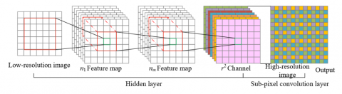
Figure 1. Sub-pixel convolution processing procedure
At the same time, the design principle of sub-pixel convolution optimizes the upsampling process by using the PixelShuffle layer, greatly improving the upsampling efficiency. In the task of cropland non-grain transformation identification in China, the spatial scale of land object changes is often small, and the boundaries of cropland and the details of land use changes are often hidden in complex terrain and backgrounds. After applying the PixelShuffle layer, the pixels in the feature map are rearranged so that the number of rows and columns is expanded to the target multiple, while maintaining the integrity of the features. This process can effectively enlarge the size of the feature map without causing information loss or unnecessary blurring. Figure 1 shows the sub-pixel convolution processing procedure.
In the task of identifying the spatial differentiation of cropland non-grain transformation, land object changes may exhibit complex and nonlinear features, and traditional linear processing methods often cannot effectively extract these complex features. Therefore, the upsampling module introduces multiple convolutional layers and ReLU activation functions in each module to enhance the network's nonlinearity and learning ability. By using convolutional layers to extract features in the upsampling module, increasing the number of channels of the feature maps, and using ReLU activation functions to enhance the nonlinear characteristics of the network, the model can better handle complex cropland changes. This design helps the model better adapt to different geographical and environmental backgrounds when processing various cropland non-grain transformation features in different regions of China, thereby improving the identification accuracy and robustness.
2.3 Classifier
In the task of identifying the spatial distribution of cropland non-grain transformation, each pixel represents a portion of geographic information in remote sensing imagery, and these pixels may encompass various land use types. Utilizing the Softmax function, the model's classifier maps each pixel's output to probability values across multiple categories, such as cropland, non-grain cropland, urban construction land, etc. The application of the Softmax function ensures that the output results are in the form of a probability distribution, providing a clear probability value for each pixel's corresponding category, facilitating subsequent analysis and decision-making. The classifier also processes the feature maps from the upsampling module to accomplish specific pixel-level classification tasks. In the process of identifying cropland non-grain transformation, the spatial resolution and detail representation of remote sensing imagery are crucial. The optimized sub-pixel segmentation model extracts finer feature information and maps it to pixel-level classification, effectively distinguishing land types with subtle differences. The classifier's design employs the category probability vector generated by the Softmax function, determining the specific category of each pixel based on the maximum probability value. Specifically, for a training dataset composed of v labeled samples {(a(1),b(1))...(a(v), b(v))}, where the input is denoted by au and the output includes j types b(u)∈{0.1..j}, assuming the training model parameters are represented by ϕ, and the normalization of the probability distribution is given by 1/∑jm=1rSma(u), the probability of classifying au into category k can be calculated by the following formula:
$o\left(b^{(u)}=k \mid a^{(u)} ; \varphi\right)=\frac{r_k^S a^{(u)}}{\sum_{m=1^{s_m^m}}^j a^{(u)}}$ (3)
2.4 Model optimization
In the task of identifying cropland non-grain transformation, each pixel may belong to different categories, such as cropland, non-grain cropland, non-cropland, etc. The cross-entropy loss function quantifies classification accuracy by comparing the predicted category probability distribution with the actual category labels. Therefore, this study employs the minimization of cross-entropy loss, enabling the model to continuously adjust predictions during training, bringing each pixel's classification result closer to the true label, thereby enhancing identification accuracy, especially in complex boundary regions or transition zones. In practical application, assuming the transposed category label corresponding to a pixel is represented by $b_u^T$, the number of pixels in a single image is denoted by L, and the predicted probability output by the sub-pixel segmentation model is ou, the calculation formula for the cross-entropy loss function is:
$M_{Z R}=-\frac{1}{L} \sum_{u=1}^L\left(b_u^T \log \left(o_u\right)\right)$ (4)
Overfitting may lead the model to perform well on the training set but poorly in actual applications, particularly when handling unseen regions or remote sensing data from different years, resulting in reduced generalization capability and decreased identification accuracy. To effectively address this issue, L2 regularization is introduced into the loss function to reduce the model's over-reliance on certain features during training. By incorporating the L2 norm of the network weight matrix into the loss function, the regularization term suppresses excessive weights, encouraging the network to learn smaller and more dispersed weights. For the task of identifying the spatial distribution of cropland non-grain transformation, this approach helps the model avoid overfitting specific detail features, thereby enhancing the model's adaptability across various environments and geographic backgrounds. Let the original cross-entropy loss function be denoted by C0, the regularization coefficient by η, and the L2 regularization term by η/2vΣqq2, then the calculation formula for the loss function after regularization is:
$C=C_0+\frac{\eta}{2 v} \sum_q q^2$ (5)
In the application scenario of identifying the spatial distribution of cropland non-grain transformation, remote sensing imagery typically involves large-scale geographic data, including changes across different years, regions, and land use types. Batch normalization aids the model in better handling these complex spatial features, particularly for different patterns and heterogeneous features in large-scale datasets. Batch normalization effectively ensures data consistency across different batches, avoiding performance fluctuations caused by statistical differences between data batches. Assuming the input data of the j-th layer is represented by a(j), and the mean and variance of the j-th layer are denoted by ω(j), a(j) is used to avoid zero-error, with ε(j) and α(j) being learnable parameters. The calculation formulas for the mean and variance within a batch are:
$\begin{aligned} & \hat{a}^{(j)}=\frac{a^{(j)}-\omega^{(j)}}{\sqrt{\delta^{2(j)}+\epsilon}} \\ & b(j)=\varepsilon^{(j)} \hat{a}^{(j)}+\alpha^{(j)}\end{aligned}$ (6)
In order to deeply understand the long-term trend, spatial expansion, and potential impact of the non-grain transformation of cropland, after identifying the spatial distribution differentiation of non-grain transformation of cropland in China, this paper further conducts an analysis of the spatial dynamic evolution of cropland non-grain transformation in China. Specifically, the first step is to monitor and analyze the non-grain transformation areas of cropland regularly through multi-temporal remote sensing data. By comparing remote sensing images of multiple time periods, it is possible to reveal the spatial distribution patterns of cropland transformation to non-grain use at different time points. In this process, the model first analyzes the changes in cropland at each time node, identifies the areas where cropland has undergone non-grain transformation, and tracks the expansion or contraction of the non-grain transformation phenomenon through a multi-temporal differentiation identification method. Using time series data, the speed, scale, and change trends of cropland non-grain transformation can be quantitatively evaluated from both spatial and temporal dimensions.
Dynamic evolution analysis can be conducted more deeply through land use change models. These models can fit and predict the historical data of the spatial distribution of cropland non-grain transformation to identify possible change trends and future evolution directions of non-grain transformation areas. For example, based on the optimized sub-pixel segmentation model that identifies non-grain transformation areas, the relationship between these areas and factors such as land use, policy adjustment, and market demand can be further analyzed. Regression analysis or machine learning models can be used to evaluate the influence of different factors on the non-grain transformation of cropland. Combined with prediction models, the possible evolution paths of cropland non-grain transformation under different scenarios can be inferred.
Further analysis also needs to combine the dynamic evolution of non-grain transformation with the actual grain production capacity for comprehensive evaluation. The non-grain transformation of cropland is not only a change in land use patterns, but also directly affects the stability and security of grain production. Therefore, when studying the dynamic evolution of cropland non-grain transformation, it is necessary to combine it with the grain production potential of the region to analyze the degree of weakening of grain production capacity in non-grain transformation areas. This process requires retrospective analysis of historical data of grain production in each region and also needs to consider the potential impact of future policy adjustments on grain production capacity. For example, the cropland in some high-efficiency agricultural areas or major grain-producing areas may be converted to high-value crop or construction land, which may lead to a significant decline in grain production capacity. However, in some relatively remote areas, the non-grain transformation phenomenon may not have a major impact on the overall grain supply. Therefore, by analyzing the relationship between the spatial differentiation of non-grain transformation and the grain production potential in each region, it is possible to better assess the actual threat of “non-grain transformation” to grain production security.
The spatial differentiation of cropland “non-grain transformation” is not only related to economic development and policy decision-making, but also has a profound impact on the stability and security of grain production in China. With the rapid development of China’s economy and the advancement of urbanization, some cropland has been transferred to industrial, urban construction, and ecological protection uses, resulting in a reduction of grain production area. In particular, some farmland has been converted to high-value crop cultivation or industrial use. This kind of land use non-grain transformation directly affects the supply and self-sufficiency capacity of grain. Through dynamic evolution analysis of the spatial distribution of “non-grain transformation” in various regions of China, it is possible to identify the most high-risk areas, such as regions where large areas of cropland are converted to non-grain crops or urban construction land. The grain production potential in these areas decreases year by year and may even lead to grain supply shortages. Especially in China’s main grain-producing areas, if the process of “non-grain transformation” is too fast, it may pose a threat to overall food security. Therefore, through dynamic evolution analysis, it is not only possible to visually understand the distribution changes of cropland non-grain transformation, but also to help the government and decision-makers formulate more precise land management and food security protection policies at the regional level to ensure national food security.
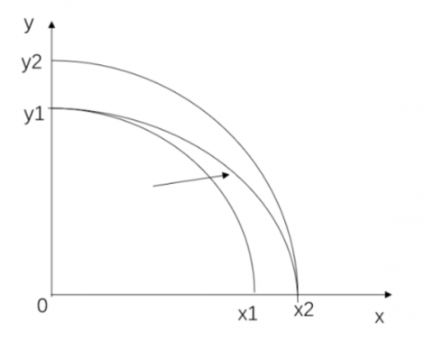
Specifically, assuming that domestic and international institutional policies remain stable and current technologies do not change, this paper only analyzes the impact of the cropland “non-grain transformation” on grain production caused by changes in the planting structure of cropland. X and Y represent grain yield and the output obtained from non-grain transformation of cropland, respectively. A represents the original land production combination point. If farmers choose to plant non-grain crops, the corresponding grain output will be reduced, so the Y output will not change in the short term, while the X output will decrease. An implicit condition in the production possibility curve is that any economic behavior must make a choice. For example, if grain is chosen to be planted, then planting non-grain crops cannot be chosen.
Under the condition that the cropland area remains unchanged, the production combination point on the production possibility curve moves from point A to point B (see Figure 2). At this time, the production combination point is B (x2, y2). From the point on Y1X1 above, the utility brought to farmers is the same. From the perspective of marketization, the non-grain transformation of cropland has, to a certain extent, realized the reallocation of resources. The re-combination of land factors may be optimized. However, in the actual process of economic development, these non-grain transformation uses will cause the cropland area to continuously decrease, thereby leading to a reduction in the total amount of cropland used for grain production. The production possibility curve moves from Y2X2 to Y1X1, and the production combination point drops from point B to point B'. Moreover, all utility values on X1Y1 are lower than the utility values on curve X2Y2, resulting in a decrease in resource allocation efficiency. From this change process, it can be seen that the decrease in cropland area leads to a reduction in the total output of cropland, and the total grain output will naturally decrease, thereby threatening food security.
Figure 2. Production possibility curve under price changes and cropland area changes
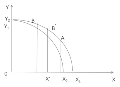
When agricultural production technology in grain production and production technology in non-grain transformation of cropland are both improved, the production possibility curve moves along the direction of the arrow in Figure 3. The production possibility curve moves from Y1X1 to Y1X2, which will lead to an increase in the total output of cropland under the condition that the cropland remains unchanged. When the production technology in grain production improves while the speed of cropland non-grain transformation remains unchanged, the grain output of cropland will increase, while the non-grain transformation output will remain unchanged.
Figure 3. Production possibility curve under technological changes
4.1 Variable selection and data sources
This study takes the panel data of the proportion of cropland "non-grain transformation" area from 2005 to 2020 in 31 provinces across the country (excluding Hong Kong, Macao, and Taiwan) as the research object. Drawing on previous research results, this paper explores the relationship between variables based on the spatial econometric model and analyzes the impact of cropland non-grain transformation on grain production under spatial conditions. The dependent variable selected to represent grain production is the total grain output; the core explanatory variable is the proportion of cropland "non-grain transformation" area, represented by the ratio of non-grain transformation cropland area to the total sown area of crops. The non-grain transformation area is calculated as the difference between the sown area of all crops and that of grain crops. Control variables include rural employment, fertilizer usage, total agricultural machinery power, per capita GDP, Engel coefficient of rural households, total agricultural output value, and the proportion of farmland transfer. The data are sourced from the National Rural Contract Management Status, China Statistical Yearbook, and China Rural Statistical Yearbook, etc.
4.2 Descriptive statistics
As shown in Table 1, grain output (Y) refers to the total quantity of grain produced in a year, with the minimum value being 883,000 tons in Qinghai Province in 2006, and the maximum value being 75.06 million tons in Heilongjiang Province in 2020; rural employment (JS) is replaced by data on agriculture, forestry, animal husbandry, and fishery from regional statistical yearbooks, with the minimum being 453,100 persons in Shanghai in 2005 and the maximum being 31.3883 million persons in Henan in 2020; fertilizer usage (H1) has a mean of 1.8126 million tons; the minimum usage of agricultural machinery power (H2) is 94 in Shanghai in 2020; cropland non-grain transformation rate (GD) is expressed as the ratio of non-grain transformation cropland area to sown crop area, with a national average of 35% from 2005 to 2020; per capita GDP (JX) ranges from a minimum of 8,009 yuan to a maximum of 97,300 yuan. Engel coefficient of rural residents (Rec) is expressed as a percentage, measured by the proportion of household consumption expenditure to total expenditure, with an average of about 38%; total agricultural output value (Tva) refers to the total value of agricultural production in a year, with an average of 141 billion yuan from 2005 to 2020; the farmland transfer ratio (Trans) is expressed as the ratio of farmland transfer area to cropland area, with the national farmland transfer proportion being about 30% in 2020.
Table 1. Descriptive statistics of variables
|
Variable Name |
Variable Description |
Mean |
Std. Dev. |
Min |
Max |
|
Y |
Total grain production in a year (10,000 tons) |
1847.02 |
1556.50 |
88.3 |
7506.80 |
|
GD |
Ratio of non-grain transformation cropland area to crop sown area (%) |
0.35 |
0.13 |
0.04 |
0.67 |
|
JS |
People aged 16 and above in rural areas engaged in production (agriculture, forestry, animal husbandry, fishery) (10,000 persons) |
1382 |
1427 |
45.31 |
3138.83 |
|
H1 |
Fertilizer usage amount (10,000 tons) |
181.26 |
145.10 |
4.21 |
716.10 |
|
H2 |
Total rated power of agricultural machinery |
3046.75 |
2839.77 |
94 |
13353 |
|
JX |
Indicator measuring economic development level (yuan) |
17315.29 |
16496.34 |
8009 |
97277.77 |
|
REC |
Engel coefficient of rural households (%) |
38 |
23.81 |
57.63 |
7.14 |
|
TVA |
Total agricultural output value (100 million yuan) |
1410 |
36.41 |
4973 |
1123 |
|
Trans |
Ratio of farmland transfer area to cropland area |
0.21 |
0.01 |
0.87 |
0.17 |
4.3 Spatial analysis of China's cropland conversion
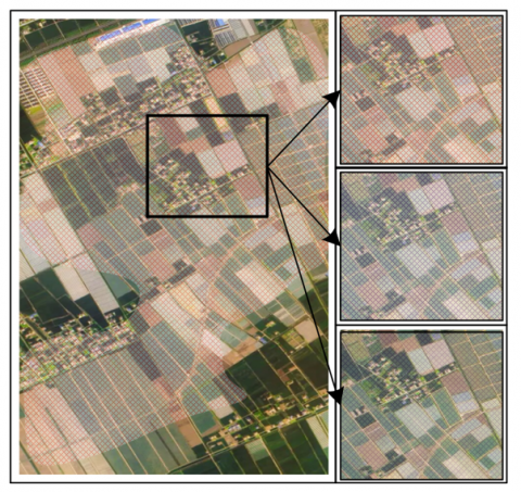
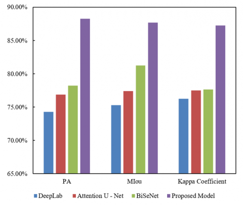
Figure 4 shows the high-precision spatial differentiation recognition effect diagram of medium-resolution cropland remote sensing images. Furthermore, this paper conducts a comparative study on the proposed method. According to the results of evaluation metrics comparison in Figure 5 and Table 2, it can be clearly seen that the proposed model in this paper outperforms other models in accuracy. Specifically, in the three evaluation metrics—Pixel Accuracy (PA), Mean Intersection over Union (MIou), and Kappa Coefficient—the proposed model achieves 88.26%, 87.69%, and 87.26% respectively. In contrast, the PA, MIou, and Kappa coefficients of DeepLab, Attention U-Net, and BiSeNet are all lower than those of the proposed model, which are 74.26%, 75.26%, 76.23%, 76.85%, 77.41%, 77.51%, 78.21%, 81.26%, and 77.63%, respectively. The data show that the proposed model exceeds all other comparison models in all three evaluation metrics, especially in PA and MIou, indicating that the proposed model has higher recognition accuracy in the task of spatial differentiation recognition of cropland non-grain transformation. From the data analysis in Table 2, it can be seen that the optimized sub-pixel segmentation model proposed in this paper performs significantly better than other common models in the task of spatial differentiation recognition of cropland non-grain transformation, indicating that it has higher accuracy and stability. In particular, the proposed model outperforms BiSeNet by 10.05% and 6.43% in PA and MIou respectively, showing its significant advantages in spatial distribution accuracy and category segmentation accuracy. The improvement of the Kappa coefficient further verifies the superiority of the proposed model in classification consistency, indicating that the model not only performs better in overall accuracy but also effectively reduces classification bias.
Table 2. Comparison of evaluation metrics for different models
|
|
PA |
MIou |
Kappa Coefficient |
|
DeepLab |
74.26% |
75.26% |
76.23% |
|
Attention U - Net |
76.85% |
77.41% |
77.51% |
|
BiSeNet |
78.21% |
81.26% |
77.63% |
|
Proposed Model |
88.26% |
87.69% |
87.26% |
Figure 4. High-precision spatial differentiation recognition effect diagram of medium-resolution cropland remote sensing images
Figure 5. Comparison of evaluation metrics for different models
Figure 6. Comparison of extraction accuracy indicators before and after model optimization
Table 3. Comparison of extraction accuracy indicators before and after model optimization
|
|
PA |
MIou |
Kappa Coefficient |
|
Before optimization |
91.26% |
91.47% |
89.62% |
|
After optimization |
88.31% |
89.32% |
87.26% |
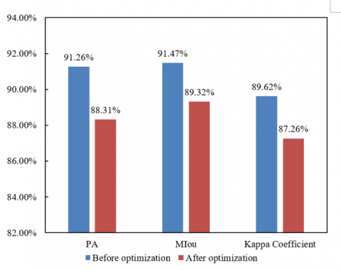
According to the comparison results of extraction accuracy indicators before and after model optimization in Figure 6 and Table 3, it can be seen that the model before optimization is superior to the optimized model in PA, MIou, and Kappa coefficient. Specifically, the PA before optimization is 91.26%, the MIou is 91.47%, and the Kappa coefficient is 89.62%; while the optimized model is 88.31%, 89.32%, and 87.26% respectively. These data show that although the optimized model has slightly decreased in all indicators, the model before optimization performs better in terms of accuracy. Especially, the PA and MIou decreased significantly by 2.95% and 2.15% respectively, and the Kappa coefficient also decreased by 2.36%. This result indicates that although optimization may introduce some loss of accuracy, the optimized model may have improved its efficiency or processing capacity in other aspects, which is worth further exploration. From the data analysis in Table 3, the differences in accuracy indicators before and after optimization suggest that the optimization process may have sacrificed part of the accuracy in exchange for higher computational efficiency or better adaptability. The superior performance of the model before optimization in PA, MIou, and Kappa coefficient indicates its high accuracy in identifying the spatial differentiation of cropland non-grain transformation, and it can more accurately identify different types of non-grain areas. However, although the optimized model has declined in accuracy, it still maintains relatively stable performance, indicating that the optimization process may have had a positive impact on improving the model's computing efficiency, model stability, or generalization ability.
4.4 Spatial econometric model setting
The first law of geography states that "everything is related to everything else, but near things are more related than distant things". Applying this to spatial locations is also applicable, that is, there is extensive connection between regions within a spatial range. Therefore, studying the trend of cropland non-grain transformation from a spatial perspective helps to more comprehensively understand the situation of cropland planting. To make the conclusion more credible, this paper uses the spatial geographical weight matrix Wij in spatial analysis to construct the spatial weight matrix. Specifically, Wij=1/dij, where dij refers to the geographical distance (the adjacent distance between regions), and the element Wij in W defines the spatial adjacency relationship, where adjacent is 1 and otherwise 0, forming a 0-1 matrix. Specifically, the spatial econometric regression model is constructed as follows:
$\begin{aligned} \ln Y_{i, t} & =\alpha_0+\alpha_1 G D_{i, t}+\alpha_2 J S_{i, t} \\ & +\alpha_3 J X_{i, t}+\alpha_4 H_{i, t}+\alpha_5 \text { trans }_{i, t} \\ & +\alpha_6 T V A+\alpha_7 R E C_{i, t}+\varepsilon_{i, t}\end{aligned}$ (7)
In the equation, Y represents total grain output, GD represents non-grain rate, JS represents rural employees, JX represents per capita GDP, Tva represents total agricultural output value, H includes variables such as fertilizer usage amount (H1) and total agricultural machinery power (H2), rec represents the Engel coefficient (%) of rural resident households in China, and trans represents the proportion of farmland transfer (%). α0 is the constant term, and ε represents the random error term.
Using the spatial analysis functions of GeoDa, ArcGIS 10.6, and Stata software, this paper explores the spatial distribution patterns and characteristics of cropland non-grain transformation. When using spatial models to analyze data, it is first necessary to test the spatial autocorrelation, which includes local and global types. "Moran’s I" is currently the commonly used method for calculating global spatial autocorrelation. Moran’s I is the earliest method for measuring spatial autocorrelation. The main idea of this method is to study the distribution of two or more units in space. The calculation formula is:
$\begin{aligned} & I=\frac{\sum_{i=1}^n \sum_{j=1}^n w_{i j}\left(x_i-\bar{x}\right)\left(x_j-\bar{x}\right)}{S^2 \sum_{i=1}^n \sum_{j=1}^n w_{i j}} \\ & S^2=\sum_{i=1}^n \frac{\left(x_i-\bar{x}\right)^2}{n}\end{aligned}$ (8)
where, S2 is the sample variance, Wij is the spatial weight matrix, and the elements i and j represent the spatial distance between region i and region j, the smaller Wij, the larger the interval value. The value range of Moran’s I is between -1 and 1. A value greater than 0 indicates positive autocorrelation, that is, high values and high values or low values and low values exist in neighboring units. Conversely, a value less than 0 indicates negative autocorrelation, i.e., high and low values exist in neighboring units. It can be understood as: First, a high-high agglomeration area formed by non-grain rates, indicating high non-grain rates and small differences with neighboring regions. Second, a high-low agglomeration area is formed, indicating large differences in non-grain rates with neighboring regions. Third, a low-low agglomeration area is formed, where non-grain rates are low and differences with adjacent units are small. Using GeoDa software to measure the spatial agglomeration characteristics of “non-grain transformation” from 2009 to 2020, the results are consistent with existing research conclusions. As shown in Figure 7, the results of global Moran’s I for non-grain rate are: 0.343, 0.365, 0.303, 0.369, 0.451, 0.410, 0.409, 0.439, 0.484, 0.512, 0.537, and 0.507. The results of Moran’s I are positively significant, which also means that regions with high values and high values or low values and low values have small differences in adjacent areas, appearing in the first and third quadrants. In reality, this indicates that provinces with similar geographical attributes are clustered in space. Stata calculates a P-value of 0.021, indicating that for the hypothesis of non-grain rate autocorrelation, the null hypothesis of "no spatial autocorrelation" is rejected, that is, spatial correlation exists.
Figure 7. Global Moran’s I of national non-grain rate from 2009 to 2020
4.5 Spatial panel model regression analysis
The Hausman test can determine whether to choose fixed effects or random effects. The result of the Hausman test shows that the p-value approaches 0, indicating that the null hypothesis of random effects is rejected at the 1% significance level. Therefore, the fixed effects model is selected. Since the Moran index indicates that the proportion of non-grain cropland has spatial correlation, and to reasonably expect results, this paper uses the lag term of food security in the spatial Durbin model to deal with endogeneity issues. The regression results obtained through model calculation are shown in Table 4.
Table 4. Regression result analysis of the spatial model
|
Variable |
Standard Error |
Coefficient |
P-Value |
|
L.GD Non-grain Cropland Rate (%) |
0.21 |
-0.15** |
0.008 |
|
H2 Total Agricultural Machinery Power |
0.13 |
0.73** |
0.003 |
|
H1 Fertilizer Use (10,000 tons) |
0.33 |
-0.54** |
0.021 |
|
JS Rural Employees (10,000 persons) |
0.15 |
0.61** |
0.010 |
|
Trans Agricultural Land Transfer Rate (%) |
0.84 |
0.42** |
0.024 |
|
TVA Gross Agricultural Output Value (100 million yuan) |
0.63 |
0.68** |
0.018 |
|
JX Per Capita GDP (yuan) |
0.18 |
0.19** |
0.011 |
|
REC Engel Coefficient of Rural Households (%) |
0.38 |
0.06** |
0.032 |
|
Constant (con) |
0.17 |
-0.56** |
0.017 |
Note: * indicates significance at the 0.1 level, ** at the 0.05 level, and *** at the 0.001 level.
Based on the constructed spatial regression model under the assumption conditions, the coefficient of non-grain transformation cropland rate is -0.15, indicating that the non-grain transformation rate is negatively correlated with food security. This means that a reduction in grain planting area will threaten food security in China. According to the data, if the non-grain transformation rate increases by 1%, the grain production output will decrease by 0.15%. However, in reality, improvements in production technology can compensate for the losses caused by the non-grain transformation of cropland. On one hand, with a small reduction in cropland area and under unchanged grain yield per unit area, reducing grain sowing area will inevitably lead to a decrease in total grain output. On the other hand, the expansion of non-grain planting area will also pose a threat to grain output, which will endanger the supply of basic food and thus threaten China's food security. The higher the amount of fertilizer used, the more unfavorable it is for the sustainable development of land. A larger grain sowing area is, paradoxically, not conducive to food security. Currently, the area is 11.67 × 10⁷ hectares. Although there is some room for reduction, land use should be scientifically based, and the non-grain transformation phenomenon should be viewed dialectically. If grain sowing area is excessively reduced, under the same production conditions, encountering severe natural disasters such as cold dew wind and low temperature with overcast rain in the short term will lead to a tight domestic grain supply, and food security cannot be guaranteed. The conclusions of the study are as follows: First, the crop planting structure is unreasonable. The grain production structure should be adjusted reasonably according to the upgraded food consumption needs of residents to provide rich and high-quality grain products. Second, the imbalance between grain supply and demand to some extent indicates that the country’s effective grain supply is insufficient to meet the real demand of residents.
According to regional differences, to better illustrate the spatial differences in non-grain transformation of cropland, the 31 provinces in China are divided into four regions according to the classification of the statistical yearbook: Northeast (Heilongjiang, Jilin, and Liaoning), Central (Shanxi, Anhui, Jiangxi, Henan, Hunan, and Hubei), Western (Inner Mongolia, Guangxi, Chongqing, Sichuan, Guizhou, Yunnan, Tibet, Shaanxi, Gansu, Qinghai, Ningxia, and Xinjiang), and Eastern (Beijing, Tianjin, Hebei, Shanghai, Jiangsu, Zhejiang, Fujian, Shandong, Guangdong, and Hainan).
Table 5. Spatial model regression result analysis among different regions
|
Variable |
Robust Standard Error |
Coefficient |
P-Value |
|
Eastern Region |
0.31 |
-0.649** |
0.035 |
|
Central Region |
1.05 |
-0.509* |
0.063 |
|
Western Region |
0.86 |
-2.066** |
0.016 |
|
Northeast Region |
0.28 |
-2.682*** |
0.000 |
As shown in Table 5, the result shows that the coefficient value is the highest in the Northeast region, which indirectly indicates that the impact of non-grain transformation in the main grain-producing areas on food security is greater than in non-main grain-producing areas. This confirms that the non-grain rate of cropland spreads spatially and the influence of non-grain transformation in main production areas is greater than in general areas, providing theoretical and practical basis for the government to curb non-grain transformation behavior. In all four regions, the non-grain transformation of cropland has a negative impact on food security. The coefficient of non-grain cropland rate in the Northeast region has the greatest impact on food security, followed by the Western region. The possible reason is that the Western region has poor resource conditions and the least amount of cropland. Compared with other regions, the non-grain transformation rate is not high. Farmers in the West still grow staple food crops on their limited land. Therefore, the level of non-grain transformation is lower than that in the Central and Eastern regions and is second only to the Northeast region. Again, the non-grain transformation rate of cropland in the Central and Eastern regions ranks lower among the four regions. Their impact coefficients on food security are lower than in the Northeast, which is a reasonable situation. Overall, the non-grain transformation rate in all 31 provinces (municipalities) has a negative impact on food security. This also reminds us to promptly curb non-grain transformation behavior to ensure that the area of grain cultivation does not decrease, stabilize grain production, and achieve the goal of food security.
This paper accurately identified the spatial distribution characteristics of China's non-grain cropland through the optimized sub-pixel segmentation model and proposed a dynamic evolution analysis framework for non-grain transformation. The first part of the study mainly relied on the optimized sub-pixel segmentation model to accurately identify the spatial distribution of non-grain cropland in China. Compared with DeepLab, Attention U-Net, and BiSeNet models, the model in this paper showed significant advantages in key evaluation metrics such as PA, MIou, and Kappa coefficient, especially in the accurate identification of spatial non-grain cropland. The second part of the study constructed a dynamic evolution analysis framework for non-grain cropland, aiming to reveal the evolution pattern of non-grain transformation in different regions and time scales. By comparing multi-temporal remote sensing data, the spatiotemporal variation trend of non-grain transformation was analyzed. Combined with land use change models, the relationship between non-grain transformation and policies, market demand, and other factors was explored, providing scientific evidence for policy-making and land management.
The important value of this research lies in proposing an optimized sub-pixel segmentation model that can accurately identify the spatial distribution characteristics of non-grain cropland, and combining it with a dynamic evolution analysis framework to provide a new research perspective for deeply understanding the change pattern of non-grain transformation. This work not only improved the accuracy of non-grain cropland identification but also provides scientific evidence for cropland protection and sustainable agricultural development. At the policy level, the study provided quantitative support for land resource management and cropland protection measures.
The limitations of the study mainly lie in the fact that although the model improves identification accuracy, there is still some uncertainty and error in the identification of non-grain transformation in certain areas, which may be related to the resolution of remote sensing data, terrain complexity, and model parameter settings. In addition, this study mainly relies on remote sensing images for analysis, and may not fully take into account the dynamic impact of other socio-economic factors, which to some extent limits the comprehensiveness and accuracy of the analysis.
Future research can further optimize the sub-pixel segmentation model by integrating multi-source data to improve the generalization and accuracy of the model. In terms of dynamic evolution analysis, more advanced time-series analysis methods, such as time series models in deep learning, can be introduced to further improve the prediction ability of non-grain transformation trends. Future research should also enhance the cross-regional adaptability of the model, especially in validation across different geographic environments, to ensure the universality and reliability of the research results nationwide. Finally, considering the close relationship between non-grain transformation of cropland and food security, ecological environment, etc., future research can expand this into broader land use change and sustainable development research, providing stronger decision-making support for food security and environmental protection under global change.
[1] Kutyauripo, I., Mavodza, N.P., Gadzirayi, C.T. (2021). Media coverage on food security and climate-smart agriculture: A case study of newspapers in Zimbabwe. Cogent Food & Agriculture, 7(1): 1927561. https://doi.org/10.1080/23311932.2021.1927561
[2] Zurba, M., Islam, D., Smith, D., Thompson, S. (2012). Food and healing: An urban community food security assessment for the north end of Winnipeg. Urban Research & Practice, 5(2): 284-289. https://doi.org/10.1080/17535069.2012.691624
[3] Ismail, N.H., Zulfa, N.Q.A., Ramly, A.S.M., Sharif, M.S.M., Nor, N.M. (2024). The food insecurity issues in gastronomy tourism among local and international tourists in Malaysia. Jurnal Gizi dan Pangan, 19(1): 105-110. https://doi.org/10.25182/jgp.2024.19.Supp.1.105-110
[4] Ran, R., Hua, L., Li, T., Chen, Y., Xiao, J. (2023). Why have China’s poverty eradication policy resulted in the decline of arable land in poverty-stricken areas? Land, 12(10): 1856. https://doi.org/10.3390/land12101856
[5] Yin, G., Lou, Y., Xie, S., Wei, W. (2022). Evaluation of the response of grain productivity to different arable land allocation intensities in the land use planning system of China. Sustainability, 14(5): 3109. https://doi.org/10.3390/su14053109
[6] Ye, S., Song, C., Gao, P., Liu, C., Cheng, C. (2022). Visualizing clustering characteristics of multidimensional arable land quality indexes at the county level in mainland China. Environment and Planning A: Economy and Space, 54(2): 222-225. https://doi.org/10.1177/0308518X211062232
[7] Li, X., Shen, L., Wang, H.S. (2019). The follow rotation implementation of arable land and the impact of agricultural production in China. Fresenius Environmental Bulletin, 28(12A): 10247-10255. https://doi.org/10.5555/20219911403
[8] Ma, L., Pan, Z., Wang, Y., Wei, F. (2022). Spatial distribution characteristics and influencing factors of the success or failure of China’s overseas arable land investment projects—based on the countries along the “belt and road”. Land, 11(11): 2090. https://doi.org/10.3390/land11112090
[9] Min, M., Miao, C., Duan, X., Yan, W. (2022). Formation mechanisms and general characteristics of cultivated land use patterns in the Chaohu Lake Basin, China. Land Use Policy, 117: 106093. https://doi.org/10.1016/j.landusepol.2022.106093
[10] Wu, Z., Fan, Q., Li, W., Zhou, Y. (2024). The spatial–temporal evolution and impact mechanism of cultivated land use in the mountainous areas of southwest Hubei province, China. Land, 13(11): 1946. https://doi.org/10.3390/land13111946
[11] Deng, X., Huang, J., Rozelle, S., Zhang, J., Li, Z. (2015). Impact of urbanization on cultivated land changes in China. Land Use Policy, 45: 1-7. https://doi.org/10.1016/j.landusepol.2015.01.007
[12] Arowolo, A.O., Deng, X. (2018). Land use/land cover change and statistical modelling of cultivated land change drivers in Nigeria. Regional Environmental Change, 18: 247-259. https://doi.org/10.1007/s10113-017-1186-5
[13] Lan, Y., Xu, B., Huan, Y., Guo, J., Liu, X., Han, J., Li, K. (2023). Food security and land use under sustainable development goals: Insights from food supply to demand side and limited arable land in China. Foods, 12(22): 4168. https://doi.org/10.3390/foods12224168
[14] Ye, S., Song, C., Shen, S., Gao, P., Cheng, C., Cheng, F., Zhu, D. (2020). Spatial pattern of arable land-use intensity in China. Land Use Policy, 99: 104845. https://doi.org/10.1016/j.landusepol.2020.104845
[15] Ai-Mashagbah, A.F., Ibrahim, M. (2021). Integration of remote sensing and GIS to detect the spatial and temporal changes of land use and land cover in Jerash governorate, North-West Jordan. Fresenius Environmental Bulletin, 30(8): 9788-9794.
[16] Habte, D.G., Belliethathan, S., Ayenew, T. (2021). Evaluation of the status of land use/land cover change using remote sensing and GIS in Jewha Watershed, Northeastern Ethiopia. SN Applied Sciences, 3(4): 501. https://doi.org/10.1007/s42452-021-04498-4
[17] Peng, B., Li, Y., Elahi, E., Wei, G. (2019). Dynamic evolution of ecological carrying capacity based on the ecological footprint theory: A case study of Jiangsu province. Ecological Indicators, 99: 19-26. https://doi.org/10.1016/j.ecolind.2018.12.009