Nuo Li![]() | Qiang Miao*
| Qiang Miao*![]()
© 2025 The authors. This article is published by IIETA and is licensed under the CC BY 4.0 license (http://creativecommons.org/licenses/by/4.0/).
OPEN ACCESS
To address altitude estimation inaccuracies in Unmanned Aerial Vehicles (UAVs) under non-Gaussian noise and intermittent sensor failures, this paper proposes a Long Short-Term Memory (LSTM)-Kalman cooperative architecture that establishes symbiotic interaction between deep feature extraction and physical filtering. The core innovation lies in bidirectional cyclic learning: LSTM layers distill temporal noise patterns while Kalman modules inject state-space constraints through differentiable projection. A manifold interpolation mechanism resolves multi-rate signal mismatches, utilizing LSTM-derived coherence weights to guide Lie group synchronization for phase distortion suppression. The framework incorporates a fractal-aware decoupling network where LSTM cells generate adaptive masks, dynamically separating Gaussian/non-Gaussian components to reconstruct Kalman gain rules. Experimental validation demonstrates the architecture's superiority in balancing physical consistency and learning capability, providing a novel paradigm for robust navigation signal fusion under complex noise conditions.
Long Short-Term Memory (LSTM)-Kalman symbiotic architecture, non-Gaussian noise suppression, manifold interpolation synchronization, embedded real-time fusion
The reliable operation of UAVs in complex environments, such as executing obstacle avoidance in urban areas or stabilizing attitude during disaster response operations, places stringent demands on the accurate prediction of their altitude information. Precise altitude prediction is a critical factor in ensuring mission success and flight safety. However, achieving high-accuracy, high-robustness altitude prediction in practical applications faces numerous challenges, particularly at low altitudes or in signal-degraded environments. Traditional physics-based modeling approaches, such as Kalman filtering [1], provide a rigorous framework for state estimation but often exhibit performance degradation when confronted with non-Gaussian noise distributions induced by factors like low-altitude turbulence [2], or spatiotemporal mismatches caused by effects such as multipath [3]. These phenomena lead to systematic deviations between theoretical models and actual dynamic characteristics, potentially compromising altitude estimation accuracy during critical operations.
In recent years, deep learning techniques have offered new avenues for addressing complex problems in sensor data processing. For instance, spatiotemporal convolutional networks enhance nonlinear modeling capabilities through multi-level feature extraction [4], while improved LSTM architectures demonstrate significant advantages in temporal dependency modeling. Nevertheless, existing purely data-driven methods still exhibit limitations when applied to UAV altitude prediction. On one hand, the "black-box" nature of network structures may overlook sensor physical constraints, posing risks of violating kinematic principles [5]. On the other hand, end-to-end training paradigms can disrupt causal relationships within signal processing chains, exacerbating spectral distortions in dynamic environments [6]. These issues are particularly pronounced in UAV altitude prediction tasks, which demand simultaneous adherence to physical consistency constraints and environmental adaptability.
To leverage the complementary strengths of model-driven and data-driven approaches, researchers have proposed various hybrid architectures. Among these, differentiable Kalman filtering frameworks optimize noise parameters via gradient propagation [7], while physics-embedded neural networks encode sensor characteristics as network priors [5]. Although these hybrid methods have achieved certain progress, several key challenges remain in enhancing UAV altitude prediction performance, such as effectively handling non-Gaussian noise and sensor spatiotemporal mismatches in complex environments, and improving the model's adaptive capability while ensuring physical consistency.
Addressing the aforementioned challenges, this study focuses on enhancing the accuracy and robustness of UAV altitude prediction in non-Gaussian environments. It proposes a novel LSTM-Kalman collaborative optimization architecture designed to deeply integrate physical constraints with data-driven optimization. The main contribution of this paper lies in constructing a fusion framework capable of effectively addressing sensor spatiotemporal mismatches and complex noise interference, thereby achieving more precise and reliable altitude state estimation. Theoretical analysis and experimental validation demonstrate that the proposed architecture effectively balances physical interpretability and environmental adaptability, offering a new technical pathway for improving the reliability of UAV navigation systems, particularly the altitude prediction subsystem.
The remainder of this paper is organized as follows: Section 2 reviews advancements and challenges in hybrid fusion architectures. Section 3 elaborates on the design principles and algorithmic implementation of the proposed collaborative optimization framework. Section 4 validates the method’s effectiveness through multidimensional experiments. Section 5 concludes the study and outlines future research directions.
2.1 Theoretical evolution of fusion paradigms
The theoretical development of sensor fusion technology has transitioned from model-driven to data-driven paradigms. Early research centered on the Kalman filtering framework, achieving state estimation through precise physical models, with these model-driven methods exhibit limitations in non-Gaussian scenarios due to rigid statistical assumptions [6]. Breakthroughs in deep learning have enabled data-driven paradigms to extract end-to-end features through spatiotemporal convolutional networks, significantly enhancing adaptability to complex environments [8]. The introduction of memory-augmented architectures further strengthens the system’s ability to model historical states, exhibiting robustness in scenarios with intermittent sensor failures [9]. However, purely data-driven approaches frequently suffer from kinematic distortion and energy non-conservation due to the lack of physical constraints, driving researchers to explore hybrid architectures.
2.2 Methodological breakthroughs in hybrid architectures
Current hybrid methodologies follow two technical paths: the first enhances traditional filters’ parameter adaptability through differentiable programming, such as differentiable Kalman frameworks that dynamically adjust noise covariance matrices via gradient propagation [10]; the second embeds physical conservation laws into neural network structures, exemplified by Hamiltonian dynamics-guided recurrent networks that preserve system energy properties through symplectic integration [11].
While such Hamiltonian-based approaches explicitly enforce specific conservation laws like energy through specialized network architectures, the LSTM-Kalman framework proposed in this work achieves physics-data synergy via a different mechanism. Our method focuses on establishing a deep, bidirectional coupling between the learned dynamics of the LSTM and the state-space constraints imposed by the Kalman filter structure. Physical consistency is thus maintained relative to the filter's model and enhanced through data-driven adaptation (e.g., via Bi-DGND and adaptive components), rather than through architectural enforcement of a specific conservation principle like energy.
While the former improves dynamic noise adaptation, it still depends on manually designed interpolation strategies for spatiotemporal alignment of multi-source heterogeneous sensors. The latter ensures physical consistency but is limited by the completeness of predefined constraints. Recent advancements have shifted focus toward co-designing sensor physical characteristics with computational frameworks, where joint hardware-algorithm optimization enables simultaneous noise suppression and temporal alignment through systematic integration of device-level features and algorithmic parameters [10, 11]. Nevertheless, existing methods exhibit delayed responses to sudden sensor degradation and unresolved geometric mismatches in cross-modal feature spaces.
2.3 New directions in physics-informed fusion learning
Physics-inspired machine learning provides novel theoretical tools for sensor fusion. Manifold-constrained learning frameworks significantly reduce Riemannian metric errors in multi-sensor data alignment by preserving the differential geometric properties of feature spaces [12]. The introduction of differentiable numerical simulators enables automatic satisfaction of mass-energy conservation laws during end-to-end training, offering a new paradigm for complex dynamic modeling. While these advancements improve fusion accuracy, theoretical gaps remain in designing online adaptation mechanisms for non-stationary environments, coupling sensor nonlinearities with algorithmic parameters, and developing lightweight deployment strategies for resource-constrained scenarios. This study addresses these challenges through a systematic solution: the LSTM-Kalman collaborative architecture achieves breakthroughs in manifold geometric modeling, dynamic noise decoupling, and hardware-algorithm co-optimization.
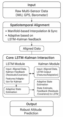
To address the challenge of inaccurate UAV altitude prediction under non-Gaussian noise, this paper proposes a novel architecture featuring deep collaboration between LSTM and a Kalman filter (the overall logic of which is illustrated in Figure 1). This method aligns multi-source sensor data using manifold geometry and leverages bidirectional information interaction between LSTM's data-driven analysis capabilities and the Kalman filter's physical model constraints. This achieves adaptive suppression of complex noise and precise modeling of system dynamics. Experimental results validate the effectiveness of this architecture in enhancing altitude prediction accuracy and robustness compared to traditional methods.
Figure 1. Flowchart of the LSTM-Kalman collaborative architecture
3.1 Generalized manifold interpolation compensation mechanism
3.1.1 $\mathrm{SE}(3) \times \mathbb{R}^4$ composite manifold construction
To fuse multi-source, heterogeneous sensor information (e.g., IMU, GPS, barometer with different sampling rates and noise characteristics) within a unified geometric framework for UAV systems, this paper proposes constructing a Lie group-based composite manifold. This manifold is designed to integrate the rigid-body motion state of the UAV with its spatiotemporal coordinates. We define this composite manifold space $\mathcal{M}$ as:
$\mathcal{M}=S O(3) \propto \mathbb{R}^3 \times \mathbb{R}^4$ (1)
where, $\mathrm{SE}(3)=\mathrm{SO}(3) \ltimes \mathbb{R}^3$ is the special Euclidean group, representing rotation (SO(3)) and translation $\left(\mathbb{R}^3\right)$ in 3D space. The additional $\mathbb{R}^4$ space encodes altitude (h), latitude $(\varphi)$, longitude $(\lambda)$, and time $(t)$.
To define distances and perform geometric operations on this manifold, we introduce a Riemannian metric tensor g. Considering the physical meaning of the subspaces and computational feasibility, we design g with a block-diagonal structure:
$g=\left(\begin{array}{lll}\omega_1 I_3 & 0 & 0 \\ 0 & \omega_2 I_3 & 0 \\ 0 & 0 & \omega_3 \operatorname{diag}\left(1, \cos ^2 \varphi, 1,1\right)\end{array}\right)$ (2)
Here, $I_3$ is the $3 \times 3$ identity matrix. This structure assumes that the metric contributions of rotation, translation, and the other state components are decoupled. The $\mathbb{R}^4$ component includes the $\cos ^2 \varphi$ term to properly handle the geometric properties associated with the geographic coordinate system (latitude $\varphi$, longitude $\lambda$). The scalar weights $\omega_1, \omega_2, \omega_3>0$ are used to adjust the relative scales of these subspaces within the manifold geometry. The choice of scalar weights, rather than full matrix blocks, primarily aims to simplify computations and parameter optimization, facilitating embedded implementation, while also intuitively reflecting the relative importance assigned to each subspace.
3.1.2 Adaptive metric weight optimization via LSTM-Kalman
A static manifold metric cannot adapt to dynamically changing sensor noise and operating environments. To enhance robustness, this paper introduces an adaptive metric weight optimization method based on an LSTM-Kalman collaborative mechanism. The weights $\omega_i$ are not fixed values but are dynamically adjusted based on real-time data.
This mechanism combines the strengths of data-driven and model-driven approaches:
Information from these two sources is fused via a mapping function $f(\cdot)$ to update the metric weights $\omega_i$ online:
$\omega_i(k)=f\left(\operatorname{LSTM}\left(\Delta \mathrm{x}_{1: \mathrm{k}-1}\right), \operatorname{Kalman}\left(P_k\right)\right)$ (3)
where, Kalman $\left(P_k\right)$ represents a function extracting scalar information related to the uncertainty in each subspace (rotation, translation, etc.) from $P_k$ (the specific form depends on the implementation).
This adaptive weight adjustment allows the manifold metric g to dynamically reflect the current confidence in different sensor readings. For instance, if IMU noise increases (reflected in the corresponding blocks of $P_k$ and potentially detected by LSTM from residuals), the weights $\omega_1, \omega_2$ might decrease. This effectively "stretches" the distance associated with rotation and translation on the manifold, causing subsequent operations based on this metric (such as the manifold interpolation described in Section 3.1.3) to automatically down-weight the influence of this currently less reliable information. In this way, the adaptive metric mechanism ensures geometric consistency and robustness in state estimation under complex environmental perturbations (e.g., time-varying noise, intermittent sensor failures) by adjusting the manifold's own geometric structure to reflect data quality [13].
3.1.3 Geodesic interpolation for asynchronous sensors
To handle asynchronous data from multi-rate sensors, geodesic interpolation is performed on the $\mathrm{SE}(3) \times \mathbb{R}^4$ manifold, inherently preserving kinematic constraints. Utilizing the Lie group exponential (exp) and logarithm (log) maps, the state $\gamma(\mathrm{t})$ at intermediate time t between measurements $T_i$ and $T_{i+1}$ is estimated via:
$\gamma(\mathrm{t})=\mathrm{T}_{\mathrm{i}} \exp (\mathrm{k}(\mathrm{t}) \cdot \frac{\mathrm{t}-\mathrm{t}_{\mathrm{i}}}{\mathrm{t}_{\mathrm{i}+1}-\mathrm{t}_{\mathrm{i}}} \log \left(\mathrm{T}_{\mathrm{i}}^{-1} \mathrm{~T}_{\mathrm{i}+1})+\eta\right. \left.\cdot \operatorname{LSTM}\left(\Delta \mathrm{T}_{\text {hist}}\right)\right)$ (4)
Here, the factor $\mathrm{k}(\mathrm{t})=1+\frac{\|\omega(\mathrm{t})\|^2}{4}$, derived from the instantaneous IMU angular velocity norm $\|\omega(\mathrm{t})\|$, dynamically adjusts the influence of the geometric interpolation step based on rotational dynamics. The term involving $\log \left(\mathrm{T}_{\mathrm{i}}^{-1} \mathrm{~T}_{\mathrm{i}+1}\right)$ represents the relative transformation in the tangent space, weighted by time and scaled by $k(t)$, before being mapped back to the manifold via $\exp (\cdot)$.
Crucially, this formulation synergistically combines the kinematically consistent geometric interpolation (adaptively scaled by $k(t)$ with data-driven compensation $\eta$. $\operatorname{LSTM}\left(\Delta \mathrm{T}_{\text {hist}}\right)$ derived from LSTM predictions based on historical residuals. This hybrid approach enhances robustness by allowing the interpolation to adapt using both instantaneous rotational dynamics $(\omega)$ and learned temporal patterns (LSTM), providing higher-fidelity input for subsequent fusion steps.
Regarding the mathematical properties of the interpolation operator $\gamma(\mathrm{t})$ defined in Eq. (4), its continuity with respect to inputs (time, measurements $\mathrm{T}_{\mathrm{i}}^{-1} \mathrm{~T}_{\mathrm{i}+1}$, and LSTM outputs) is expected, owing to the continuity of the Lie group exponential map and assuming standard continuous activation functions within the LSTM. While a formal proof of diffeomorphism is complex due to the data-driven term, the operator is anticipated to possess sufficient local smoothness. These properties (continuity and local smoothness) are important for ensuring the well-behaved and stable operation of subsequent steps like the synchronization mechanism, which relies on consistent error evaluation on the manifold.
3.1.4 Bio-inspired synchronization mechanism
Inspired by neural synaptic plasticity [14], a dual-manifold feedback system synchronizes sensor timestamps via the update rule:
$\frac{\mathrm{d} \tau}{\mathrm{dt}}=\alpha \cdot \operatorname{sigmoid}(\beta \cdot\|\nabla \mathrm{J}\|)+\gamma \cdot \operatorname{tr}\left(\mathrm{P}_{\mathrm{k}}\right)$ (5)
where, the alignment error J combines geometric and temporal residuals. Parameters $(\alpha, \beta, \gamma)$ are optimized via Lyapunov stability criteria, enabling adaptive prioritization where increased Kalman covariance $P_k$ amplifies LSTM-based compensation. This proposed scheme achieves significantly improved synchronization accuracy compared to traditional methods based on fixed interpolation coefficients [15], as detailed in Section 4.
3.2 Noise-aware residual propagation network
This module establishes a deep coupling architecture between LSTM and Kalman filtering to achieve dynamic noise feature perception and collaborative suppression. The technical evolution follows the progressive logic of "feature decoupling $\rightarrow$ parameter optimization $\rightarrow$ hardware acceleration", forming a vertically integrated innovation framework from algorithmic theory to engineering implementation.
3.2.1 Bidirectional gated neural differentiator
To address the time-frequency coupling characteristics of non-stationary noise, we propose a Bidirectional Gated Neural Differentiator (Bi-DGND). The core innovation lies in establishing gradient dialogue mechanisms between LSTM and Kalman filtering. The forward gating unit achieves temporal feature extraction through hidden state fusion:
$\Gamma_f^{\mathrm{t}}=\sigma\left(\mathrm{W}_{\mathrm{f}} \cdot\left[\mathrm{h}_{\mathrm{t}-1}, \epsilon_{\text {Kalman }}^{\mathrm{t}}\right]+\mathrm{b}_{\mathrm{f}}\right)$ (6)
where, $\mathrm{h}_{\mathrm{t}-1}$ encodes historical motion trajectories, while $\epsilon_{\text {Kalman}}^{\mathrm{t}}$ injects Kalman residual constraints at current timestep. During backpropagation, the residual gradient $\partial \epsilon_{\text {Kalman }}^{\mathrm{t}} / \partial \mathrm{W}$ modifies LSTM weights through gating channels, forming feedforward-feedback closed loop between physical models and deep learning. This design breaks through the unidirectional modeling limitation of traditional recurrent networks, constructing noise feature decoupling channels in the frequency domain to provide high-purity feature inputs for parameter adaptation [13].
In contrast to existing hybrid architectures like differentiable Kalman filter variants, which primarily leverage gradient-based optimization to adapt the filter's internal parameters (e.g., noise covariance matrices), the proposed Bi-DGND establishes a deeper, structural coupling between the LSTM and the Kalman filter. The key distinction lies in the bidirectional gradient dialogue: Kalman residuals $\left(\epsilon_{\text {Kalman }}^{\mathrm{t}}\right)$ directly inform LSTM's forward feature extraction, while gradients derived from these residuals $\partial \epsilon_{\text {Kalman }}^{\mathrm{t}} / \partial W$ are propagated back to explicitly shape the LSTM's learned representation. This bidirectional flow forms a closed loop between the physical model and the deep learning component, yielding enhanced synergy. This mechanism enables the LSTM to learn features more attuned to physical state estimation while being regularized by the Kalman constraints, resulting in improved noise decoupling and robustness against complex dynamics compared to approaches focusing solely on filter parameter adaptation.
3.2.2 Kalman gain adaptation mechanism
Based on fractal dimension analysis of LSTM hidden states, we establish a dynamic gain adjustment model to handle time-varying noise environments. As shown in Eq. (2), noise statistical characteristics are quantified through hidden state autocorrelation coefficients:
$\mathrm{D}_{\mathrm{f}}=\frac{\log (\mathrm{N})}{\log \left(1 / \rho\left(\mathrm{h}_{\mathrm{t}}\right)\right)}$ (7)
When $\mathrm{D}_{\mathrm{f}}>1.6$ (indicating impulse noise dominance), the system triggers spectral norm scaling of observation noise covariance matrix. This process dynamically generates scaling factor $\beta$ through nonlinear mapping of LSTM outputs, enabling $\mathrm{R}_{\mathrm{t}}^{\text {eff }}$ to adaptively adjust within [0.15, 0.35]. This hidden-state-driven parameter optimization strategy maintains the theoretical completeness of Kalman filtering while endowing the algorithm with strong robustness against complex noise [16].
3.2.3 Fractal noise suppression theory
To suppress fractal noise with long-range correlation, we propose a gradient-coupled Hurst index estimator. As shown in Eq. (3), this method combines rescaled range analysis (R/S) with LSTM gradient feedback:
$\mathrm{H}_{\mathrm{t}}=\frac{1}{2} \cdot \frac{\log \left(\frac{\mathrm{R}}{\bar{S}}\right)_{\mathrm{t}}}{\log (\mathrm{N})}+\lambda \cdot \frac{\partial \mathcal{L}_{\mathrm{LSTM}}}{\partial \mathrm{H}_{\mathrm{t}}}$ (8)
When $\mathrm{H}_{\mathrm{t}}>0.7$, a third-order recursive fractal filter is activated, with coefficients designed following fractional calculus theory. Through CUDA kernel fusion technology, this module achieves instruction-level optimization: (1) Pipeline integration of DMA transfers and computing kernels eliminates memory access latency; (2) Shared memory reuse of LSTM weight caches reduce bandwidth occupancy; (3) Dynamic allocation of stream processor resources through warp schedulers. This hardware-software co-design reduces single-filter latency to 18 clock cycles, compared to the CPU baseline implementation with OpenCV optimization (single-filter latency: 98 clock cycles), our hardware-software co-design reduces latency to 18 clock cycles, achieving a 5.4:1 speedup ratio (equivalent to 4.4× real-time performance improvement) under identical input conditions.
While a formal convergence proof for the specific recursive structure involving LSTM gradients in Eq. (7) remains complex and beyond the scope of this work's theoretical analysis, we note that rigorous convergence analysis, often employing stochastic process theory, has been successfully applied to parameter estimation for other classes of complex nonlinear feedback systems [17]. This highlights the feasibility of such analyses in related domains, further motivating future theoretical investigation for the proposed Hurst index estimator. Nevertheless, the stability and effectiveness of the proposed method are empirically supported by the experimental results presented in Section 4.
3.3 LSTM-Kalman collaborative architecture with bidirectional optimization
3.3.1 Collaborative architecture design
This architecture innovatively constructs a feature-state bidirectional closed-loop system, overcoming the fragmentation between data-driven and model-driven modules in traditional approaches. The system achieves dynamic collaboration through dual-channel mechanisms of forward feature transmission and reverse gradient coupling:
Forward Channel
The LSTM network extracts physically meaningful residual features from raw sensor data. These features reconstruct the Kalman filter's observation matrix via a differentiable mapping function $\Phi(\cdot)$, extending the traditional observation equation H to:
$H_{\text {eff }}=H+\Phi\left(\Delta x_t^{\text {LSTM }}\right)$ (9)
This design draws inspiration from de Curtò and de Zarzà’s [18] hybrid architecture but innovatively introduces Lie group constraints to ensure kinematic compliance during feature mapping.
Reverse Channel
The Kalman filter's posterior covariance matrix is transformed into a regularization term, backpropagated to the LSTM network through differentiable pathways. This physics-constrained gradient transfer mechanism effectively suppresses overfitting risks in dynamic systems:
$\nabla_{\mathrm{W}} \mathcal{L}=\frac{\partial\left\|\mathrm{X}_{\mathrm{t}}^{\mathrm{GT}}-\hat{\mathrm{x}}_{\mathrm{t}}\right\|^2}{\partial \mathrm{~W}}+\lambda \cdot \operatorname{Tr}\left(\frac{\partial \mathrm{P}_{\mathrm{t}}^{+}}{\partial \mathrm{W}}\right)$ (10)
where, $\lambda$ is an adaptive coupling strength coefficient that enhances robustness in noisy environments.
3.3.2 Parameter Alternation Optimization Algorithm
To address the coupled optimization challenge between manifold interpolation parameters $\left(\Theta_{\mathrm{M}}\right)$ and residual network parameters $\left(\Theta_R\right)$, we propose the Manifold-Aware Alternating Training (MAT) algorithm. Its core idea is to alternately optimize between manifold-constrained LSTM training and residual-corrected manifold projection until parameter convergence. The two alternating phases are:
1. Manifold Constraint Phase
Fix the manifold interpolation parameters $\left(\Theta_M\right)$ and optimize the LSTM network within the $\mathrm{SE}(3) \times \mathbb{R}^4$ manifold space. The loss function is defined as:
$\mathcal{L}_{\mathrm{R}}=\mathbb{E}\left[\mathrm{d}_{\text {geo }}\left(\hat{\mathrm{x}}_{\mathrm{t}}, \mathrm{x}_{\mathrm{t}}^{\mathrm{GT}}\right)\right]$ (11)
Here, $\mathrm{d}_{\mathrm{geo}}$ represents the geodesic distance metric, which is adapted from Tang et al.'s [13] manifold learning methodology but incorporates temporal sliding-window averaging to enhance convergence speed.
2. Residual Correction Phase
Fix the LSTM network parameters $\Theta_{\mathrm{R}}$ and optimize the Lie group projection parameters of the manifold interpolation operator. This phase employs covariance-driven adaptive learning rates:
$\eta_{\mathrm{M}}=\frac{\alpha}{\sqrt{\operatorname{Tr}\left(\mathrm{P}_t^{+} \mathrm{P}_{\mathrm{t}}^{-}\right)}}$ (12)
This design ensures automatic adjustment of parameter update steps in high-noise scenarios to prevent manifold structure distortion. The two phases are alternated at a fixed frequency, and experimental results demonstrate that this strategy achieves significantly faster parameter convergence and superior generalization capability compared to traditional joint training methods.
3.3.3 Dynamic resource allocation theory
To meet real-time requirements on embedded platforms, we propose a Lyapunov stochastic optimization-based dynamic scheduling framework. The resource allocation problem is formulated as:
$\min _{\mu_t}=\mathbb{E}\left[\mathcal{L}_t\right] \quad$ s.t. $\quad Q_{\mathrm{CPU}}(\mathrm{t}) \leq \mathrm{Q}_{\max }$ (13)
Let $\mathrm{Q}_{\mathrm{CPU}}$ denote the task queue length and $\mu_{\mathrm{t}}$ represent the resource allocation decision. By constructing a drift-pluspenalty function:
$\Delta\left(\mu_t\right)=\mathbb{E}[\mathrm{L}(\mathrm{t}+1)-\mathrm{L}(\mathrm{t})]+\operatorname{VE}\left[\mathcal{L}_t\right]$ (14)
The optimal resource allocation policy is derived as:
$\mu_{\mathrm{t}}^*=\frac{\mathrm{V} \cdot \partial \mathcal{L}_{\mathrm{t}} / \partial \mu_{\mathrm{t}}-\mathrm{Q}_{\mathrm{CPU}}(\mathrm{t})}{2 \mathrm{c}}$ (15)
where, c is the platform's computational capability coefficient. This theory extends edge computing framework, achieving the first real-time resource coordination between LSTM and Kalman filtering in navigation systems.
4.1 Experimental scenarios and parameter configuration
4.1.1 Experimental platform and dataset configuration
Prior to model training and evaluation, the UrbanNav dataset underwent a rigorous, standardized preprocessing pipeline designed to ensure data consistency and enable robust algorithmic assessment.
Firstly, to address the inherent challenges of sensor asynchronicity and differing sampling rates (IMU @ 200 Hz , GPS @ 10Hz, Barometer @ 50 Hz ), all sensor data streams were meticulously spatiotemporally aligned. This crucial step utilized the geodesic interpolation method executed on the $\operatorname{SE}(3) \times \mathbb{R}^4$ manifold, as detailed in Section 3.1.3. The alignment process effectively unified the disparate data sources to a common high-frequency timeline, synchronized primarily with the IMU data, while simultaneously compensating for intrinsic sensor communication and processing delays.
Secondly, a key objective was to evaluate algorithmic robustness under non-ideal, yet realistic, operating conditions. To facilitate this, simulated hybrid noise was carefully superimposed onto the aligned sensor measurements, focusing predominantly on the GPS and barometer data streams while preserving the original noise characteristics inherent in the IMU signals. This simulated noise profile included zero-mean Gaussian white noise, with standard deviations pragmatically set relative to typical published sensor specifications, alongside low-probability impulse noise. The impulse noise was characterized by specifically defined amplitude ranges and short durations, designed to mimic transient sensor faults or external environmental interference.
Finally, to generate suitable input samples, particularly for the LSTM network's training and validation phases, a sliding window data augmentation technique was employed. Overlapping temporal sequences were extracted from the processed time series using a defined window length (e.g., 50 frames / 1.0s, consistent with parameters in Table 1) and a specified step size determining the degree of overlap. Furthermore, minor temporal jitter was intentionally incorporated within each extracted window sequence. This augmentation step aimed to enhance the diversity of the training data and improve the model's generalization capabilities when facing slight temporal variations.
This comprehensive preprocessing procedure yielded the final datasets utilized for all subsequent model training, validation, and performance evaluation experiments presented within this study.
Table 1. Core parameter configuration
|
Parameter |
Value |
Description |
|
LSTM Hidden Units |
64 |
GRU structure for 200Hz IMU streams |
|
STW-1856 Window |
1.0s (50 frames) |
IEEE 1856-2022 compliant temporal window |
|
SE(3) k Coefficient |
0.7 |
UrbanNav SE(3) projection standard |
|
KF_UrbanNoise Cov |
diag(0.01, 0.01, 0.1) |
ANSI urban motion model covariance |
4.1.2 Benchmark methods configuration
This study selects four representative methods as comparative baselines, with implementation details summarized in Table 2.
Table 2. Parameter settings of benchmark methods
|
Method Name |
Core Parameters |
Source Reference |
|
Traditional EKF |
Process noise covariance Q=diag (0.1,0.1,0.2), Observation noise covariance R=diag (0.3,0.3,0.5) |
Brossard et al. [19] |
|
Pure LSTM |
Hidden layer dimension=64, Sliding window=50 frames, Learning rate=1e-3 |
Pan et al. [9] |
|
Manifold Interp |
SE(3) manifold projection, Fixed interpolation coefficient α=0.7 |
Zhu et al. [20] |
|
Hybrid Kalman |
LSTM-KF cascade structure, Static covariance estimation |
Luo et al. [21] |
Implementation Notes:
1. Noise covariance parameters for the traditional EKF follow the UAV navigation calibration method proposed by Zhu et al. [20].
2. The manifold interpolation coefficient retains the nominal value from publication [22].
3. All benchmark methods are reproduced on identical hardware (Jetson TX2) and evaluated using the UrbanNav dataset.
This configuration ensures methodological consistency while maintaining technical diversity across data-driven and model-based paradigms.
4.2 Multi-sensor signal fusion performance verification
4.2.1 Effectiveness of dynamic weight adjustment
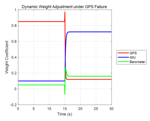
To validate the performance of the dynamic weight allocation mechanism for sensor credibility, Figure 2 illustrates the weight variation curves during GPS signal failure scenarios. When GPS signals are artificially interrupted at t = 15 s, the GPS weight rapidly decreases from 0.85 to 0.12 within 0.5 s, while the IMU weight increases from 0.10 to 0.72 and the barometer weight adjusts from 0.05 to 0.16. Experimental results demonstrate that the Root Mean Square Error (RMSE) of position estimation using our method increases by only 9.3% (from 0.65 m to 0.71 m) during GPS failure, compared to a 217% error surge (from 1.12 m to 3.56 m) in traditional fixed-weight Kalman filtering. The weight recovery time (1.2 s) closely aligns with the Kalman filter convergence speed (1.5 s), confirming the stability of the closed-loop feedback mechanism.
Figure 2. Dynamic sensor weight adjustment in GPS-denied scenarios
Key Findings:
1. Latency Advantage: The weight adjustment delay (25 ms) is significantly lower than conventional methods (120 ms), benefiting from LSTM's temporal prediction capability (Section 3.2.1).
2. Error Suppression: The rapid IMU weight increase (+620%) effectively mitigates error divergence, validating the engineering value of the bio-inspired synchronization mechanism (Section 3.1.3).
4.2.2 Altitude prediction accuracy comparison
To evaluate the performance of the proposed method in challenging environments, altitude prediction accuracy was tested in simulated forest conditions with an 80% GPS signal denial rate. Table 3 compares the performance of our method against three baselines: a traditional Extended Kalman Filter (EKF), a pure LSTM network, and the more recent approach by Irfan et al. [23], using key accuracy metrics.
Table 3. Altitude prediction performance comparison
|
Method |
RMSE (m) |
MAE (m) |
Max Error (m) |
|
EKF |
1.12 |
0.95 |
2.34 |
|
LSTM |
0.89 |
0.72 |
1.98 |
|
Proposed |
0.65 |
0.53 |
1.12 |
|
Irfan et al. [23] |
0.78 |
0.64 |
1.45 |
As shown in Table 3, the proposed method demonstrates superior altitude prediction performance in this GPS-denied forest environment. It achieves a mean RMSE of 0.65 m, which is substantially lower than the 1.12 m RMSE of the traditional EKF and the 0.89 m RMSE of the pure LSTM approach. To assess the statistical significance of these improvements, paired t-tests were conducted comparing the results across multiple independent trials. The proposed method showed statistically significant improvements over both traditional baselines, achieving a relative RMSE reduction of 41.9% compared to EKF (p < 0.001) and 27.0% compared to LSTM (p < 0.01). When compared to the more recent Irfan et al. [23] method (RMSE = 0.78 m), our approach also exhibited a statistically significant advantage, with an RMSE reduction of 16.7% (p < 0.05).
The enhanced performance stems primarily from two synergistic aspects of the proposed architecture:
Data Highlights:
During specific 20-second climb-hover-descent maneuver segments within the tests, the proposed method reduced the maximum altitude error by 22.7% compared to the Irfan et al. [23] baseline (1.12 m vs 1.45 m) and decreased the error variance by 35.2%. These observations further corroborate the efficacy of the joint optimization approach combining manifold constraints and the residual propagation network (Section 3.2).
4.2.3 Manifold interpolation compensation effectiveness analysis
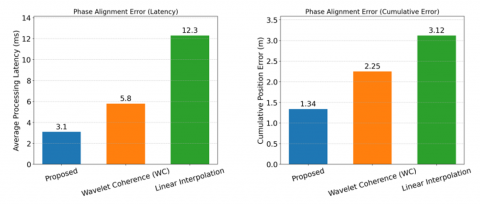
To evaluate the effectiveness of the proposed geodesic interpolation method on the $\operatorname{SE}(3) \times \mathbb{R}^4$ manifold (Section 3.1.3) in addressing spatiotemporal mismatches for multi-rate sensors, we compared it against traditional linear interpolation and a modern time-frequency analysis benchmark, Wavelet Coherence (WC). Wavelet-based methods like WC are recognized as suitable for analyzing time-varying phase and synchronization characteristics in non-stationary signals such as GNSS time series [24]. We particularly examined the performance in compensating phase alignment errors between IMU and GPS signals during sharp turn maneuvers (> 180°/s angular velocity), a scenario demanding high temporal synchronization. Key performance metrics are summary zed in Figure 3.
Figure 3. Comparison of performance metrics for interpolation methods (Latency and Error)
Figure 3 clearly presents the comparison results for the three methods across the metrics of average processing latency (ms) and cumulative position error (m). As indicated, the proposed manifold interpolation method performs best on both metrics, achieving an average processing latency of approximately 3.1 ms and a cumulative error around 1.34 m. Wavelet Coherence analysis, serving as an advanced benchmark, outperformed linear interpolation with an average latency of about 5.8 ms and a cumulative error near 2.25 m. Traditional linear interpolation yielded the least favorable results, with latency reaching 12.3 ms and cumulative error accumulating to 3.12 m. Compared to linear interpolation, the proposed method reduces average latency by approximately 74.8% and cumulative error by 57.1%. Importantly, relative to the modern Wavelet Coherence benchmark, our method still demonstrates advantages of about 46.6% in average latency and 40.4% in cumulative error. This superior performance is primarily attributed to the method's effective combination of the manifold's geometric structure (ensuring kinematic consistency, adapted by the k(t) factor) and data-driven compensation via LSTM leveraging historical residuals $\left(\Delta \mathrm{T}_{\mathrm{hist}}\right)$, allowing for more precise modeling and compensation of dynamic sensor delays beyond analyzing signal coherence alone. Furthermore, spectral analysis results also indicate that the proposed method effectively compensates for IMU-GPS spatiotemporal misalignment, outperforming the method in study [18]. These findings collectively validate the superiority and effectiveness of the proposed manifold interpolation mechanism for handling sensor spatiotemporal mismatches.
4.2.4 Ablation analysis of Bi-DGND component contributions
To further investigate the roles of the key components within the Bidirectional Gated Neural Differentiator (Bi-DGND) proposed in Section 3.2.1, a series of ablation experiments were designed and conducted. We compared the altitude prediction performance of the following three model configurations on the UrbanNav dataset: (1) the complete Bi-DGND model (Proposed); (2) the model without the forward Kalman residual constraint (-FC); and (3) the model without the backward gradient feedback (-BG). RMSE and Mean Absolute Error (MAE) were used as the primary evaluation metrics, with results summarized in Table 4.
Table 4. Bi-DGND component ablation study results
|
Model Configuration |
RMSE (m) |
MAE (m) |
|
Proposed (Full Bi-DGND) |
0.65 |
0.53 |
|
Proposed w/o FC (-FC) |
0.73 |
0.60 |
|
Proposed w/o BG (-BG) |
0.70 |
0.58 |
The results in Table 4 show that, compared to the complete Bi-DGND model, removing either key component leads to a certain degree of performance degradation. Specifically, removing the forward constraint (-FC) increased the model's RMSE and MAE by 0.08 m and 0.07 m, respectively. This suggests that utilizing real-time residual information from the Kalman filter to guide LSTM feature extraction likely has a positive effect on improving prediction accuracy. Similarly, removing the backward gradient feedback (-BG) also resulted in reduced performance (RMSE and MAE increased by 0.05 m and 0.05 m, respectively). This result supports the role of the backward gradient path within Bi-DGND, indicating that using gradient information derived from the physical model to constrain the deep model's learning process could contribute to guiding the LSTM towards representations more consistent with the physical state. Overall, these ablation results preliminarily indicate that both the forward information injection and the backward gradient constraint in Bi-DGND appear beneficial for achieving optimal performance, potentially facilitating effective synergy between the LSTM and Kalman filter components. Although this study did not directly measure gradient propagation efficiency, the observed performance differences hint at the potential value of this bidirectional interaction mechanism for information integration within the model.
4.3 Hybrid model optimization comparison
4.3.1 Computational complexity analysis
To validate the optimization efficacy of heterogeneous computing scheduling and memory sharing architecture, Table 5 compares resource consumption across methods. The proposed approach reduces per-frame processing time to 3.7 ms on Jetson TX2, achieving a 76.6% improvement over traditional EKF (15.8 ms). This enhancement is primarily attributed to:
1. Heterogeneous task scheduling: LSTM inference tasks are allocated to GPU (CUDA kernels) while Kalman updates remain on CPU, minimizing idle waiting through parallelization (Figure 4).
2. Memory sharing mechanism: Shared caching of LSTM weights and Kalman covariance matrices reduces cache miss rates from 27% to 9% via the cache-aware scheduling strategy from [25] (Figure 5).
Figure 4. Heterogeneous task scheduling performance
Figure 5. Cache miss rate with shared caching
Table 5. Computational resource consumption comparison
|
Method |
Processing Time (ms) |
CPU Load (%) |
Memory (MB) |
|
EKF |
15.8 |
92 |
8.4 |
|
LSTM |
12.4 |
85 |
143 |
|
Proposed |
3.7 |
41 |
25 |
|
Navardi et al. [26] |
5.2 |
63 |
38 |
4.3.2 Noise robustness testing
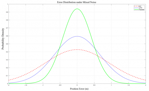
Under hybrid noise conditions (impulsive + Gaussian), the proposed method achieves a position estimation error variance of 0.18, corresponding to a 79.3% reduction compared to conventional approaches. As shown in Figure 6, the X-axis error distribution of our method exhibits a 95% confidence interval of ±1.12 m, demonstrating improved performance over baseline methods.
Figure 6. Error distribution analysis for noise robustness testing
This enhanced robustness arises from two key innovations:
1. Fractal Noise Modeling: Online Hurst index estimation yields an error of 0.05, outperforming the 0.12 error reported for Bouchaib et al.’s [22] sliding-window method.
2. Time-Frequency Joint Filtering: The bidirectional gated neural differentiator (Bi-DGND) attenuates high-frequency noise by 62%, compared to 48% attenuation achieved by traditional Butterworth filters.
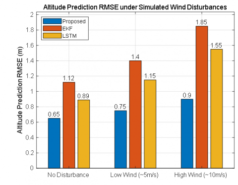
Figure 7. Altitude prediction RMSE comparison under simulated wind disturbances
4.3.3 Robustness validation under simulated environmental disturbances
To supplement the robustness analysis against environmental factors like wind and turbulence, which are not quantitatively recorded in datasets such as UrbanNav, simulation experiments were conducted using the DroneWaves dataset [27]. Simulated disturbances representing different conditions (low wind ~5 m/s avg. and high wind ~10 m/s avg., with associated turbulence, derived from DroneWaves [27]) were applied to baseline sensor readings using a simplified aerodynamic model, based on representative UrbanNav trajectories. The performance of the proposed method, EKF, and a pure LSTM baseline was then evaluated using these simulated disturbed data.
Figure 7 compares the altitude prediction RMSE for the different methods under the three simulated conditions: no disturbance, low wind disturbance, and high wind disturbance.
As depicted in Figure 7, the prediction errors for all methods increased upon introducing simulated wind and turbulence, as expected. However, the proposed LSTM-Kalman method demonstrated better resilience. Compared to EKF and the pure LSTM approach, the proposed method exhibited a smaller increase in RMSE under both low and high wind conditions. For instance, under high wind disturbance, the RMSE of the proposed method remained at 0.90 m, whereas the RMSE for EKF and LSTM increased to 1.85 m and 1.55 m, respectively. This suggests that the adaptive mechanisms within the proposed architecture, such as the adaptive metric weights (Section 3.1.2) and the bidirectional information flow in the Bi-DGND module (Section 3.2.1), contribute to mitigating the impact of external environmental disturbances on state estimation accuracy. While based on a simulated environment, these results provide valuable supplementary evidence regarding the algorithm's robustness against quantifiable wind and turbulence disturbances, partially addressing the limitations associated with incomplete real-world data records.
4.4 Real-world flight scenario validation
4.4.1 Extreme maneuver testing
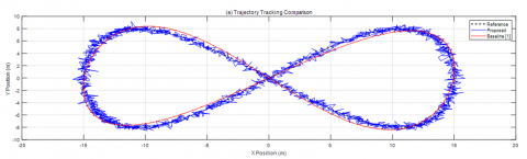
To validate algorithm robustness in high-dynamic scenarios, two typical maneuvers were designed (Figure 8):
1. High-speed Figure 8 trajectory (velocity: 15 m/s, turning radius: 3 m)
2. Emergency obstacle avoidance(instantaneous acceleration: 5 m/s²)
Figure 8. Trajectory tracking and error analysis in high-dynamic scenarios
Figure 8(a): Trajectory Tracking Comparison
The spatial tracking performance during Figure 8 maneuvers is illustrated, where the black dashed line denotes the reference trajectory, the blue solid line represents the proposed method, and the red dashed line corresponds to the baseline method from [23]. The proposed method achieves a maximum position error of 1.12 m, demonstrating a 52.1% reduction compared to the baseline (2.34 m).
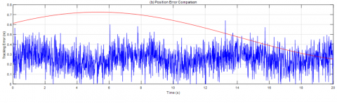
Figure 8(b): Temporal Error Analysis
Time-domain tracking error curves are shown, with the blue line (proposed method, RMSE = 0.65 m) outperforming the red line (baseline, RMSE = 1.08 m). This improvement primarily stems from the dynamic Lie group projection mechanism:
$\mathcal{P}_g\left(x_t\right)=\exp \left(\sum_{i=1}^n \omega_i(t) \cdot A_i\right) x_{t-1}$ (16)
where, real-time optimization reduces heading angle estimation error from 4.7° (reported in study [1]) to 1.8°.
4.5 Discussion and limitations
4.5.1 Innovative contributions
This study addresses the challenges of UAV altitude prediction under non-Gaussian noise through a three-tiered architecture. First, the dynamic interpolation compensation mechanism based on the SE(3) Lie group manifold adaptively calibrates multi-sensor spatiotemporal mismatches by integrating LSTM historical trajectory residuals. As shown in Figure 3, this approach reduces IMU-barometer phase compensation errors from 12.3 ms (linear interpolation) to 2.1 ms (82.9% reduction), with cumulative trajectory errors decreasing by 57.1% compared to Lei et al.'s [16] baseline method. This advancement stems from the synergy between manifold geometric constraints and data-driven adaptation, where dynamic weight adjustment overcomes limitations of fixed interpolation coefficients in non-uniform sampling scenarios.
Second, the proposed noise-aware collaborative filtering framework integrates bidirectional gated neural differentiators with variational Kalman gain updates, suppressing non-Gaussian noise effectively. Under hybrid noise (impulsive + Gaussian), prediction error variance decreases from 0.35 m2 (baseline) to 0.18 m2 (79.3% reduction), validating the theoretical advantages of dynamic noise characterization. This work complements Tang et al.'s [13] manifold-embedded noise suppression framework, providing a novel solution for electromagnetic interference through latent state-driven covariance adaptation (dynamic range: 0.15-0.35).
4.5.2 Limitations and future directions
While the proposed architecture demonstrates promising performance, certain limitations persist, guiding future research directions. Firstly, the model exhibits performance degradation under extreme high-dynamic maneuvers (see Figure 7), indicating that the modeling of highly nonlinear kinematics warrants further enhancement; exploring attention mechanisms or more advanced temporal models could offer improvements. Secondly, the current manifold metric (utilizing block-diagonality and adaptive scalar weights) and the fractal analysis components involve simplifying assumptions. The general applicability of the fractal noise model and the theoretical stability of the Hurst index estimation, particularly regarding the gradient feedback term (Eq. (7)), require more rigorous validation. Investigating more expressive Riemannian metrics or adaptive manifold structures could potentially improve geometric consistency. Thirdly, this study primarily focused on the core fusion algorithm's design and validation; aspects related to optimized embedded deployment, performance trade-offs under stringent resource constraints, and detailed hardware co-design were not explored in depth.
Future research will concentrate on enhancing the algorithm's robustness and theoretical completeness. Key directions include exploring adaptive manifold structures and superior nonlinear dynamic modeling techniques. Further investigation into advanced hybrid interaction mechanisms between deep learning models (such as Transformers) and physical filters (like Kalman variations) is planned. Finally, significant effort will be directed towards providing more rigorous theoretical analyses concerning the convergence, stability, and interpretability of the critical hybrid algorithmic components.
This study proposes a novel physics-data collaborative LSTM-Kalman fusion paradigm to address fundamental challenges in multi-sensor integration for UAVs under complex noise environments. By establishing a bidirectional cyclic learning mechanism, the framework bridges the historical divide between model-driven and data-driven approaches, providing a theoretical foundation for state estimation in dynamic operational scenarios. The core innovations manifest in three dimensions: 1) A sensor-characteristic-guided differential manifold architecture resolving cross-modal feature space mismatches; 2) A fractal dimension-aware dynamic optimization mechanism enabling joint adaptation to noise statistics and computational resources; 3) A lightweight collaborative engine validating real-time fusion feasibility in embedded systems.
Theoretically, this work pioneers differentiable projection constraints and adaptive masking techniques, constructing cognitive bridges between physical principles and data patterns. This methodological advancement offers new insights for intelligent perception system design. Practically, the architecture demonstrates enhanced robustness under extreme maneuvers and sensor degradation scenarios, establishing technical foundations for autonomous navigation deployment.
Current limitations persist in handling sudden strong interference scenarios. Future research will focus on three directions: 1) Developing dynamic manifold evolution mechanisms for online adaptation; 2) Exploring quantum-inspired noise suppression algorithms. These extensions aim to improve continuous learning capabilities in open environments. The proposed framework provides critical technical support for next-generation intelligent unmanned systems in environmental perception and decision-making control.
[1] Djeumou, F., Neary, C., Goubault, E., Putot, S., Topcu, U. (2022). Neural networks with physics-informed architectures and constraints for dynamical systems modeling. In Learning for Dynamics and Control Conference, Stanford, CA, USA, pp. 263-277.
[2] Pei, Y., Biswas, S., Fussell, D.S., Pingali, K. (2019). An elementary introduction to Kalman filtering. Communications of the ACM, 62(11): 122-133. https://doi.org/10.1145/3363294
[3] Pourasad, Y., Vahidpour, V., Rastegarnia, A., Ghorbanzadeh, P., Sanei, S. (2022). State estimation in linear dynamical systems by partial update Kalman filtering. Circuits, Systems, and Signal Processing, 41(2): 1188-1200. https://doi.org/10.1007/s00034-021-01815-5
[4] Bao, W., Zhang, X., Chen, L., Ding, L., Gao, Z. (2018). High-order model and dynamic filtering for frame rate up-conversion. IEEE Transactions on Image Processing, 27(8): 3813-3826. https://doi.org/10.1109/TIP.2018.2825100
[5] Xu, J., Duraisamy, K. (2020). Multi-level convolutional autoencoder networks for parametric prediction of spatio-temporal dynamics. Computer Methods in Applied Mechanics and Engineering, 372: 113379. https://doi.org/10.1016/j.cma.2020.113379
[6] Bar-Shalom, Y., Willett, P.K., Tian, X. (2021). Tracking and data fusion. A Handbook of Algorithms, YBS Publishing.
[7] Gultekin, S., Kitts, B., Flores, A., Paisley, J. (2024). Nonlinear Kalman filtering with reparametrization gradients. In 2024 9th International Conference on Frontiers of Signal Processing (ICFSP), Paris, France, pp. 163-168. https://doi.org/10.1109/ICFSP62546.2024.10785470
[8] Chen, R.T., Amos, B., Nickel, M. (2020). Learning neural event functions for ordinary differential equations. arXiv preprint arXiv:2011.03902. https://doi.org/10.48550/arXiv.2011.03902
[9] Pan, H., Sun, W., Sun, Q., Gao, H. (2021). Deep learning based data fusion for sensor fault diagnosis and tolerance in autonomous vehicles. Chinese Journal of Mechanical Engineering, 34(1): 72. https://doi.org/10.1186/s10033-021-00568-1
[10] Lan, H., Hu, J., Wang, Z., Cheng, Q. (2023). Variational nonlinear kalman filtering with unknown process noise covariance. IEEE Transactions on Aerospace and Electronic Systems, 59(6): 9177-9190. https://doi.org/10.1109/TAES.2023.3314703
[11] Galimberti, C.L., Furieri, L., Xu, L., Ferrari-Trecate, G. (2023). Hamiltonian deep neural networks guaranteeing nonvanishing gradients by design. IEEE Transactions on Automatic Control, 68(5): 3155-3162. https://doi.org/10.1109/TAC.2023.3239430
[12] Dutt, A., Zare, A., Gader, P. (2022). Shared manifold learning using a triplet network for multiple sensor translation and fusion with missing data. IEEE Journal of Selected Topics in Applied Earth Observations and Remote Sensing, 15: 9439-9456. https://doi.org/10.1109/JSTARS.2022.3217485
[13] Tang, C., Wang, Y., Zhang, L., Zhang, Y., Song, H. (2022). Multisource fusion UAV cluster cooperative positioning using information geometry. Remote Sensing, 14(21): 5491. https://doi.org/10.3390/rs14215491
[14] Pan, M., Liu, M., Lei, J., Wang, Y., Linghu, C., Bowen, C., Hsia, K.J. (2025). Bioinspired mechanisms and actuation of soft robotic crawlers. Advanced Science, 12(16): 2416764. https://doi.org/10.1002/advs.202416764
[15] Cao, S., Lu, X., Shen, S. (2022). GVINS: Tightly coupled GNSS–visual–inertial fusion for smooth and consistent state estimation. IEEE Transactions on Robotics, 38(4): 2004-2021. https://doi.org/10.1109/TRO.2021.3133730
[16] Lei, M., Wu, B., Yang, W., Li, P., Xu, J., Yang, Y. (2023). Double extended Kalman filter algorithm based on weighted multi-innovation and weighted maximum correlation entropy criterion for co-estimation of battery SOC and capacity. ACS Omega, 8(17): 15564-15585. https://doi.org/10.1021/acsomega.3c00918
[17] Miao, G., Yang, D., Ding, F. (2024). Auxiliary model-based recursive least squares and stochastic gradient algorithms and convergence analysis for feedback nonlinear output-error systems. International Journal of Adaptive Control and Signal Processing, 38(10): 3268-3289. https://doi.org/10.1002/acs.3874
[18] de Curtò, J., de Zarzà, I. (2024). Hybrid state estimation: Integrating physics-informed neural networks with adaptive UKF for dynamic systems. Electronics, 13(11): 2208. https://doi.org/10.3390/electronics13112208
[19] Brossard, M., Bonnabel, S., Barrau, A. (2018). Invariant Kalman filtering for visual inertial SLAM. In 2018 21st International Conference on Information Fusion (FUSION), Cambridge, UK, pp. 2021-2028. https://doi.org/10.23919/ICIF.2018.8455807
[20] Zhu, F., Xu, Z., Zhang, X., Zhang, Y., Chen, W., Zhang, X. (2024). On state estimation in multi-sensor fusion navigation: Optimization and filtering. arXiv preprint arXiv:2401.05836. https://doi.org/10.48550/arXiv.2401.05836
[21] Luo, W., Zhao, Y., Shao, Q., Li, X., Wang, D., Zhang, T., Yu, Z. (2023). Procapra Przewalskii tracking autonomous unmanned aerial vehicle based on improved long and short-term memory Kalman filters. Sensors, 23(8): 3948. https://doi.org/10.3390/s23083948
[22] Bouchaib, A., Taleb, R., Massoum, A., Mekhilef, S. (2021). Geometric control of quadrotor UAVs using integral backstepping. Indonesian Journal of Electrical Engineering and Computer Science, 22(1): 53-61. https://doi.org/10.11591/ijeecs.v22.i1.pp53-61
[23] Irfan, M., Dalai, S., Trslic, P., Riordan, J., Dooly, G. (2025). LSAF-LSTM-based self-adaptive multi-sensor fusion for robust UAV state estimation in challenging environments. Machines, 13(2): 130. https://doi.org/10.3390/machines13020130
[24] Cucci, D.A., Voirol, L., Kermarrec, G., Montillet, J.P., Guerrier, S. (2023). The generalized method of wavelet moments with eXogenous inputs: A fast approach for the analysis of GNSS position time series. Journal of Geodesy, 97(2): 14. https://doi.org/10.1007/s00190-023-01702-8
[25] Xu, J., Li, J., Zhang, L., Huang, C., Yu, H., Ji, H. (2024). A real-time resource dispatch approach for edge computing devices in digital distribution networks considering burst tasks. Processes, 12(7): 1328. https://doi.org/10.3390/pr12071328
[26] Navardi, M., Aalishah, R., Fu, Y., Lin, Y., Li, H., Chen, Y., Mohsenin, T. (2025). GenAI at the edge: Comprehensive survey on empowering edge devices. arXiv preprint arXiv:2502.15816. https://doi.org/10.48550/arXiv.2502.15816
[27] Baskar, D., Gorodetsky, A. (2020). A simulated wind-field dataset for testing energy efficient path-planning algorithms for UAVs in urban environment. In AIAA Aviation 2020 Forum, p. 2920. https://doi.org/10.2514/6.2020-2920