Selahattin Güçlü*![]() | Durmuş Özdemir
| Durmuş Özdemir![]() | Hamdi Melih Saraoğlu
| Hamdi Melih Saraoğlu![]()
© 2025 The authors. This article is published by IIETA and is licensed under the CC BY 4.0 license (http://creativecommons.org/licenses/by/4.0/).
OPEN ACCESS
Computer-aided detection of anomalies in X-ray images is of great importance and is one of the essential branches of image recognition. This research is focused on designing a deep learning (DL) architecture, DenseNet, by integrating parallel structures, utilizing humerus and shoulder X-ray datas from the MURA dataset. For detecting anomalies, AlexNet, ResNet, DenseNet, Parallel DenseNet, and the newly Mofified DenseNet (MDN) models of DL are employed, and the analysis results for the humerus and shoulder are compared. A total of 628 healthy and 643 anomalies X-ray images for the humerus, along with 1505 healthy and 1530 anomalies X-ray images for the shoulder, were utilized to train the models DL. The statistical analysis for the humerus revealed that the Modified DenseNet model was the most successful, achieving a test accuracy of 78.65%. The next most successful model was AlexNet, with a test accuracy of 72.4%. The statistical analysis for the shoulder indicated that the most effective model, based on test accuracy, was the Modified DenseNet model with a score of 68.42%, followed by AlexNet with a score of 67.54%. In anomaly identification using musculoskeletal humerus and shoulder X-ray datas, the DenseNet-based MDN architecture was more successful in test accuracy than the traditional DenseNet model. This success in test accuracy rates will support those studies in this field.
DenseNet, deep learning, convolution layer
Bones are among the most crucial components of the human body. In the human body, bones facilitate movement and allow individuals to carry out various life functions. Additionally, bones provide the first line of protection for the body's soft tissues through structures like the rib cage, skull, and other components. Bones are the densest natural structures in terms of composition. However, any change in the composition of the structure and shape of bones tends to render them unable to perform human functions in their natural form [1]. Fractures, a common type of orthopedic trauma, can affect individuals of all ages. These injuries often result from high-impact incidents such as severe falls, car accidents, or prolonged load-bearing stress on otherwise healthy bones [2]. Therefore, this change is called an anomaly. The primary causes of these anomalies include genetic factors, direct injuries, and infections affecting the bone and muscle structures [1]. X-ray images of the musculoskeletal system are vital for anomaly classification. Generally, when a patient experiences an accident or suspects a fracture, they visit the emergency room, where the doctor initially takes an X-ray to identify any fractures. X-ray images can be misclassified in the emergency department. This is because the process is fast, and the emergency room doctor classifying the X-ray is not an experienced radiologist, which can lead to an unexpected misdiagnosis [3]. As a result, a doctor's experience may lead to missed detection of various anomalies, such as fractures, hardware, subluxations, degenerative joint disease and lesions [4]. In the classification of X-ray images, having an automatic classifier can be very helpful to the doctor and reduce the error rate [3]. The computer processing and analysis of X-ray images involve image formation, image acquisition, image-based visualization, and image analysis. X-ray image processing has expanded to encompass pattern recognition, computer vision, image mining, and various aspects of machine learning. DL is a commonly employed approach for image classification. [5]. DL for medical image classification typically relies on well-annotated datasets for training, which strongly motivates research institutions and hospitals to develop medical datasets [6].
When studies on the detection of musculoskeletal anomalies in humans are examined, X-ray datas of patients are used as data sets. DL algorithms operate with these data sets.
Avcı and Alzabaq [7] applied a DL approach using a Convolutional Neural Network (CNN) on a radiography dataset to identify COVID-19. The proposed system comprises multiple stages, beginning with preprocessing, followed by feature reduction using various techniques, and concluding with classification based on the proposed model. Urakawa et al. [8] utilized transfer learning for anomaly classification on cropped front-view hip radiographs using the pre-trained VGG16 classification model. Harini et al. [9] compared the results using Xception, VGG-19, Inception V3, MobileNet, and DenseNet DL methods using the MURA (Musculoskeletal Radiographs) dataset's finger, wrist, and shoulder X-ray images. Barhoom et al. [1] modified the VGG-16 DL method for anomaly detection in all parts of the MURA dataset. Nguyen et al. [10] used a YOLOV4-based DL method for anomaly detection in X-ray datas. In addition to using some data augmentation techniques during training, they also showed the effect of image contrast algorithms on performance. Faster-Recurrent Convolutional Neural Networks (RCNN)-based classification has been reported to give better results. Alzubaidi et al. compared a new transfer learning model with traditional DL methods using shoulder X-ray datas in the MURA dataset and stated that they got better results in their proposed model [11]. Manoila et al. [12] presented a flexible MRI analysis framework with various DL models with preset parameters for automatically identifying the knee joint region. Spotlights a promising CNN designed for knee bone segmentation alongside a novel weighted subsampling technique to enhance image processing.
Interpretation of medical imaging examinations is a complex cognitive and psychophysiological process with a high potential for error. A trained radiologist has an error rate of approximately 4% in the image interpretation process. Since approximately 1 billion radiologic imaging evaluations are performed annually, this equates to approximately 40 million radiologist errors annually [13].
Kazemi et al. [14] analyzed medical images, especially those used to diagnose brain diseases, with CNN, one of the DL methods. Their proposed method is a profound parallel convolutional neural network model that includes AlexNet and VGGNet networks. The layer structures of these two networks are different, and the features are combined at one point and classified using the SoftMax function. This proposed parallel structure achieved better results than existing models. Rezaoana et al. [15] used parallel layers using VVG DL algorithms for skin cancer detection in their study. Their proposed method obtained more successful results than the classical VVG DL algorithm. The DenseNet method was prone to adding parallel blocks, and successful predictions would be made in X-ray images.
In the literature studies, the DenseNet has successful results, is DL method, in human musculoskeletal disorders. There are DL algorithms with multi layers. For collections containing numerous X-ray images, like the MURA dataset, the performance evaluation of parallel layers and the impact of increasing the number of layers remain underexplored. In this study, a parallel and multilayerstructure is hypothesized based on existing literature to enhance accuracy performance and is tested by implementing it within the traditional DenseNet framework. The layers of the traditional DenseNet DL model were modified into parallel connections as blocks. Performance analysis of test accuracy values was conducted compared to the AlexNet, ResNet and other DenseNet models. The study suggests that the MDN model should be applied in a way that allows the detection of musculoskeletal anomalies when compared to the traditional DenseNet model.
This study was designed and organized as follows: Part 2 provides information on DL architecture and technical procedures used. The modified models, processes, and evaluation criteria are explained in Part 3. Experimental analysis and results are detailed in Part 4, and concluding comments and recommendations are in Part 5.
2.1 Deep learning (DL)
DL is a categorized under machine learning that focuses on algorithms designed to represent high-level abstractions in data through a series of non-linear transformations. These transformations are constructed using sophisticated structures, notably neural network structures [16]. The algorithm used in DL is a neural network with multiple hidden layers [17]. Inspired by the human brain, it has emerged due to studies to produce more intelligent systems. In the 1940s, S. McCulloch and Walter H. Pitts discussed that the activity or inactivity of neurons in the brain depends on a threshold value. They suggested that neurons in the brain could be connected to form a circuit, and decisions could be made with this circuit. The weighted total is obtained by multiplying the neurons' inputs by specific coefficients. The result is compared to a threshold value. If the result is below the threshold value, it will not move to the next layer, but if it exceeds the threshold value, it will move to the next layer. This structure mainly illustrates the working principle of artificial neural networks [18]. The concept of multilayer artificial neural network structure led to the development of CNN by increasing the number of layers. Computer technology advances have also significantly contributed to the resurgence of artificial neural networks [19].
DL can be performed as supervised, unsupervised, semi-supervised, or reinforcement learning. The learning process is called deep because artificial neural networks in this structure typically consist of multiple input, output, and hidden layers. Through these layers, information is accessed by processing the data. DL needs a vast dataset for training to ensure precise predictions.
Unlike traditional machine performance, DL is more efficient at more complex operations on machines with high-end hardware. Another difference from machine learning is that the output of DL does not have to be a classification or a numerical value. In addition to producing a numeric value at the output layer, it can produce multi-format outputs such as audio and text. DL can be used in many different sectors. Examples of the most common areas of use are image processing classification, audio signal classification or noise reduction, sentiment analysis, chatbots, self-driving vehicles, automatic recommendations for services, making predictions to help diagnosis and treatment in the medical sector, etc. [20, 21].
We can classify commonly used DL structures today as follows: Deep Auto-Encoders, Generative Adversarial Networks (GAN), Convolutional Neural Networks (CNN), Recurrent Neural Networks (RNN), Hybrid Architectures (HA) and Deep Belief Networks [22]. Since the MURA dataset consists of images, the CNN model will be used because it is successful in image processing.
2.2 Models
CNN, a DL method, is one of the leading algorithms used in image recognition in healthcare due to its robust feature extraction capability [23]. Convolutional Neural Networks excel in image recognition tasks due to their ability to capture and learn hierarchical features from input data [24]. This study used AlexNet, ResNet and DenseNet DL methods, which are famous for training with CNNs, to train humerus and shoulder X-ray images.
2.2.1 AlexNet model
The AlexNet model, widely used in transfer learning applications, was developed by Alex et al. [25]. This DL model was developed by training over 1 million images across 1000 diverse classes (including animals, plants, etc.) from the ImageNet database. The image input dimensions are specified as 227×227×3. The model comprises 25 layers, with approximately 60 million parameters computed. The model uses five convolutional layers, three pooling layers, 7 ReLU (Rectified Linear Unit) activation function layers, and three fully connected layers. Using transfer learning methods from AlexNet, pre-trained parameters enable better classification of smaller datasets [26]. The structural design of AlexNet is shown in Figure 1.
Figure 1. The structural design of the AlexNet DL model [27]
2.2.2 ResNet model
The Residual Network (ResNet) structure is a crucial DL approach known for its effectiveness in handling complex tasks like image classification with high performance. This type of network is designed to create deeper and more complex structures. Due to their multilayer structure, deep neural networks can face the "vanishing gradient" problem. This means the network gradient approaches zero, slowing the learning process. Since the gradient is multiplied at each layer during backpropagation, in deep networks, this gradient can quickly drop to zero. To contribute to the learning process, a shortcut called a "skip connection" is added. This connection helps to pass information from one layer to another more efficiently and allows data to bypass the standard convolutional neural network flow. ResNet has many variants with different number of layers. For example, ResNet18, ResNet34, ResNet50, ResNet101 and ResNet152. In our study, the ResNet18 model was used to keep the training time short. Figure 2 shows the ResNet18 structure.
Figure 2. The structural design of the ResNet DL model [28]
ResNet18 consists of 18 layers with a core size of 7×7. Each layer contains two residue blocks, each with two weight layers. The input dimension is set to (224, 224, 3), representing the images' width, height, and RGB (red, green, blue) channels. An additional layer was incorporated at the end of ResNet18 to enhance the model's accuracy. This layer includes a linear (512, 512) layer, a ReLU activation function, a dropout (0.2) layer, and finally, a structure that results in SoftMax [29].
2.2.3 DenseNet model
DenseNet, improved by Yan et al. [30] builds on the hypothesis that dense connections between initial and subsequent layers in CNN models can significantly enhance Accuracy and efficiency. DenseNet consists of fully connected layers, where each layer is connected to every subsequent layer in contrast to the traditional CNN model. In a regular k-layer CNN, there are k connections, whereas in the DenseNet model, each layer is connected to each subsequent layer, so there is k(k+1)/2 connections. In the In the DenseNet DL model, every layer takes the feature maps from all previous layers as input, and its own feature maps are subsequently forwarded to the next layers [31]. In this way, DenseNet aims to address the gradient issue, promotes the reuse of features, enhances feature propagation, and substantially minimizes the number of parameters [32]. There are types of DenseNet with 121, 169, 201, and 264 layers [33]. Figure 3 illustrates the structural design of the DenseNet model. The structures vary based on the different types of DenseNet, and these variations are presented in Table 1. These differences are due to the different number of layers of DenseNet types.
Figure 3. The structural design of the traditional DenseNet DL architecture [34]
Table 1. Structures of DenseNet. (convl = Batch Normalization (BN)+ReLU+convolution layers [35]
|
Layers |
Output Size |
DenseNet-121 |
DenseNet-169 |
DenseNet-201 |
DenseNet-264 |
|||||||
|
Convolution |
112×112 |
(stride 2), 7×7 conv |
||||||||||
|
Pooling |
56×56 |
(stride 2), 3×3 max pool |
||||||||||
|
1. Dense Block |
56×56 |
1×1 convl 3×3 convl |
×6 |
1×1 convl 3×3 convl |
×6 |
1×1 convl 3×3 convl |
×6 |
1×1 convl 3×3 convl |
×6 |
|||
|
1. Transition Layer |
56×56 |
1×1 convl |
||||||||||
|
28×28 |
(stride 2), 2×2 average poo |
|||||||||||
|
2. Dense Block |
28×28 |
1×1 convl 3×3 convl |
×12 |
1×1 convl 3×3 convl |
×12 |
1×1 convl 3×3 convl |
×12 |
1×1 convl 3×3 convl |
×12 |
|||
|
2. Transition Layer |
28×28 |
1×1 convl |
||||||||||
|
14×14 |
(stride 2), 2×2 average pool |
|||||||||||
|
3. Dense Block |
14×14 |
1×1 convl 3×3 convl |
×24 |
1×1 convl 3×3 convl |
×32 |
1×1 convl 3×3 convl |
×48 |
1×1 convl 3×3 convl |
×64 |
|||
|
3. Transition Layer |
14×14 |
1×1 convl |
||||||||||
|
7×7 |
(stride 2), 2×2 average pool |
|||||||||||
|
4. Dense Block |
7×7 |
1×1 convl 3×3 convl |
×16 |
1×1 convl 3×3 convl |
×32 |
1×1 convl 3×3 convl |
×32 |
1×1 convl 3×3 convl |
×48 |
|||
|
Classification Layer |
1×1 |
7×7 global average pool |
||||||||||
|
|
1000D fully-connected and softmax |
|||||||||||
In Figure 4, the structure of the DenseNet block expansion is shown. This densely connected structure of DenseNet makes it possible to create deeper networks with fewer parameters, thus increasing the model's generalization ability and accelerating the learning process.
Figure 4. DenseNet block expansion [36]
Figure 5 shows the structure of the DenseNet transition layer expansion. Transition layers are critical components that make DenseNet an efficient and powerful model. These layers ensure a balanced and controlled flow of information between dense blocks.
Figure 5. DenseNet transition layer expansion [36]
DenseNet-264 improves information flow and gradient propagation thanks to its densely connected structure, which enables deeper networks to learn more efficiently and effectively. This structure is ideal for achieving high performance on large and complex datasets. The traditional DenseNet model, DenseNet-264, was utilized in the study to analyze radiography images in the MURA dataset.
The Dense Block is at the centre of the DenseNet model and ensures that all layers are interconnected. In this way, the outputs of the previous layers are used as inputs to all subsequent layers. These dense connections minimise the information loss of the model and ensure that important features are captured efficiently. However, optimization is possible, as the arrangement of the different functional layers within the Dense block module could be made more efficient. In the CrodenseNet structure, improved results in diagnosing COVID-19 have been obtained by employing various parallel structures [37]. Yin et al. [38] achieved favorable results by applying parallel layers to the traditional DenseNet model, using the image datasets. Unlike Yin et al. [38], who employed three parallel blocks by decreasing the number of traditional DenseNet blocks, this study utilized four parallel DenseNet blocks. Therefore, by removing, adding, and adjusting convolutional layers and adding parallel blocks, the DenseNet DL method has been improved. When more convolution layers are superimposed on the receiver field, which is more significant, it can enable more prosperous feature extraction and over computational efficiency. Unlike Yin et al. [38], the improved DenseNet models of DL use a 3×3 convolution layer instead of a 1×1 layer to capture or extract features from larger regions. The 3×3 convolution layer analyzes each pixel along with the pixels in a 3×3 window surrounding it.
DenseNet uses a single convolutional filter to extract features from the input image. Then, these features are forwarded to the dense block module. This leads to a relatively simple structure, which may result in the loss of image information [38]. A novel dilated convolution block, was developed in parallel to maximize the utilization of current features without significantly increasing the number of parameters. Subsequently, multi-path Dense blocks are integrated to merge diverse feature maps originating from various paths. Hence, facilitates the harmonization of channel features and enables robust feature extraction.
In this research, to improve a DL model utilizing X-ray radiography from the dataset of MURA, a new model named 'Canonical Parallel DenseNet' was created by incorporating Dense blocks in parallel with the traditional DenseNet structure. Implementing parallelism in the DenseNet structure resulted in improved classification performance [37, 38]. This Parallel DenseNet structure underwent optimization, leading to the creation of the 'Modified DenseNet' model. The DenseNet models in this study are trained and subsequently employed for image recognition process. Furthermore, the accuracy of this MURA X-ray image detection is assessed by analyzing the results with the labeled dataset.
3.1 Canonical Parallel DenseNet model
Inside the canonical parallel DenseNet architecture created using the traditional DenseNet 264 model, the layer configuration and the number of repetitions are preserved. The transition layers are identical to those depicted in Figure 5. The structural design of the parallel DenseNet DL model is illustrated in Figure 6.
As illustrated in Figure 6, additional Dense blocks, mirroring the layers and features of the traditional Dense blocks, are integrated in parallel to the existing structure of the traditional DenseNet structure. These Dense block numbers can be increased and decreased [38]. Parallel blocks retain the same characteristics as those in the traditional DenseNet structure. These blocks are interconnected using transition layers. Due to the parallel connections, Dense blocks are connected by merging their feature maps, and feature extraction is performed. In the last layer, the 'Pooling-Full Connection' layers are linked to classify 'Anomaly - Healthy.' Due to a decrease in performance with a 10% drop in test accuracy in analyses conducted by three parallel modules, the number of parallel Dense modules was changed to be four.
Figure 6. The structural design of the parallel DenseNet DL model
3.2 Modified DenseNet model
Inside the MDN architecture, the layers and iteration count from the traditional DenseNet-264 structure were replicated exactly. Transition layers are the identical to given in Figure 5. In the modified architecture, an structure is formed by connecting enhanced Dense blocks with discrete Dense blocks in parallel, as shown in Figure 7.
Figure 7. The structural design of the MDN DL model
Traditional DenseNet structure consists of successively added layers. In the MDN structure, parallel modules were linked using transition layers that retain the equivalent characteristics as those in the traditional DenseNet, as illustrated in Figure 7. Dense modules integrate feature maps from different ways and then assist in feature extraction. The improved DenseNet architecture description is given in Figure 8.
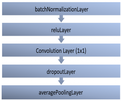
As given in Figure 8, different from the traditional DenseNet block (Figure 4), to preserve the information in the X-ray, in the improved DenseNet block expansion, the convolution layers are used as 3×3 instead of 1×1. The traditional DenseNet block has a 6-layer structure, and the blocks are connected in series. In contrast to the traditional Dense block, layers consisting of Batch Normalization, ReLU, and Convolution have been sequentially incorporated.
Figure 8. Expansion of the improved DenseNet block
Figure 9 illustrates the expansion of the discrete DenseNet block. With the developed DenseNet block, the number of layers was increased to 10. The purpose of increasing the number of layers is to enable DenseNet to learn and perform effectively. As the depth of the model increases, the combination of components optimizes the learning and generalization ability.
Figure 9. Discrete DenseNet block expansion
In the MDN structure, as depicted in Figure 9, the parallel-connected Discrete DenseNet block expansion employs 3×3 convolution layers instead of 1×1 to preserve image information, unlike the traditional Dense block shown in Figure 4. Additionally, a Batch Normalization layer is included to facilitate normalization. Prior to the classification layer, in contrast to the traditional DenseNet structure, 'Anomaly-Healthy' classification is achieved through the use of Batch Normalization, ReLU, Convolution, and dropout layers.
In the parallel DenseNet model, the traditional DenseNet block layers in Figure 4 were connected in parallel. In the MDN model, improved (Figure 8) and discrete DenseNet (Figure 9) blocks were connected in parallel.
The parallel structure of the MDN model is qualify the fact that every layer is linked to all preceding layers. This enables each layer to reuse and preserve features from all previous layers. This connection model allows the network to learn more efficiently and perform better. This structure of the MDN is realized through structures that connect all layers directly when the sizes of the feature maps match. This minimizes information loss and allows gradients to flow better, even in the deeper layers of the network.
3.3 Dataset and image preprocessing
The MURA dataset is a large dataset consisting of X-ray images collected from a wide range of patients over an extended period. The MURA dataset comprises images sourced from the Picture Archive and Communication System (PACS) of Stanford Hospital, ensuring compliance with Health Insurance Portability and Accountability Act (HIPAA) standards [39]. The dataset consists of seven types of bones, including forearm, elbow, wrist, humerus, hand, fingers, and shoulder. This massive dataset has been collected from 12,173 patients, containing 40,561 X-ray images with multiple views of different anatomical positions [40]. Radiologists manually labeled the entire data set as healthy or anomalous [41]. The distribution of the dataset by regions is presented in Table 2.
Table 2. MURA dataset distribution [42]
|
Region |
Train |
Validation |
||
|
Healthy |
Anomaly |
Healthy |
Anomaly |
|
|
Wrist |
5765 |
3987 |
364 |
295 |
|
Shoulder |
4211 |
4168 |
285 |
278 |
|
Forearm |
1164 |
661 |
150 |
151 |
|
Humerus |
673 |
599 |
148 |
140 |
|
Finger |
3138 |
1968 |
214 |
247 |
|
Elbow |
2925 |
2006 |
234 |
230 |
|
Hand |
4059 |
1484 |
271 |
189 |
Anomaly detection involves a binary classification process to distinguish between healthy studies and those with anomalies. Identifying whether an X-ray image is healthy or anomaly is crucial because it can help rule out the need for additional, procedures, diagnostic tests, and interventions for patients. The causes of the anomaly are listed as various abnormalities, such as degenerative joint diseases, hardware, fractures, lesions, and subluxations [43]. Figures 10 and 11 present the humerus and shoulder regions of the X-ray MURA dataset.
Figure 10. MURA dataset humerus region (a) healthy, (b) anomaly dataset example [44]
Figure 11. MURA dataset shoulder region (a) healthy, (b) anomaly dataset example [44]
The MURA dataset image sizes vary between 512×512 pixels and 97×512 pixels, and the file extension is '.png' [45]. In DL, to minimize input data loss and ensure uniformity of pixel values, all changeable-sized X-ray datas were image adjusted to 320×320 pixels [46]. After the pixel change, '.png' images were centered and aligned by cropping out excess space or edges, as shown in Figure 10 and Figure 11. This process was performed to remove empty or unnecessary areas on the edges to bring the image closer to the region of interest or focal point. The images in the MURA dataset have a bit depth ranging from 8 to 24. The study converted the input image data’s bit depth to 8 for more efficient training [47].
The input image data was randomly rotated vertically and horizontally between -300 and +300 and projected in both x-y axes [4]. Additionally, the input X-ray was scaled between 0,9 and 1,1 to increase the number of input data [48].
The number of X-ray image data used for experimental analysis is given Table 3.
Table 3. The number of MURA X-ray image data used in the study
|
Study |
Region |
Healthy |
Anomaly |
|
Our study |
Humerus |
628 |
643 |
|
Madan et al. [49] |
Humerus |
389 |
338 |
|
Chawla and Kapoor [50] |
Humerus |
821 |
739 |
|
Our study |
Shoulder |
1505 |
1530 |
|
Kavitha et al. [51] |
Shoulder |
4394 |
4349 |
|
Reddy and Cutsuridis [52] |
Shoulder |
170 |
164 |
3.4 Evaluation criteria
In the MURA dataset, the performance of models for healthy anomaly detection was evaluated using clinically significant statistical metrics such as accuracy, precision, recall, specificity, F1-score, Cohen's kappa score, and 5-fold cross-validation. These metrics are briefly defined as follows:
3.4.1 Accuracy
Accuracy is calculated by the formula is:
Accuracy = (TN + TP) / (FN + FP + TN+ TP) (1)
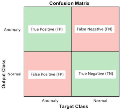
In this context, respectively; TN: denotes the count of true negative cases accurately estimated by the architecture, TP: denotes the count of true positive cases accurately estimated with the architecture, FN: denotes the count of false negative cases incorrectly estimated by the architecture, FP: denotes the count of false positive cases incorrectly estimated by the architecture.
3.4.2 Precision
The proportion of the samples that we predict are positive, and how many of them are correctly predicted? The formula is as follows.
Precision = TP / (FP + TP) (2)
3.4.3 Recall
Recall indicates how many of the samples that should be predicted positive are proportionally correctly estimated. The formula is as follows.
Recall = TP / (TP+FN) (3)
3.4.4 Specificity
The proportion of correctly identified negative instances out of all actual negative instances.
Specificity = TN / (TN+FP) (4)
3.4.5 F1-Score
F1 score combines recall and values and precision reduces them to a single number. We use the F1 score to select the best model when we have the precision and Accuracy of multiple models. The formula is as follows [53, 54].
F1-Score = 2(PrecisionxRecall) / (Precision+Recall) (5)
The confusion matrix is shown in Figure 12.
Figure 12. Confusion matrix
3.4.6 Cohen’s Cappa statistic
Cohen’s Cappa statistic ($\mathcal{K}$) is a measure used to determine the degree of harmony between two raters scoring at the classification level. ($\mathcal{K}$) value is shown formula 7 [55].
$\begin{aligned} & P_e=\frac{(F P+T P) \times(F N+T P)+(F N+T N) \times(F P+T N)}{(T N+T P+F N+F P)^2}\end{aligned}$ (6)
$\kappa=($ Accuracy-Pe) $/(1-\mathrm{Pe})$ (7)
3.4.7 K-fold cross-validation
K-fold cross-validation means the data is randomly divided by k numbers, and a different set of data is used as test data each time. In this way, all data is ensured to be used as training and test data [56]. This method, which helps to prevent the overfitting problem, is generally used in the literature for k = 3, 5, and 10 values [57]. In the study, the k value was selected as 5.
The experiments run with a laptop with a 2.30 GHz 12th Gen Intel(R) i7-12650H Core(TM) processor, running Windows 11 Pro, an NVIDIA GeForce RTX 4060 Laptop GPU and equipped with 16 GB of memory utilizing MATLAB for implementation.
The parameter configurations for the experiment are as follows: All networks used consistent settings, with a learning rate of 0.001, a minibatch size of 128, and 250 epochs. The ADAM (Adaptive Moment Estimation) algorithm was employed to minimize the error between the model's output and the actual values using the categorical cross-entropy function. This approach aimed to reduce the discrepancy between the model's predictions and the true values. The dataset was divided into 80% for training, 15% for testing and 5% for validation, with randomized allocation of images across these categories.
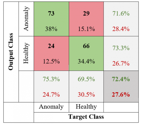
The MURA X-ray image dataset used 628 healthy and 643 anomaly images for the humerus region. The confusion matrix for the test data obtained using the AlexNet model of the humerus region is depicted in Figure 13.
Figure 13. AlexNet confusion matrix of the humerus region
The AlexNet model for the humerus region using, 73 out of 102 images labeled as anomalies were correctly identified as true positives (TP), while 29 were incorrectly identified as false negatives (FN). Among 90 images labeled as healthy, 24 were misidentified as false positives (FP), and 66 were correctly identified as true negatives (TN).
The confusion matrix for the test data obtained using the ResNet model of the humerus region is depicted in Figure 14.
Figure 14. ResNet confusion matrix of the humerus region
The ResNet model for the humerus region using, 68 out of 113 images labeled as anomalies were accurately identified as true positives (TP), while 45 were incorrectly identified as false negatives (FN). Among 79 images labeled as healthy, 29 were misidentified as false positives (FP), and 50 were correctly identified as true negatives (TN).
The confusion matrix for the test data obtained using the DenseNet model of the humerus region is depicted in Figure 15.
Figure 15. DenseNet confusion matrix of the humerus region
The DenseNet model for the humerus region using, 58 out of 84 images labeled as anomalies were correctly identified as true positives (TP), while 26 were incorrectly identified as false negatives (FN). Among 108 images labeled as healthy, 39 were misidentified as false positives (FP), and 69 were correctly identified as true negatives (TN).
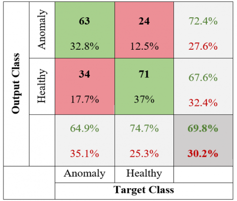
The confusion matrix for the test data obtained using the Parallel DenseNet model of the humerus region is depicted in Figure 16.
Figure 16. Canonical Parallel DenseNet confusion matrix of the humerus region
The canonical parallel DenseNet model for the humerus region using, 63 out of 87 images labeled as anomalies were accurately identified as true positives (TP), while 24 were incorrectly identified as false negatives (FN). Among 105 images labeled as healthy, 34 were misidentified as false positives (FP), and 71 were correctly identified as true negatives (TN).
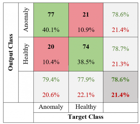
The confusion matrix for the test data obtained using the MDN model of the humerus region is depicted in Figure 17.
Figure 17. MDN confusion matrix of the humerus region
The MDN model for the humerus region using, 77 out of 98 images labeled as anomalies were correctly identified as true positives (TP), while 21 were incorrectly identified as false negatives (FN). Among 94 images labeled as healthy, 20 were misidentified as false positives (FP), and 74 were correctly identified as true negatives (TN).
Table 4 presents the comparation of DL models humerus region.
Table 4. Comparative performance of DL models for the humerus region
|
Models |
Accuracy (%) |
Specificity (%) |
Recall (%) |
F1-Score (%) |
Precision (%) |
Kappa Score |
5-fold Accuracy (%) |
Training Time (min) |
|
AlexNet |
72.40 |
73.33 |
71.57 |
73.37 |
75.26 |
0.4476 |
70.76 |
21 |
|
ResNet |
61.46 |
63.29 |
60.18 |
64.76 |
70.10 |
0.2277 |
59.04 |
245 |
|
DenseNet |
66.15 |
63.89 |
69.05 |
64.09 |
59.79 |
0.3238 |
64.86 |
67 |
|
Parallel DenseNet |
69.79 |
67.62 |
72.41 |
68.48 |
64.95 |
0.3964 |
67.45 |
254 |
|
MDN |
78.65 |
78.72 |
78.57 |
78.97 |
79.38 |
0.5728 |
77.25 |
333 |
According to Table 4, the MDN model has the highest accuracy rate (78.65%), while the ResNet model has the lowest accuracy rate (61.46%). The AlexNet model (72.4%) has a better test accuracy rate compared to DenseNet (66.15%) and Parallel DenseNet (69.79%). When the MDN architecture model test accuracy value is compared, the AlexNet model has a low value.
The MURA X-ray dataset used 1505 healthy and 1530 anomaly images for the shoulder region. The confusion matrix for the test data obtained using the AlexNet model of the shoulder region is depicted in Figure 18.
Figure 18. AlexNet confusion matrix of the shoulder region
The AlexNet model for the shoulder region using, 187 out of 292 images labeled as anomalies were accurately identified as true positives (TP), while 105 were incorrectly identified as false negatives (FN). Among 164 images labeled as healthy, 43 were misidentified as false positives (FP), and 121 were correctly identified as true negatives (TN).
The confusion matrix for the test data obtained using the ResNet model of the shoulder region is depicted in Figure 19.
Figure 19. ResNet confusion matrix of the shoulder region
The ResNet model for the shoulder region using, 136 out of 249 images labeled as anomalies were accurately identified as true positives (TP), while 113 were incorrectly identified as false negatives (FN). Among 207 images labeled as healthy, 94 were misidentified as false positives (FP), and 113 were correctly identified as true negatives (TN).
The confusion matrix for the test data obtained using the DenseNet model of the shoulder region is depicted in Figure 20.
Figure 20. DenseNet confusion matrix of the shoulder region
The DenseNet model for the shoulder region using, 162 out of 302 images labeled as anomalies were accurately identified as true positives (TP), while 140 were incorrectly identified as false negatives (FN). Among 154 images labeled as healthy, 68 were misidentified as false positives (FP), and 86 were correctly identified as true negatives (TN).
The confusion matrix for the test data obtained using the Parallel DenseNet model of the shoulder region is depicted in Figure 21.
Figure 21. Parallel DenseNet confusion matrix of the shoulder region
The canonical parallel DenseNet model for the shoulder region using, 178 out of 312 images labeled as anomalies were correctly identified as true positives (TP), while 134 were incorrectly identified as false negatives (FN). Among 144 images labeled as healthy, 52 were misidentified as false positives (FP), and 92 were accurately identified as true negatives (TN).
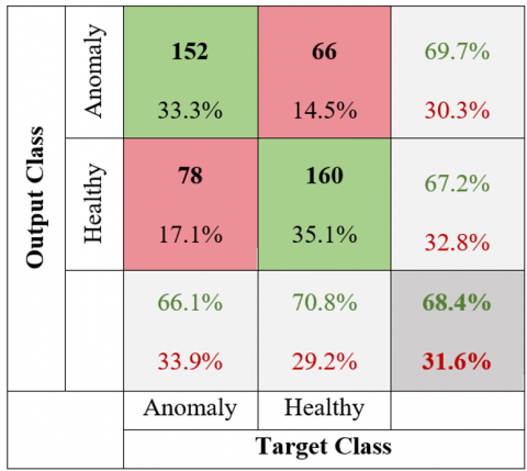
The confusion matrix for the test data obtained using the MDN model of the shoulder region is depicted in Figure 22.
Figure 22. MDN confusion matrix of the shoulder region
The MDN model for the shoulder region using, 152 out of 218 images labeled as anomalies were accurately identified as true positives (TP), while 66 were incorrectly identified as false negatives (FN). Among 238 images labeled as healthy, 78 were misidentified as false positives (FP), and 160 were correctly identified as true negatives (TN).
Table 5 presents comparation of DL models shoulder region.
According to Table 5, the MDN model has the highest accuracy rate (68.42%), while the DenseNet model has the lowest accuracy rate (54.39%). The AlexNet model (67.54%) has a better test accuracy rate compared to ResNet (54.61%) and Parallel DenseNet (59.21%). When the MDN architecture model test accuracy value is compared, the AlexNet model has a low value.
Table 5. Comparative performance of DL models for the shoulder region
|
Models |
Accuracy (%) |
Specificity (%) |
Recall (%) |
F1-Score (%) |
Precision (%) |
Kappa Score |
5-fold Accuracy (%) |
Training Time (min) |
|
AlexNet |
67.54 |
73.78 |
64.04 |
71.65 |
81.30 |
0.3493 |
65.42 |
50 |
|
ResNet |
54.61 |
54.59 |
54.62 |
56.78 |
59.13 |
0.0914 |
51.88 |
585 |
|
DenseNet |
54.39 |
55.84 |
53.64 |
60.90 |
70.43 |
0.0851 |
53.47 |
182 |
|
Parallel DenseNet |
59.21 |
63.89 |
57.05 |
65.68 |
77.39 |
0.1816 |
55.21 |
644 |
|
MDN |
68.42 |
67.23 |
69.72 |
67.86 |
66.09 |
0.3687 |
67.32 |
841 |
With the CNN models used in DL, the MURA dataset was classified as healthy and anomalous using X-ray datas of the humerus and shoulder. In this study, the traditional DenseNet model was improved, and its test results were evaluated against those of alternative models.
Using the AlexNet model, Yang and Ding [58] achieved a classification accuracy of 73.34% for the humerus region in their study. In their study, Yang et al. [59] achieved classification accuracy of 71.92% for the humerus region using the AlexNet model. These numbers are nearly match the 72.4% value obtained due to the AlexNet evaluation in this study. In their study, Kandel et al. [60] succeed a classification accuracy of 54.28% for the humerus region using the ResNetNet model. The results are similar to the 61.46% accuracy obtained from the ResNet evaluation in this study. The Kappa score (κ) of 0.5728 achieved by the MDN model demonstrated superior performance compared to all other models. During evaluations employing the 5-fold cross-validation technique, the MDN model achieved a superior accuracy of 77.25%, surpassing other models. The results test accuracy for the humerus region, the highest value (78.65%) was recorded with the MDN model, whereas the lowest accuracy (61.46%) was observed with ResNet. When we compared our AlexNet model (72.4%) results with DenseNet and canonical parallel DenseNet models, we found that we obtained a more successful result.
Yang and Ding [58] reported a classification accuracy of 68.31% for the shoulder region using the AlexNet model in their research. Similarly, Yang et al. [59] in their study achieved a classification accuracy of 67.55% for the shoulder region using the AlexNet DL model. These results are similar to the 67.54% accuracy obtained from the AlexNet analysis in this study. In their work, Kandel et al. [60] achieved a classification accuracy of 50.11% for the shoulder region using the ResNet model. In this study, this is similar to the 54.61% accuracy obtained from the ResNet analysis. The Kappa score (κ) of 0.3687 for the MDN architecture indicates better performance compared to other architectures. During the evaluations using the 5-fold cross-validation method, the MDN model demonstrated superior performance with an accuracy rate of 67.32%. According to the statistical analysis for the shoulder region, while the ResNet model had the lowest accuracy rate of 54.39% the MDN model achieved the highest test accuracy rate of 68.42%.
Furthermore, for the shoulder region, the AlexNet model (67.54%) demonstrated better performance compared to the DenseNet and Parallel DenseNet models. While Kandel et al. [60] reported an accuracy of 70.54% for the humerus region using the traditional DenseNet model, the test accuracy of the MDN architecture in our study was higher at 78.65%. Furthermore, Harini et al. [9] achieved an accuracy of 52.75% for the shoulder region using the traditional DenseNet model, whereas the MDN model in our study achieved a higher test accuracy of 68.42%. When comparing Kappa statistic values and 5-fold cross-validation accuracy, the MDN architecture outperformed the traditional DenseNet model for both the humerus and shoulder regions. In our study, it is also evident from the results that the feature extraction process in the MDN model works better than traditional DenseNet models. The parallel structure of the MDN model enables each layer to reuse and preserve features from all previous layers. This connectivity model minimizes information loss, allowing the network to learn more efficiently and perform better. Therefore, it outperformed other DL methods used in the study. Based on the results obtained, we recommend using the MDN model instead of the traditional DenseNet. The drawback of the MDN model is that it requires more training time compared to other models.
This study was carried out as part of Selahattin GÜÇLÜ's doctorate thesis under the supervision of Prof. Dr. Hamdi Melih SARAOĞLU and Assoc. Prof. Dr. Durmuş ÖZDEMİR.
[1] Barhoom, A.M., Al-Hiealy, M.R.J., Abu-Naser, S.S. (2022). Bone abnormalities detection and classification using deep learning-vgg16 algorithm. Journal of Theoretical and Applied Information Technology, 100(20): 6173-6184.
[2] Lu, S., Wang, S., Wang, G. (2022). Automated universal fractures detection in X-ray images based on deep learning approach. Multimedia Tools and Applications, 81(30): 44487-44503. https://doi.org/10.1007/s11042-022-13287-z
[3] Mime, T.S., Bala, D., Hossain, M.A., Rahman, M.A., Hossain, M.S., Abdullah, M.I. (2024). A new benchmark on musculoskeletal abnormality recognition system using deep transfer learning model. In 2024 3rd International Conference on Advancement in Electrical and Electronic Engineering (ICAEEE), Gazipur, Bangladesh, pp. 1-6. https://doi.org/10.1109/ICAEEE62219.2024.10561721
[4] He, M., Wang, X., Zhao, Y. (2021). A calibrated deep learning ensemble for abnormality detection in musculoskeletal radiographs. Scientific Reports, 11(1): 9097. https://doi.org/10.1038/s41598-021-88578-w
[5] Suganyadevi, S., Seethalakshmi, V., Balasamy, K. (2022). A review on deep learning in medical image analysis. International Journal of Multimedia Information Retrieval, 11(1): 19-38. https://doi.org/10.1007/s13735-021-00218-1
[6] Guo, X., Gichoya, J.W., Trivedi, H., Purkayastha, S., Banerjee, I. (2021). MedShift: identifying shift data for medical dataset curation. arXiv preprint arXiv:2112.13885. https://doi.org/10.48550/arXiv.2112.13885
[7] Avcı, İ., Alzabaq, A. (2023). A new respiratory diseases detection model in chest X-ray images using CNN. Traitement du Signal, 40(1): 145-155. https://doi.org/10.18280/ts.400113
[8] Urakawa, T., Tanaka, Y., Goto, S., Matsuzawa, H., Watanabe, K., Endo, N. (2019). Detecting intertrochanteric hip fractures with orthopedist-level accuracy using a deep convolutional neural network. Skeletal Radiology, 48: 239-244. https://doi.org/10.1007/s00256-018-3016-3
[9] Harini, N., Ramji, B., Sriram, S., Sowmya, V., Soman, K.P. (2020). Musculoskeletal radiographs classification using deep learning. In Deep Learning for Data Analytics, pp. 79-98. https://doi.org/10.1016/B978-0-12-819764-6.00006-5
[10] Nguyen, H.P., Hoang, T.P., Nguyen, H.H. (2021). A deep learning based fracture detection in arm bone X-ray images. In 2021 International Conference on Multimedia Analysis and Pattern Recognition (MAPR), Hanoi, Vietnam, pp. 1-6. https://doi.org/10.1109/MAPR53640.2021.9585292
[11] Alzubaidi, L., Salhi, A., Fadhel, M.A., Bai, J., Hollman, F., Italia, K., Pareyon, R., Albahri, A.S., Ouyang, C., Santamaria, J., Cutbush, K., Gupta, A., Abbosh, A., Gu, Y.T. (2024). Trustworthy deep learning framework for the detection of abnormalities in X-ray shoulder images. Plos One, 19(3): e0299545. https://doi.org/10.1371/journal.pone.0299545
[12] Manoila, C.P., Ciurea, A., Albu, F. (2022). SmartMRI framework for segmentation of MR images using multiple deep learning methods. In 2022 E-Health and Bioengineering Conference (EHB), Iasi, Romania, pp. 1-4. https://doi.org/10.1109/EHB55594.2022.9991496
[13] Laur, O., Wang, B. (2022). Musculoskeletal trauma and artificial intelligence: Current trends and projections. Skeletal Radiology, 51(2): 257-269. https://doi.org/10.1007/s00256-021-03824-6
[14] Kazemi, A., Shiri, M.E., Sheikhahmadi, A. (2022). Classifying tumor brain images using parallel deep learning algorithms. Computers in Biology and Medicine, 148: 105775. https://doi.org/10.1016/j.compbiomed.2022.105775
[15] Rezaoana, N., Hossain, M.S., Andersson, K. (2020). Detection and classification of skin cancer by using a parallel CNN model. In 2020 IEEE International Women in Engineering (WIE) Conference on Electrical and Computer Engineering (WIECON-ECE), Bhubaneswar, India, pp. 380-386. https://doi.org/10.1109/WIECON-ECE52138.2020.9397987
[16] Polamuri, D., Kumbhkar, M., Daniel, D. (2022). Introduction to Deep Learning. India: AGPH Books.
[17] Goodfellow, I., Bengio, Y., Courville, A. (2016). Deep Learning. MIT Press. file:///C:/Users/Admin/Downloads/hir-22-351.pdf.
[18] McCulloch, W.S., Pitts, W. (1943). A logical calculus of the ideas immanent in nervous activity. The Bulletin of Mathematical Biophysics, 5: 115-133. https://doi.org/10.1007/BF02478259
[19] Nassa, V.K., Satpathy, S.K., Pathak, M.K., Takale, D.G., Rawat, S., Rana, S. (2023). A comparative analysis in using deep learning models which results in efficient image data augmentation. In 2023 4th International Conference on Computation, Automation and Knowledge Management (ICCAKM), Dubai, United Arab Emirates, pp. 1-6. https://doi.org/10.1109/ICCAKM58659.2023.10449622
[20] LeCun, Y., Bengio, Y., Hinton, G. (2015). Deep learning. Nature, 521: 436-444. https://doi.org/10.1038/nature14539
[21] Alammar, Z., Alzubaidi, L., Zhang, J., Santamaría, J., Li, Y., Gu, Y. (2022). A concise review on deep learning for musculoskeletal X-ray images. In 2022 International Conference on Digital Image Computing: Techniques and Applications (DICTA), Sydney, Australia, pp. 1-8. https://doi.org/10.1109/DICTA56598.2022.10034618
[22] Piccialli, F., Di Somma, V., Giampaolo, F., Cuomo, S., Fortino, G. (2021). A survey on deep learning in medicine: Why, how and when? Information Fusion, 66: 111-137. https://doi.org/10.1016/j. Inffus.2020.09.006
[23] Liu, T., Zheng, H., Zheng, P., Bao, J., Wang, J., Liu, X., Yang, C. (2023). An expert knowledge-empowered CNN approach for welding radiographic image recognition. Advanced Engineering Informatics, 56: 101963. https://doi.org/10.1016/j.aei.2023.101963
[24] Krizhevsky, A., Sutskever, I., Hinton, G.E. (2012). ImageNet classification with deep convolutional neural networks. Advances in Neural Information Processing Systems (NeurIPS). https://proceedings.neurips.cc/paper/2012/hash/c399862d3b9d6b76c8436e924a68c45b-Abstract.html.
[25] Ariff, N.A.M., Ismail, A.R. (2023). Study of Adam and Adamax optimizers on AlexNet architecture for voice biometric authentication system. In 2023 17th International Conference on Ubiquitous Information Management and Communication (IMCOM), Seoul, Korea, pp. 1-4. https://doi.org/10.1109/IMCOM56909.2023.10035592
[26] Sarkar, A., Maniruzzaman, M., Alahe, M.A., Ahmad, M. (2023). An effective and novel approach for brain tumor classification using AlexNet CNN feature extractor and multiple eminent machine learning classifiers in MRIs. Journal of Sensors, 2023(1): 1224619. https://doi.org/10.1155/2023/1224619
[27] Zahan, N., Hasan, M.Z., Uddin, M.S., Hossain, S., Islam, S.F. (2022). A deep learning-based approach for mushroom diseases classification. In Application of Machine Learning in Agriculture, pp. 191-212. https://doi.org/10.1016/B978-0-323-90550-3.00005-9
[28] Liu, R., Guo, Y., Zhu, S. (2020). Modulation recognition method of complex modulation signal based on convolution neural network. In 2020 IEEE 9th Joint International Information Technology and Artificial Intelligence Conference (ITAIC), Chongqing, China, pp. 1179-1184. https://doi.org/10.1109/ITAIC49862.2020.9338875
[29] Abhishek, A.V.S., Gurrala, D.V.R., Sahoo, D.L. (2022). Resnet18 model with sequential layer for computing accuracy on image classification dataset. International Journal of Creative Research Thoughts, 10(5): 2320-2882. https://ijcrt.org/papers/IJCRT2205235.pdf.
[30] Yan, F., Huang, X., Yao, Y., Lu, M., Li, M. (2019). Combining LSTM and DenseNet for automatic annotation and classification of chest x-ray images. IEEE Access, 7: 74181-74189. https://doi.org/10.1109/ACCESS.2019.2920397
[31] Dalvi, P.P., Edla, D.R., Purushothama, B.R. (2023). Diagnosis of coronavirus disease from chest X-ray images using DenseNet-169 architecture. SN Computer Science, 4(3): 214. https://doi.org/10.1007/s42979-022-01627-7
[32] Shaik, S., Kirthiga, S. (2021). Automatic modulation classification using DenseNet. In 2021 5th International Conference on Computer, Communication and Signal Processing (ICCCSP), Chennai, India, pp. 301-305. https://doi.org/10.1109/ICCCSP52374.2021.9465520
[33] Khoei, T.T., Kaabouch, N. (2022). Densely connected neural networks for detecting denial of service attacks on smart grid network. In 22022 IEEE 13th Annual Ubiquitous Computing, Electronics & Mobile Communication Conference (UEMCON), New York, USA, pp. 207-211. https://doi.org/10.1109/UEMCON54665.2022.9965631
[34] Zhou, T., Ye, X., Lu, H., Zheng, X., Qiu, S., Liu, Y. (2022). Dense convolutional network and its application in medical image analysis. BioMed Research International, 2022(1): 2384830. https://doi.org/10.1155/2022/2384830
[35] Huang, G., Liu, Z., Van Der Maaten, L., Weinberger, K.Q. (2017). Densely connected convolutional networks. In 2017 IEEE Conference on Computer Vision and Pattern Recognition (CVPR), Honolulu, USA, pp. 2261-2269. https://doi.org/10.1109/CVPR.2017.243
[36] Podder, P., Alam, F.B., Mondal, M.R.H., Hasan, M.J., Rohan, A., Bharati, S. (2023). Rethinking densely connected convolutional networks for diagnosing infectious diseases. Computers, 12(5): 95. https://doi.org/10.3390/computers12050095
[37] Yang, J., Zhang, L., Tang, X. (2022). CrodenseNet: An efficient parallel cross DenseNet for COVID-19 infection detection. Biomedical Signal Processing and Control, 77: 103775. https://doi.org/10.1016/j.bspc.2022.103775
[38] Yin, L., Hong, P., Zheng, G., Chen, H., Deng, W. (2022). A novel image recognition method based on DenseNet and DPRN. Applied Sciences, 12(9): 4232. https://doi.org/10.3390/app12094232
[39] Mehr, G. (2020). Automating abnormality detection in musculoskeletal radiographs through deep learning. arXiv preprint arXiv:2010.12030. https://doi.org/10.48550/arXiv.2010.12030
[40] Mehta, R., Pareek, P., Jayaswal, R., Patil, S., Vyas, K. (2023). A bone fracture detection using ai-based techniques. Scalable Computing: Practice and Experience, 24(2): 161-171. https://doi.org/10.12694/scpe.v24i2.2081
[41] Arangarajan, P., Kumar, C.S., Shunmugakarpagam, N., Vijayabhasker, R., Gayathri, C. (2023). A improved training method for deep learning based anatomical classification of X-rays. In 2023 International Conference on System, Computation, Automation and Networking (ICSCAN), Puducherry, India, pp. 1-6. https://doi.org/10.1109/ICSCAN58655.2023.10395633
[42] Ananda, A., Ngan, K.H., Karabağ, C., Ter-Sarkisov, A., Alonso, E., Reyes-Aldasoro, C.C. (2021). Classification and visualisation of normal and abnormal radiographs; a comparison between eleven convolutional neural network architectures. Sensors, 21(16): 5381. https://doi.org/10.3390/s21165381
[43] Rudolf, J. (2020). Detecting abnormalities in X-Ray images using Neural Networks (Bachelor's thesis). Czech Technical University in Prague. https://dspace.cvut.cz/bitstream/handle/10467/88175/F8-BP-2020-Rudolf-Jan-thesis.pdf?sequence=-1&isAllowed=y.
[44] Bone X-Ray deep learning competition. https://stanfordmlgroup.github.io/competitions/mura/.
[45] Kandel, I., Castelli, M., Popovič, A. (2021). Comparing stacking ensemble techniques to improve musculoskeletal fracture image classification. Journal of Imaging, 7(6): 100. https://doi.org/10.3390/jimaging7060100
[46] Siddiqui, A. (2020). neXt-Ray: Deep learning on bone X-rays. CS230: Deep Learning, Stanford University.
[47] Liao, L., Liu, W., Liu, S. (2023). Effect of bit depth on cloud segmentation of remote-sensing images. Remote Sensing, 15(10): 2548. https://doi.org/10.3390/rs15102548
[48] Karna, A., Jha, A., Dahal, A., Pandey, A., Jha, T. (2023). Chest X-ray classification using DenseNet. In 13th IOE Graduate Conference, Dharan, pp. 64-67. http://conference.ioe.edu.np/publications/ioegc13/IOEGC-13-010-030.pdf.
[49] Madan, S., Kesharwani, S., Akhil, K.V.S., Balaji, S., Bharath, K.P., Kumar, R. (2021). Abnormality detection in humerus bone radiographs using DenseNet. In 2021 Innovations in Power and Advanced Computing Technologies (i-PACT), Kuala Lumpur, Malaysia, pp. 1-5. https://doi.org/10.1109/i-PACT52855.2021.9696904
[50] Chawla, N., Kapoor, N. (2020). Musculoskeletal abnormality detection in humerus radiographs using deep learning. Revue d'Intelligence Artificielle, 34(2): 209-214. https://doi.org/10.18280/ria.340212
[51] Kavitha, A., Kujani, T., Kannan, S.G., Akila, V. (2022). Diagnosing musculoskeletal disorders from shoulder radiographs using deep learning models. In 022 International Conference on Electronic Systems and Intelligent Computing (ICESIC), Chennai, India, pp. 85-90. https://doi.org/10.1109/ICESIC53714.2022.9783501
[52] Reddy, K.N.K., Cutsuridis, V. (2023). Deep convolutional neural networks with transfer learning for bone fracture recognition using small exemplar image datasets. In 2023 IEEE International Conference on Acoustics, Speech, and Signal Processing Workshops (ICASSPW), Rhodes Island, Greece, pp. 1-5. https://doi.org/10.1109/ICASSPW59220.2023.10193015
[53] Jain, G., Mittal, D., Thakur, D., Mittal, M.K. (2020). A deep learning approach to detect Covid-19 coronavirus with X-Ray images. Biocybernetics and Biomedical Engineering, 40(4): 1391-1405. https://doi.org/10.1016/j.bbe.2020.08.008
[54] El Asnaoui, K., Chawki, Y. (2021). Using X-ray images and deep learning for automated detection of coronavirus disease. Journal of Biomolecular Structure and Dynamics, 39(10): 3615-3626. https://doi.org/10.1080/07391102.2020.1767212
[55] Normawati, D., Ismi, D.P. (2019). K-fold cross validation for selection of cardiovascular disease diagnosis features by applying rule-based datamining. Signal and Image Processing Letters, 1(2): 62-72. https://doi.org/10.31763/simple.v1i2.3
[56] Karabağ, C., Ter-Sarkisov, A., Alonso, E., Reyes-Aldasoro, C.C. (2020). Radiography classification: A comparison between eleven convolutional neural networks. In 2020 Fourth International Conference on Multimedia Computing, Networking and Applications (MCNA), Valencia, Spain, pp. 119-125. https://doi.org/10.1109/mcna50957.2020.9264285
[57] Fushiki, T. (2011). Estimation of prediction error by using K-fold cross-validation. Statistics and Computing, 21: 137-146. https://doi.org/10.1007/s11222-009-9153-8
[58] Yang, F., Ding, B. (2020). Computer aided fracture diagnosis based on integrated learning. In 2020 IEEE 3rd International Conference on Information Systems and Computer Aided Education (ICISCAE), Dalian, China, pp. 523-527. https://doi.org/10.1109/ICISCAE51034.2020.9236917
[59] Yang, F., Wei, G., Cao, H., Xing, M., Liu, S., Liu, J. (2020). Computer-assisted bone fractures detection based on depth feature. IOP Conference Series: Materials Science and Engineering, 782(2): 022114. https://doi.org/10.1088/1757-899X/782/2/022114
[60] Kandel, I., Castelli, M., Popovič, A. (2020). Musculoskeletal images classification for detection of fractures using transfer learning. Journal of Imaging, 6(11): 127. https://doi.org/10.3390/jimaging6110127