Vinitkumar V. Patel![]() | Arvind R. Yadav
| Arvind R. Yadav![]() | Wei Zhao*
| Wei Zhao*![]() | Roshan Kumar
| Roshan Kumar![]()
© 2025 The authors. This article is published by IIETA and is licensed under the CC BY 4.0 license (http://creativecommons.org/licenses/by/4.0/).
OPEN ACCESS
One of the public health issues is considered as the kidney tumor that affects various people in the worldwide. The effective kidney tumor segmentation approach is very essential and supports the doctors to minimize the time to explain the images and recognize and scheme the treatment of the disorders. But, due to the manual kidney segmentation, tumor heterogeneity is a time-taking approach and is forwarded to changeability between the clinicians. In order to perform the tumor therapy, the tumor indices quantification and segmentation are necessary phases. This estimates the tumor-specific descriptions to observe the development of the disease and correctly contrasts the decisions concerning the treatment of the kidney tumor. However, the quantification is very complex and requires more work and time due to its high variability. Therefore, it is necessary to address the complexities present in conventional kidney tumor detection approaches. Thus, a novel kidney tumor identification strategy is implemented based on deep learning models in this paper. Initially, essential images for the evaluation are garnered from the benchmark sources. Then, image pre-processing is conducted on the input images using the weighted mean histogram equalization technique and the contrast enhancement method. Next, the pre-processed images are forwarded to the segmentation region. Here, the 3D Adaptive Trans-ResUnet (3D-ATR) technique is utilized and their parameters are tuned by the Enhanced Position Updating in Circle Search Algorithm (EPU-CSO). Further, the segmented images are provided as the input to the kidney tumor classification stage. Further the implemented model named Multiscale Trans-Residual Attention Network (MT-RAN) is utilized to classify the kidney tumor effectively and accurately. The recommended kidney tumor identification model secures good efficiency rate than the pre-existing models in distinct experimental analyses. Hence, the suggested kidney tumor detection framework works more effectually than the classical approaches.
kidney tumor detection, pre-processing, segmentation, 3D Adaptive Trans-ResUnet (3D-ATR), enhanced position updating in circle search algorithm, Multiscale Trans-Residual Attention Network (MT-RAN)
At present, the globe is suffering from the several categories of kidney disorders [1]. The kidney disorders are required to be detected at the earliest to elevate the survival ratio of the individuals. In the past decades, the doctors explained the images of "Computed Tomography (CT)" according to their experience of the kidney disorder diagnosis [2]. But, with the technological advancement in the CT imaging, analysis, and explanation prerequisite more effort and time, and creating inconsistent outcomes. Several frameworks under the Neural Network (NN) technique were proposed to automatically detect kidney tumour locations from CT images [3]. In some research works, the NN frameworks were only modified to enhance the correctness. The accurate segmentation of the kidney tumor in the healthcare images like CT scan images is the primary factor for the better treatment [4]. Different stages of kidney renal cancer by using various algorithms were being used and the success rate was an important parameter to determine the effectiveness of the approaches. The segmentation approach thus plays an important role in establishing the connection amongst the kidney tumor and its appropriate surgical solution and supports the doctors in forming multiple corrective plans for the treatment [5]. However, the manual tumor segmentation takes a significantly more time. The demand for highly correct kidney tumor identification components are hence required [6].
In the modern days, the deep learning approaches have been developed as a promising solution for the medical image segmentation and tumor detection [7]. Among these approaches the Convolutional Neural Network (CNN) framework has outperformed the conventional approaches significantly in the CT image segmentation [8]. The Fully Convolutional Network (FCN) framework has tremendous potential to offer the end-to-end segmentation solution [9]. This kind of framework was also capable to generate the pixel level, raw scale labels in the picture and widely used in the various sectors [10]. Other modern experiments have considered FCN as an initial point toward the more complex and deeper segmentation frameworks like "SegNet". The high-resolution CT images may offer the essential anatomical descriptions to monitor the progression of a disorder like Alzheimer’s disorder in the applications of neural computing [11]. But, explaining these pictures needs a significant amount of effort and time to recognize the regions of the tumor manually [12].
Thus, the deep learning approaches were used for better kidney tumor detection and segmentation to continuously detect and observe the regions of kidney tumors [13]. These approaches allow precise and automatic segmentation of the kidney tumor, hence makes it easier to perform the therapy and diagnosis [14]. Moreover, the approaches can enhance the time and labour efficacy. Eventually, these approaches offer highly corrective and consistent detection outcomes [15]. Presently, the approaches of deep learning have been utilized successfully in multiple sectors employing the physiological signals and the medical images [16]. The deep mechanisms have also been utilized in multiple sectors like medical image segmentation, tumor detection, and categorization [17]. Multiple kinds of images have been employed to enhance the robust and accurate deep-learning approaches to help the clinicians in the detection of diseases such as kidney tumors.
The existing work carried out in the domain of Kidney tumor detection is presented in the following subsection.
1.1 Related works
Hsiao et al. [18] have addressed the necessity of the pre-processed approaches in the NN algorithms. The numerical solutions displayed that the suggested approaches highly enhanced the rate of accuracy contrasted with the approaches which were not involved with the pre-processing. Moreover, the score of dice was also increased for the kidney tumor detection. An orderly evaluation of the process of validating and selecting training data can improve the performance of a model, resulting in consistent segmentation results that can be used for healthcare improvements with little computing needs. The effectiveness and the cost efficacy were also attained for the automatic kidney tumor identification approach.
da Cruz et al. [19] have presented an experiment that was suggested to help the clinicians specialized in the CT kidney tumor detection. Initially, the pre-processing stage was carried out for the standard data-sets and the segmentation was performed. Finally, utilizing the image processing the false positive reduction was accomplished. The resultant outcome reported better accuracy. In 2020, Zhao et al. [20] have deployed a multi-scale approach to segment the kidney tumors from the images of CT. Experts presented the post-processing approach to increase the overall approach functionality. The framework illustrated the superior functionality contrasted to the other promising tasks with few of the components.
Raju et al. [21] employed effective segmentation approach to categorize the kidney tumor and cysts for the ultrasound pictures. The obtained results confirmed that the suggested strategy was effective in detecting the kidney tumor and cysts. Baygin et al. [22] have presented a mechanism to identify the kidney stones utilizing the CT images. In order to choose the necessary features, the effective component evaluation task was adopted and then forwarded to the kidney stone detection phase. The suggested approach attained better outcomes utilizing the validation approaches. Expert solutions revealed that the suggested approach could help the urologists to examine the manual screenings and thus minimize the human error in the identification of kidney stones. In 2021, Yildirim et al. [23] have deployed the automated kidney stone identification from CT images with the help of deep learning algorithm. The suggested approach was observed by the experts and demonstrated that the designed task was capable to identify the kidney stones accurately. This work displayed that the deep learning approaches could be utilized to study the other difficult issues in the urology.
Ma et al. [24] have presented a strategy for the diagnosis, identification, and segmentation of the failure of chronic renal. The proposed technique was applied to the ultrasound image for pre-processing and segmentation. In the segmentation of the kidney, the recommended task was accomplished with better accuracy minimal the processing time. In 2023, Yan and Razmjooy [25] suggested the CT image-aided detection of kidney stone approach. The mechanism employed the integration of the meta-heuristics and deep learning approach. The endorsed approach produced a reliable and effective kidney stone detection method. The suggested work attained better specificity contrasted to the other validated mechanisms.
To address the drawbacks of conventional approaches, such as their prolonged computing time, and diminished accuracy, Patel and Yadav [26] examined Artificial intelligence (AI) -based algorithms for kidney tumor segmentation and prognostication. The AI methods, such as deep learning and machine learning, greatly improve the accuracy of diagnoses and make early detection easier, leading to better predictions of renal disease. Further, to segment kidney tumors and classify them, Patel et al. [27] presented a deep learning model that optimizes 3D-TR-DUnet++ for segmentation and AA-RD-GRU for classification using the Modified Crayfish Optimization Algorithm (MCOA). The model outperforms traditional methods like CNN and Residual Densenet while drastically improves accuracy and minimizes computational loads. To support physicians in quickly and accurately diagnosing benign and malignant cancers, the model enhances diagnostic accuracy, decreases computation time, and strengthens early tumor detection.
1.2 Research gaps and challenges
A kidney tumor is one of the disorder that have troubled the society. The detection of kidney tumors in the starting stage offers effective merits such as minimizing the death rates and also minimizing the side effects. Multiple approaches have been offered to detect the kidney tumors and several of the technique’s advantages and demerits are given in Table 1. In order to solve these difficulties an intelligent approach has been developed to identify the kidney tumor effectively by applying the deep learning mechanisms.
Table 1. Features and challenges of the conventional kidney tumor detection mechanism
|
Ref. No. |
Methodology |
Features |
Challenges |
|
[18] |
NN |
It can perform with insufficient knowledge. It is flexible and has distributed memory. |
It is very expensive for the computation and more time-consuming. It provides incomplete results. |
|
[19] |
DeepLabv3+ |
It enhances the feature density and efficacy. It performs better than its previous versions. |
It is not accurate while performing the segmentation. It generates various misclassified small objects. |
|
[20] |
3D U-Net |
It can manage the high-resolution pictures. It can handle a large volume of data. |
It has overfitting issues. It has large computational complexities. |
|
[21] |
FCM |
It is a very reliable approach. It is very simple and easy to understand. |
It is very sensitive to noise. It has poor performance with diverse volumes and sizes. |
|
[22] |
Transfer learning |
It requires only a few samples of training data. It requires very less computational resources. |
It often provides the unpredicted results. It has a risk of dimensional issues. |
|
[23] |
XResNet-50 |
It enables very faster training. It raises the efficiency of the network. |
It is very much time-consuming. It is very infeasible practically. |
|
[24] |
ANN |
It can be utilized in any kind of application. It can handle various tasks at the same time. |
It requires lots of computational power. It has a very complex structure. |
|
[25] |
DBN |
It is computationally very efficient. It is very cost-effective. |
It is a very complex approach to use for the less skilled people. It has difficult data models. |
The major contributions of the recommended kidney tumor detection approach is as follows.
•To design the kidney tumor detection framework that effectively solves the complexities of the conventional approaches and helps to detect the kidney tumors in early stages.
•To segment the pre-processed medical images employed the 3D-ATR mechanism an improvement of the conventional transformer and ResUnet. The parameters presented in this network are optimally selected by the implemented EPU-CSO.
•To design the EPU-CSO utilized the traditional CSO algorithm that assists in parameter optimization and enriches the system's effectiveness.
•To detect the kidney tumor the MT-RAN framework is adopted where the multi-scale transformer and RAN mechanisms are integrated to provide the better-classified outcomes.
•To prove the suggested kidney tumor detection approach's efficacy employed various conventional classifiers, algorithms, and segmentation metrices with divergent functionality metrics.
The suggested kidney tumor detection framework contents are organised as follows. The adaptive segmentation and classification for detecting the kidney tumor disorder are explained in Section II. In addition, Section III offers the EPU-CSO and adaptive transformer-based ResUnet model. Section IV illustrates the identification of the kidney tumor disease utilizing multi-scale transformer-based RAN. Furthermore, Section V demonstrates the outcomes of the suggested kidney tumor detection approach. Lastly, Section VI concludes the recommended kidney tumor detection approach.
2.1 Raw CT images
The suggested kidney tumor detection approach utilized the following data resources.
Dataset 1 ("Kits 19-2"): From the hyperlink: "https://www.kaggle.com/datasets/user123454321/kits19-2: access date: 2023-07-31", the necessary images were obtained. This data source includes 200 files in total. Each file is partitioned into two folders, segmentation and imaging. The overall file size is nine GB.
Dataset 2 (“Kits 21”): The proposed kidney tumor detection approach adopted this data source which has been obtained from https://github.com/neheller/kits21#kits21: access date:2023-07-31”. This resource offers the descriptions of the “nnUNet” approaches. Its present version is 2.2.2 and it can be developed with the support of python3, Matlab, bash, and Julia.
From the aforementioned data sources the garnered images are specified as Ga, a=1, 2,…,A and the overall garnered image is indicated as A. The sample images used in present kidney tumor detection framework are illustrated in Figure 1.

Figure 1. Sample CT images of the suggested kidney tumor detection mechanism
2.2 Architecture view of proposed kidney tumor detection
The kidneys which are existed in the human body have functionality to clean the pollutants and the waste products from the blood. The tumor is defined as the abnormal growth of the cells in the human which troubles the people diversely and generates distinct indications. Thus, the early recognition of the kidney tumors is an important factor to minimize the disease progression risk. The early identification of the kidney tumor provides various merits such as overcoming the tumor, generating the preventive components, and decreasing the death rates. Various detection approaches are presented, however, explaining the disease is still complex because the kidney tumor offers multiple symptoms. Contrasted to the time-consuming and tiresome conventional diagnosis, the automatic identification techniques of deep learning secure the processing period, enhance the test correctness, minimize costs, and decrease the workload of the clinicians. Deep learning is one of the potential technologies that can learn various patterns and features automatically in the absence of human input. The algorithms of deep learning outperformed the conventional mechanisms because of its accurate outcomes. Hence, it is required to design the framework of kidney tumor detection with deep learning mechanisms with high accuracy. The suggested kidney tumor detection approach is depicted in Figure 2.

Figure 2. Framework of the recommended kidney tumor detection mechanism
In this work, a novel kidney tumor detection approach is designed according to the deep learning methodologies. This work contains four stages such as the gathering images, image pre-processing, segmentation, and the tumor classification. Firstly, the significant images for the detection are gathered from the standard databases. Further, the pre-processing of the image is carried out by utilizing the weighted mean histogram equalization approach and the contrast enhancement operation. Subsequently, the pre-processed images are fed into the segmentation process.
Here, the 3D-ATR mechanism is adopted and the attributes existing in this network are optimally adjusted by the improved EPU-CSO. Then, the segmented images are provided to the kidney tumor classification phase where the MT-RAN is processed to categorize the kidney tumor accurately and effectively. The suggested kidney tumor detection approach attained good efficacy rate than the traditional approaches in diverse research evaluation. Thus, the recommended kidney tumor detection approach performs better than the conventional mechanisms.
2.3 Pre-processing of raw images
To do the kidney tumor identification initially the original images are processed with the pre-processing phase which includes two techniques such as weighted mean histogram equalization and contrast enhancement. Each of the techniques are briefly described for the attention of readers.
Weighted mean histogram equalization [28]: Medical image processing uses Weighted Mean Histogram Equalization (WMHE), a sophisticated image enhancement method, to improve contrast and visibility. Conventional histogram equalization techniques can amplify noise, which is critical in medical imaging. WMHE integrates a weighted mean method to adapt to the image's unique attributes, avoiding excessive enhancement of less significant areas. This approach enhances vital details while minimizing noise. In medical imaging, WMHE is a more effective method for image enhancement. It provides a more accurate and detailed representation of the image.
Medical images sometimes show areas with minute variations in intensity that are vital for diagnosis, such as the margins of tumors or anomalies. Medical practitioners will find recognizing and examining these important places simpler as WMHE selectively improves these areas without appreciably changing the rest of the image. Traditional HE can enhance noise with the signal, making it more difficult to separate artifacts from real medical characteristics. Using a weighted technique, WMHE lowers the possibility of noise amplification, producing better and more dependable images for study.
The method ensures that significant diagnostic elements are more clearly shown, enabling radiologists and other medical experts to diagnose it more precisely. For a low-contrast lesions/tissues, for instances, WMHE can enhance the visibility of medical images such as CT, MRIs, etc. In medical imaging, where any distortion cloud result in misinterpretation, WMHE preserves the general integrity and structure of the image. Through careful balancing of the improvement, WMHE offers better images without adding artifacts likely to complicate the diagnosis.
The CT images often have regions with subtle differences in intensity that are crucial for diagnosis. WMHE selectively enhances these critical regions by assigning higher weights to intensity levels corresponding to these subtle differences. This improves the visibility of important features like lesions, tumors, or other abnormalities, making them more distinguishable from the surrounding tissue.
In this mechanism, the original image Ga is given as an input. In the processing of an image, the image contrast is improved by the equalization of the histogram. More related image attributes are effectively contrasted and create the identification operation simple. With the adjustments of the histogram, the standard of the image is highly improved. The low-contrast regions in the image are enriched to high contrast by the histogram. This approach is very compatible with the images in black and white with the background of bright or dark.
In the weighted mean histogram equalization, the weights are allocated to each information point. The mean value resultants vary based on the allocated weights. In this process, with the allocated values the weights are multiplied. In addition, the products and the weights are added to divide the attained outcome. The estimation of the weighted mean is presented by Eq. (1).
WH=∑Aa=1Gawa∑Aa=1wa (1)
where, the variable denotes the data points Ga and the factor wa indicates the related weights.
The below stages are utilized to estimate the weighted mean.
-Multiplication of the weights with the allocated information.
-Calculate ∑Ga×wa.
-Addition of each weight.
-In order to achieve the final outcomes, divide the solution obtained from the previous stage.
Hence, the resultant weighted mean histogram equalized image is attained from this approach and specified as GWMEa.
Contrast enhancement mechanism [29]: The resultant image of the “weighted mean histogram equalization” mechanism GWMEa is subjected to the contrast enhancement process. Here, the “Contrast Limited Histogram Equalization (CLAHE)” is applied. With the help of the contrast enhancement, better quality images are attained for the medical images. The contrast enhancement is generated utilizing the equalization of the adaptive histogram that estimates the pixel histogram. The contrast enhancement provides extra latitude for choosing the mapping function of the local histogram. The estimation of every region histogram is given by Eq. (2).
δ=VB(1+γ100(hmax (2)
In this, the clip factor is denoted as \gamma and the value of the clip factor is 0 when the clip limit is the same as the factor \frac{V}{B}. Finally, all local pixels change into grey scales by performing the identity mapping. With this criteria, the pixel values won’t modify.
For the value of \gamma=100, the highest clip count is attained. According to the estimated limit, the starting histogram has changed by assigning the number of counts for the entire grey scale into \gamma. It takes some of the iterations to recreate every histogram and the clip factor reduces as the amount of cycle is enhanced. Further, the adjacent tiles are mixed by the bilinear interpolation and the cell values of the grey scale in the image are modified based on the changed histograms. Thus, the pre-processed image is achieved from the contrast enhancement approach and it is pointed as G_a^{p p}. Figure 3 depicts the pre-processed images of the employed mechanisms.
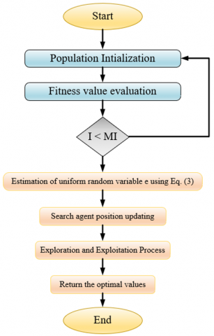
Figure 3. The flowchart of the suggested EPU-CSO
3.1 Parameter optimization using EPU-CSO
The classical CSO is adopted from the circle’s geometrical features. One of the well-known object is a circle that has multiple features especially the centre, tangent line, diameter, and the perimeter. The circle is the curve which is enhanced with the same amount of distance among the middle point and the entire points. The CSO is a robust and simple approach. It produces effective solutions. In order to enhance the accuracy rate EPU-CSO approach is implemented because the conventional CSO takes the uniform random number e in between 0 and 1. This may reduce the correctness of the approach. So, the new EPU-CSO approach estimates the variable e according to the fitness values of the CSO. The calculation of the uniform random variable e is derived in Eq. (3).
e=\frac{b e f}{w o f} (3)
where, bef represents the best fitness found by the conventional CSO algorithm. This is the highest or most optimal solution encountered during the optimization process. Further, wof: Represents the worst fitness in the conventional CSO algorithm. This is the least optimal solution observed in the process.
Significance of the Ratio e in EPU-CSO
•Guiding Parameter Estimation: The ratio e can be used to estimate parameters or adjustments within the EPU-CSO algorithm.
•Range of Search Space Adjustment: If e is close to 1, it indicates that the fitness values are similar, suggesting a potentially narrower range of search space or less need for exploration. Conversely, if e is much less than 1, it indicates a larger spread between the best and worst solutions, which might necessitate a broader search space or more extensive exploration.
•Scaling of Random Variables: The value of e can influence how random variables are scaled. For example, a larger ratio might result in scaling that favors exploration of diverse areas, while a smaller ratio could focus on refining solutions within a smaller region.
•Refinement of Search Process: As the algorithm progresses, the ratio e helps adjust the search strategy. If the fitness values converge (i.e., e approaches 1), the algorithm might shift towards a more refined search or exploitation of promising regions. Conversely, if there is a wide spread, the algorithm may emphasize exploration to find better solutions.
The primary phases of the traditional CSO [30] are as follows. The starting phase of the CSO is the initialization of the attributes. In this phase, the entire dimension of each search member should be equally selected randomly.
The search member's initialization is conducted between the lower ll and the upper ul limit factors of the exploring region. This is given by Eq. (4).
T_s=l l+p \times(u l-l l) (4)
In the above expression, the variable p specifies the arbitrary vector that has a range from 0 to 1.
The next phase is started when the search member position’s updated. Depending on the validated best position Te, the place of the search member Ts is upgraded. This phase is derived in Eq. (5).
T_s=T_e+\left(T_e-T_s\right) \times \tan (\theta) (5)
The importance of the angle \theta in the above expression is very essential for the conventional CSO scheme’s phases of exploration and the exploitation. These are evaluated from Eq. (6) and Eq. (9).
\mathrm{Q}(s, a)=\mathbb{E} s^{\prime}\left[R(s, a)+\gamma \max a^{\prime} Q^{\left(s^{\prime}, a^{\prime}\right)}\right] (6)
\beta=\beta \times r m-\beta (7)
c=\pi-\pi \times\left(\frac{I}{M I}\right)^2 (8)
f=1-0.9 \times\left(\frac{I}{M I}\right)^{0.5} (9)
The arbitrary measure is pointed as r m with the range [0, 1] and the iteration counted is denoted as I. The conventional CSO utilized a constant variable as with a limit [0, 1] which may reduce the accuracy rates. So that in the presented EPU-CSO, the variable is estimated utilizing Eq. (3). And the maximum number of iterations is specified as M. The term \beta in Eq. (7) changes from to 0 when the iteration number gets increased in the process. In addition, the factor c in Eq. (8) changes from -\pi to 0. Further, the measure f in Eq. (9) changes from 1 to 0. In the end, the variable changes from -\pi to 0.
The classical CSA adopts two phases to perform the executions and that is explained as follows.
Case (i) I>(e . M I): This condition is enabled when the angle is \theta=\beta \times r m and it can be provided to increase the exploration phase of the CSO.
Case (ii) I<(e . M I): This condition generates when the overall angle time is \theta=\beta \times r and that can employ to increase the phase of the exploitation.
Algorithm 1 specifies the pseudo-code of the suggested EPU-CSO algorithm and the Figure 3 offers the flowchart of the presented EPU-CSO.
|
Algorithm 1: Recommended EPU-CSO |
|
|
Initialization of the population and the execution parameters |
|
|
Objective function estimation |
|
|
For to I=1 \text{to} M I |
|
|
For to s=1 to N_{p o p} |
|
|
Estimate the uniform random variable utilizing Eq. (3). |
|
|
|
Process the search agent initialization by applying Eq. (4). |
|
|
Position updating of search agent employing Eq. (5). By utilizing the significant factors perform the exploration and exploitation stages. |
|
End |
|
|
End |
|
|
|
Do the iterative iterations to accomplish the better outcomes. |
|
|
Offer the optimal solution. |
|
End |
|
EPU-CSO combines a parameter ratio e to modify the search strategy, therefore affecting the exploration and circular search strategies. This suggested approach uses the ratio e, which influences parameter estimation, search space range, and scaling of random variables, so having a more dynamic adjusting mechanism. It also adjusts the balance dynamically depending on the fitness values noted during the optimization process using the ratio e.
3.2 Trans-ResUnet for segmentation
The image segmentation is conducted by changing an image into a set of pixels which are indicated by the image designated. In the suggested kidney tumor detection approach, the pre-processed picture G_a^{p p} is provided to the segmentation phase which is performed with the support of Trans-ResUnet. This network is the composition of the "Transformer and ResUnet". The transformer [31] approach is managing the problem of deep learning. In this task, the tokenization process is utilized by changing the provided input into a demolished 2D specks collection \left\{G_a^j \in R^{a^2 . D} \mid j=1,2, \ldots J\right\}, here the variable a \times a denoted as the patch size, and the variable M= \frac{J W}{a^2} indicates the image specks amount. Further, the patch embedding is conducted. Here, the patches which are vectorized G_a are linked together with the region of D dimensional embedding by adopting the understandable sequence projection. Eq. (10) formulates the positional information.
G_0=\left[G_a^1 F ; G_a^2 F ; \ldots ; G_a^J F\right]+F_{p a s} (10)
The variable F \in R^{\left(a^2 . D\right) \times E} specifies the "patch embedding projection" and the "position embedding" is denoted as F_{p o s} \in R^{M \times E}.
There are V layers of “Multihead Self-Attention (MSA)” and “Multi-Layer Perceptron (MLP)” in the transformer encoder. Hence, the answer to the layer is expressed by Eq. (11) and Eq. (12):
G_v^{\prime}=M S A\left(L N\left(G_{v-1}\right)\right)+G_{v-1} (11)
G_v=M L P\left(L N\left(G_v^{\prime}\right)\right)+G_v^{\prime} (12)
The attribute LN points to the normalization of the layer and the variable G_v terms the encoded representation of the image.
Figure 4 shows the Trans-Resnet architecture for the segmentation that includes encoding, decoding and attention mechanism. Where the encoding path narrows down the spatial dimensions while extracting features, and the decoding path up samples the feature maps to reconstruct the original image with segmentation information. The attention mechanism helps the model focus on relevant parts of the image, improving its performance.
Because of the attribute lost identities in the deep NN implemented by the minimized weight attribute gradients maximizes the degradation. The ResUnet [32] is the deep U-net that is an encoder-decoder framework for the semantic segmentation. The ResUnet combines the three paths of coding into the framework of encoding-decoding. The ResUnet utilizes the features of both deep residual learning and Unet. The ResUnet framework is the fully CNN with minimal attributes that focuses to attain better functionality. It is the improved version of the conventional U-Net framework. The ResUnet includes a decoding and encoding network and to connect these two networks there is a bridge. The U-net utilizes two 3×3 convolutions. Every convolution has an activation function. When focusing on the ResUnet, these layers are exchanged by the residual block. The TransResUnet framework’s architecture is illustrated.
Figure 4. The architecture of the Trans-ResUnet for the image segmentation in the suggested kidney tumor detection approach
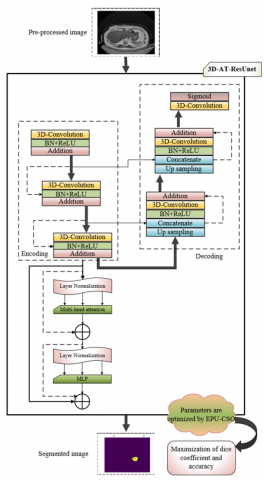
3.3 Suggested 3D-AT-ResUnet for segmentation
The Trans-ResUnet is a very compatible and robust approach. This approach is very efficient for the medical image segmentation. However, the network has high computational requirements and utilizes more amounts of parameters. So, the suggested kidney tumor detection mechanism presented the 3D-ATR mechanism for the effective segmentation approach. Here, the pre-processed image G_a^{p p} is subjected as an input. This new mechanism executes the images in an “end-to-end” way and performs the 3D evaluation on the both decoder and encoder sides. This approach employs the 3D convolution for the effective functionality and successive outcomes. The 3D-ATR approach overcomes the complexities of the conventional approaches. The transformer-ResUnet includes several attributes such as hidden neurons, step per epoch, and the number of epochs. The high amount of these attributes raises the network complexities and leads to overfitting. So, that these attributes are optimally tuned in this suggested mechanisms. For that purpose, the developed EPU-CSO is utilized. The objective function of this task is given by Eq. (13).
o b_1=\underset{\left\{hn^{3 D-A T R}, e p^{3 D-A T R}, s e^{3 D-A T R}\right\}}{\arg \max }[D c+A c] (13)
Here, the steps per epochs in 3D-AT-ResUnet are given as s e^{3 D-A T R} and the hidden neuron counts in 3D-AT-ResUnet are specified as h n^{3 D-A T R}, and the number of epochs in 3D-AT-ResUnet is denoted as e p^{3 D-A T R}. Moreover, the steps per epoch in 3D-AT-ResUnet vary from 300 to 1000 and the hidden neuron counts in 3D-AT-ResUnet are changed from 5 to 255. Also, the “number of epochs” in 3D-AT-ResUnet falls from 5 to 50. The variable D c indicates the “dice coefficient” which is the overlap among the segmented and masked pictures. Besides, the variable A c specifies the accuracy which finds the relationship among the original and processed images. The formulations of these two variables are given in Eq. (14) and Eq. (15):
D c\left(G_a, G_a^{ {seg }}\right)=\frac{2\left(G_a \cap G_a^{\text {seg }}\right)}{G_a+G_a^{ {seg }}} (14)
A c=\frac{s a+n t}{s a+n t+h i+y a} (15)
where, the variable G_a^{s e g} indicates the segmented image, and the factor ya point to the “false negative”. The term hi denotes the “false positive” and the variable nt refers to the “true negative”. Also, the factor sa indicates the “true positive”. In the end, the effective segmented images G_a^{s e g} are attained from the suggested 3D-AT-ResUnet framework. The 3D-AT-ResUnet appears in Figure 5, showcasing parameter tuning. The visual displays the 3D AT-Res U-Net architecture, which is a specialized deep learning model created for the purpose of segmenting medical images. This model is an enhanced version of the conventional U-Net design, which integrates attention mechanisms and residual connections to enhance performance.
Figure 5. The framework of the 3D-AT-ResUnet mechanism for the segmentation approach with parameter optimization
4.1 Residual Attention Network (RAN)
The RAN [33] is generated by ordering various attention sections. Here, the segmented image G_a^{s e g} is given as an input. In RAN, every attention sector is partitioned into two branches. They are named as “trunk branches and mask branches”. With the support of the trunk branch, the attribute processing is conducted to any of the successive frameworks. In this RAN, the fundamental components to creating the attention sector are inception, “ResNeXt” and the residual unit. Assume the answer of the trunk branch {Tr}\left(G_a^{s e g}\right) with the provided input G_a^{s e g}; the “bottom-up” and “top-down” strategies are utilized by the mask branch in order to understand the similar dimension mask Ma(G_a^seg ) that finely weighs the resultant attributes {Tr}\left(G_a^{s e g}\right). The “bottom-up” and “top-down” strategies copy the approaches of feedback attention and the fast feed-forward. The resultant mask is applied as the control gates for the trunk branch’s neurons same as the network of highways. Eq. (16) formulates the module of attention A.
A_{j, d}\left(G_a^{ {seg }}\right)=M a_{j, d}\left(G_a^{ {seg }}\right) * T r_{j, d}\left(G_a^{\ {seg }}\right) (16)
where, the variable j limits over the entire spatial places d∈{1,...,D} and the attribute points are the channel index.
In the attention sections, the attention masks perform like the attribute selector while processing the forward inference, and also perform like a gradient update filter while performing the backpropagation. When considering the soft mask branch, the input attribute of the mask gradient is derived in Eq. (17).
\frac{\partial M a\left(G_a^{{seg}}, \theta\right) {Tr}\left(G_a^{\operatorname{seg}}, \varphi\right)}{\partial \varphi}=M a\left(G_a^{{seg}}, \theta\right) \frac{\partial {Tr}\left(G_a^{{seg}}, \varphi\right)}{\partial \varphi} (17)
where, the attributes of the mask branch are denoted as θ and the attributes of the trunk branch are pointed as φ.
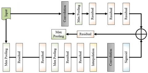
The framework of the RAN method is illustrated in Figure 6. The RAN adheres to a comparable framework as the conventional U-Net, comprising an encoding path that collects characteristics and a decoding path that reconstructs the picture by using segmentation information. The main distinction is in the incorporation of residual connections, which effectively tackle the issue of vanishing gradient and enhance the model's capacity to acquire profound features.
Figure 6. The framework of RAN for the recommended kidney tumor detection mechanism
4.2 Proposed MT-RAN for detection
Designing the contextual data of a picture is important for generating the correctness of the tumor identification in the segmented pictures. Hence, the multi-scale transformer network [34] is presented in the designed work. Here, the segmented image G_a^{ {seg }} is provided as an input. For the provided attribute map G_a^{{seg }}(a=1,2) \in R^{I \times X \times D} is partitioned into various token sequences with the similar width and lengths O^a(a=1,2) \in R^{M \times D}, combine O^1 and O^2 into the variable O, and further the input O into the network of the transformer. The primary transformer components are "Multihead Cross-Attention (MCA)", MLP, and MSA.
Considering that the layer’s input sequence s is O_{s-1} and O_s^{f^{\prime}} attained via the “preNorm” sector in Eq. (18).
O_s^{f^{\prime}}=P N\left(O_{s-1}\right) (18)
where, the MSA sector’s input is denoted as O_s^{f^{\prime}} and the term PN referred to as the “PreNorm”. The expression of the MSA is given in Eq. (19) and Eq. (20).
{MSA}\left(O_{s-1}\right)={concat}\left(B_1, \ldots, B_i\right) X^P (19)
B_j=\alpha\left(\frac{\left(O_s^{f^{\prime}} X_j^r\right)\left(O_s^{f^{\prime}} X_j^l\right)^T}{\sqrt{e}}\right)\left(O_s^{f^{\prime}} X_j^w\right) (20)
The connection operation is denoted as concat and the softmax function is specified as \alpha. The arbitrary layer is indicated as j. The attributes X_j^r, X_j^l and X_j^\omega \in R^{D \times e}, X^P \in R^{i e \times D} are denoted as the matrix of learnable parameters. The attention head is represented as B and the attention head is pointed as i. Also, the number of layers is indicated as s-1 and the variable e specifies the channel dimension. The estimation of MSA is derived in Eq. (21).
O_s^{f^{\prime \prime}}=M S A\left(P N\left(O_{s-1}\right)\right)+O_{s-1} (21)
In common, the transformer encoder’s estimation operation is formulated in Eq. (22).
O_e^f=M L P\left(P N\left(O_s^{f^{\prime}}\right)\right)+O_s^{f^{\prime \prime}} (22)
The MSA section’s solution is denoted as O_s^{f^{\prime \prime}} and the MLP section’s solution is referred as O_s^f .
To better understand the data interaction of the images, the MSA is exchanged with the MCA. Considering the variable O_s as the input sequence s and the corresponding derivation of the MCA is derived in Eq. (23) and Eq. (24).
M C A\left(O_{s-1}^a, O_s^{f, a}\right)={concat}\left(B_1, \ldots, B_i\right) X^P (23)
B_j=\alpha\left(\frac{\left(P N\left(O_{s-1}^a\right) X_j^r\right)\left(O_s^{f, a} X_j^l\right)^T}{\sqrt{e}}\right)\left(O_s^{f, a} X_j^w\right) (24)
The MCA’s calculation operation is formulated in Eq. (25):
O_{s+1}^{e, a^{\prime}}=M C A\left(P N\left(O_{s-1}^a\right), O_s^{f, a}\right)+O_{s-1}^a (25)
In common, the calculation operation of the transformer is formulated in Eq. (26).
O_{s+1}^{e, a}=M L P\left(P N\left(O_{s+1}^{e, a^{\prime}}\right)\right)+O_{s+1}^{e, a^{\prime}} (26)
The solution of the MLP and MCA section are denoted as O_{s+1}^{e, a} and O_{s+1}^{e, a,} and accordingly.
Multi-scale transformer: It is motivated by the “Pyramid Pooling Module (PPM)”. The data at various measures in the attribute map is drawn out by developing the four transformers with distinct measures. The four attribute maps of distinct sizes G_1^{ {seg }}, G_2^{ {seg }}, G_3^{ {seg }} and G_4^{\ {seg }} and are attained by down sampling and convolutions of variables G_1^{ {seg }}. Enter the variables into respective transformers which have the distinct measures for performing the feature extraction and also for attaining the variables G_1^{ {new }}, G_2^{ {new }}, G_3^{ {new }} and G_4^{ {new }}. The attribute maps with a similar number of channels, width, and heights as G_1^{ {new }} are attained by distinct up sampling and convolutions of the variables G_2^{ {new }}, G_3^{ {new }} and G_4^{ {new }} accordingly. In the end, the four attribute maps are linked by the addition. So, the Multiscale transformer MST is formulated in Eq. (27).
{MST}\left(G_a^{s e g}\right)=\sum_{a=1}^4\left(u c_a\left(\operatorname{tr}_a\left(d c_a\left(G_a^{s e g}\right)\right)\right)\right) (27)
where, the variable t r_a indicates the transformer section and the factor u c_a specifies the convolution and up sampling. Moreover, the factor d c_a denotes the convolution and down sampling.
Figure 7. The functional diagram of the suggested MT-RAN for the kidney tumor detection mechanism
MT-RAN: The conventional RAN can perform well in the medical image applications. It produces better outcomes. However, it is very hard to train and develop. It also has the overfitting issues. On the other side, the traditional multi-scale transformer reduces the computation time and the memory utilization. But this network also has several problems like unexpected outcomes when the utilization of a high amount of inputs. So, to achieve the effective classification of the suggested kidney tumor detection approach, the MT-RAN mechanism is adopted. Here, the advantages of these two networks are integrated and help to solve the conventional network issues. Finally, the better classification outcomes are attained with the support of recommended MT-RAN approach for the kidney tumor. Figure 7 exhibits the diagram of the suggested MT-RAN technique for the detection mechanism of kidney tumors. The model for medical imaging segmentation is created by including U-Net, residual connections, and transformer blocks, which results in a very effective combination of techniques. The transformer block is an essential element that enables the model to effectively capture distant relationships within the input image. Residual connections and skip connections enhance the stability and performance of training.
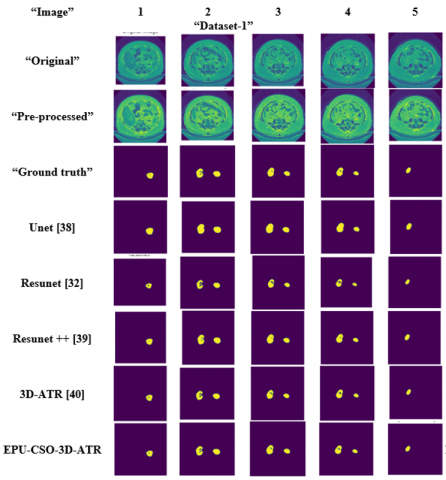
4.3 Image results
The suggested kidney tumor detection approach is successfully executed and the resultant images are given in Figure 8 for two datasets.
The Figure 8 illustrates 5 sample images from Dataset-1 and Dataset-2, showcasing a comparison between the original image, pre-processed image, and ground truth. The end results of several models, including the proposed approach, are also presented.
Figure 8. The resultant images of the designed kidney tumor detection approach for both datasets
5.1 Simulation setup
Python platform has been used to process the recommended kidney tumor detection mechanism and remarkable outcomes were achieved. The proposed kidney tumour detection approach employs 10 different combinations of the parameters at each generation i.e., 10 populations and each solution in these populations is characterized by 3 parameters or 3 chromosome lengths for segmentation, classification and overall architecture. Moreover, the maximum iteration count of the recommended kidney tumor detection framework was 50. Some of the traditional optimization algorithms like Tuna Swarm Optimization (TSO) [35], Coyote Optimization Algorithm (COA) [36], Fire Hawk Optimizer (FHO) [37], and CSO [28] are utilized for the evaluation process. In addition, several segmentations approach like Unet [38], ResUnet [32], ResUnet++[39], and 3D-ATR [40] were adopted. Also, the detection mechanisms such as CNN [41], LSTM [42], Mobilenet [43], and Resnet [44] were employed for the estimation of the recommended kidney tumor detection mechanism.
5.2 Evaluation metrics
The suggested kidney tumor detection mechanism utilized several performance metrics for the evaluation. These are given as follows.
Dice coefficient: Measures the similarity between two sets, typically the predicted and ground truth segmentations. It ranges from 0 (no overlap) to 1 (perfect overlap). It is formulated in Eq. (14). In medical imaging, the Dice coefficient determines how closely the ground truth region identified by an expert overlaps the expected tumor region.
Accuracy: The proportion of correctly classified pixels (or regions) out of all the pixels. It is formulated in Eq. (15).
In image classification or segmentation, it indicates the algorithm's accuracy in accurately identifying both positive (e.g., tumor) and negative (e.g., non-tumor) pixels.
Jaccard coefficient: It is employed to validate the percentage of the overlap among the gatherings.
J c\left(G_a, G_a^{s e g}\right)=\frac{\left|G_a \cap G_a^{s e g}\right|}{\left|G_a \cup G_a^{s e g}\right|} (28)
where, Ga represents original image, and G_a^{s e g} is segmented image. Jaccard coefficient is used to evaluate how well the algorithm detects the correct area of an object like a tumor by computing the overlap between the predicted and actual regions.
Precision: It is the description of the arbitrary errors and estimates the variability of the statistics.
P=\frac{s a}{s a+n t} (29)
It measures how accurate the model is in predicting true positives without falsely predicting non-tumor regions as tumors.
NPV: It estimates the rate of true negative estimations concerning overall negative estimations.
N P V=\frac{h i}{h i+y a} (30)
NPV in medical imaging refers to the probability that areas identified as non-tumor are indeed non-tumor, hence offering confidence in the negatives.
FPR: It is the factor to estimate the probability of the correctness.
F P R=\frac{n t}{n t+h i} (31)
FPR analyzes the rate at which the model mistakenly labels non-tumor areas as tumors, therefore causing unwarranted treatments.
F1-score: It integrates the scores of the precision and recall.
F 1-Score =\frac{2 \times s a}{2 \times s a+n t+y a} (32)
The F1-score gives an overall sense of the balance between precision (accuracy of positive predictions) and recall (sensitivity).
FDR: It is utilized to correct the various comparisons.
F D R=\frac{n t}{n t+s d} (33)
FDR assesses how often the model incorrectly predicts a positive (e.g., a tumor) when it’s actually not, indicating potential over-diagnosis.
Sensitivity: It is the likelihood of a positive test outcome.
Sen =\frac{s a}{s a+y d} (34)
Sensitivity measures how effectively the model detects all actual positive cases (e.g., all tumors), critical for ensuring that important anomalies are not missed.
Specificity: It evaluates how well the experiment detects the true negative.
s p e c=\frac{h i}{h i+n t} (35)
Specificity measures how well the model identifies non-tumor areas, important to avoid false positives that could lead to unnecessary treatments.
MCC: It is the correlation factor among the monitored and estimated classifications.
M C C=\frac{s a \times h i-n t \times y a}{\sqrt{(y a+s a)(y a+h i)(s a+n t)(h i+n t)}} (36)
MCC is useful for binary classification problems (e.g., tumor vs. non-tumor) and is a more reliable metric when class sizes are imbalanced. For all above evaluation metrics, we have used the folowing terms for notation: Ga – original image, G_s^{\arg } – segmented image, sa – true positives, nt- false positives, ya – false negatives, and hi – true positives.
5.3 Confusion matrix estimation of the recommended kidney tumor detection approach
The recommended kidney tumor detection mechanism is processed with the confusion matrix to estimate the accuracy of the network for the two datasets. This is presented in Figure 9. The accuracy of the suggested kidney tumor detection approach is enriched by 96.18% when considering the second data resource in Figure 9(b) (The presented accuracy scores for Dataset 1 and Dataset 2, is 95.38% and 96.18%, respectively, provides additional evidence that supports this observation). From this, it is highlighted that the designed kidney tumor identification mechanism has better efficacy.
Figure 9. The confusion matrix evaluation of the recommended kidney tumor detection framework concerning, (a) Dataset 1, and (b) Dataset 2
5.4 ROC investigation of the suggested kidney tumor detection mechanism over various classifiers
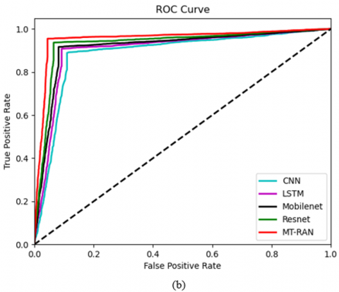
Figure 10 shows the ROC investigation of the developed kidney tumor detection framework against various classifiers for the two data resources. The ROC is validated based on the “true and false” positive rates. For the first data resource in Figure 10(a), the ROC of the suggested kidney tumor mechanism is advanced by 45% of CNN, 46% of LSTM, 50% of Mobilenet, and 53% of Resnet accordingly when taking the “false positive rate” value is 0.6. Hence, the suggested kidney tumor detection approach has outperformed other classifiers.
Figure 10. The ROC calculation of the suggested kidney tumor identification framework over various conventional classifiers concerning, (a) Dataset 1, and (b) Dataset 2
5.5 Convergence estimation of the designed EPU-CSO algorithm over diverse conventional algorithms
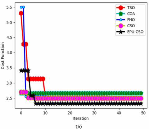
The designed EPU-CSO algorithm is validated with the convergence measure against diverse traditional algorithms and provided in Figure 11 for the two data sources. The amount of iteration is employed for this process. For the second data source in Figure 11 (b), the convergence of the suggested EPU-CSO scheme has maximized by 91% of TSO, 91% of COA, 92% of FHO, and 92.3% of CSO appropriately when the number of iterations is 30. The outcomes highlight that the recommended EPU-CSO has better convergence rates.
Figure 11. The convergence investigation of the suggested EPU-CSO algorithm over diverse optimization algorithms regarding, (a) Dataset 1, and (b) Dataset 2
5.6 Statistical report of the improved EPU-CSO algorithm over multiple optimization algorithms
Table 2 offers the surprising statistical outcomes of the designed EPU-CSO scheme against various conventional algorithms for the two datasets. The suggested EPU-CSO has improved by 30% of TSO, 16% of COA, 14% of FHO, and 14.2% of CSO correspondingly when considering the best factor in the first dataset. From this, it is confirmed that the developed EPU-CSO has higher functionalities. Looking at best, mean, median values, EPU-CSO shows the best performance on both datasets; this indicates that it is often able to identify better solutions on average and also performs regularly well. Although CSO is not the best performer in all measures, typically it shows a balance of strong performance with low variability in findings on Dataset-1.
Table 2. The statistical validation of the designed EPU-CSO algorithm over various optimization algorithms for two datasets
|
TERMS |
TSO [35] |
COA [36] |
FHO [37] |
CSO [28] |
EPU-CSO |
|
Dataset-1 |
|||||
|
Best |
2.950357378 |
4.965917477 |
4.833117508 |
3.699706316 |
4.206566095 |
|
Worst |
2.539995678 |
2.500192071 |
2.490755428 |
2.63356704 |
2.385363785 |
|
Mean |
2.632307251 |
2.807067702 |
2.822918936 |
2.677409884 |
2.578881774 |
|
Median |
2.539995678 |
2.689594334 |
2.645897047 |
2.63356704 |
2.385363785 |
|
Standard Deviation |
0.159728472 |
0.526337456 |
0.540768089 |
0.183001885 |
0.459387195 |
|
Dataset-2 |
|||||
|
Best |
5.302505324 |
2.816151841 |
5.498436454 |
2.705981719 |
3.409528112 |
|
Worst |
2.494961518 |
2.347863549 |
2.47527388 |
2.491229916 |
2.320258137 |
|
Mean |
2.721462302 |
2.653311347 |
2.610263611 |
2.505486431 |
2.418071711 |
|
Median |
2.512099355 |
2.607189457 |
2.47527388 |
2.491229916 |
2.320258137 |
|
Standard Deviation |
0.540105167 |
0.131246540 |
0.590302462 |
0.050943085 |
0.296985703 |
5.7 Functionality validation of the suggested segmentation approach over diverse algorithms and segmentation methods
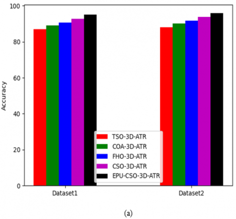
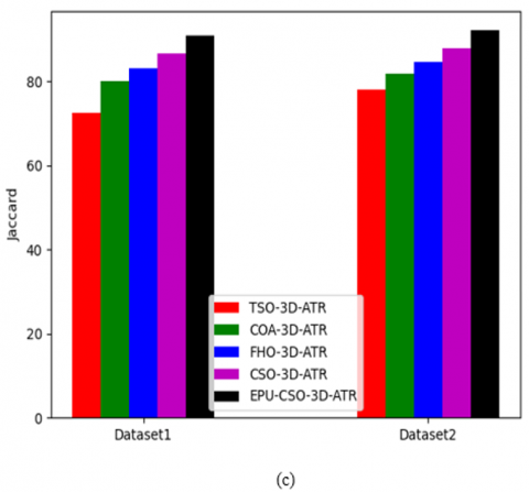
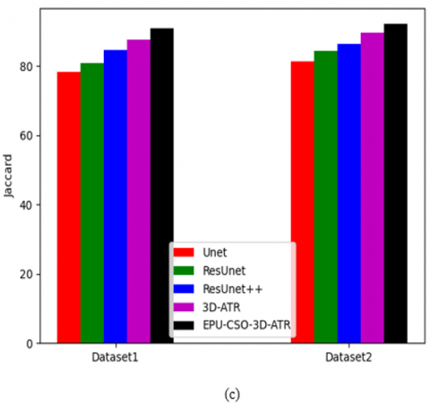
The functionality of the recommended 3D-AT-ResUnet-assisted segmentation task is estimated for the two datasets against various algorithms and segmentation approaches and demonstrated in Figure 12 and Figure 13. When considering the dice coefficient for the first data source in Figure 13 (b), the segmentation process of the recommended kidney tumor detection has enhanced by 85% of Unet, 88% of ResUnet, 91% of ResUnet++, and 93% of 3D-ATR correspondingly. This shows that the suggested 3D-AT-ResUnet-assisted segmentation task in developed kidney tumor detection has effective solutions.
Figure 12. The functionality validation of the designed segmentation process in the kidney tumor detection framework over various optimization algorithms regarding, (a) Accuracy, (b) Dice coefficient, and (c) Jaccard
Figure 13. The functionality estimation of the recommended segmentation process in the kidney tumor detection framework over various segmentation approaches regarding, (a) Accuracy, (b) Dice coefficient, and (c) Jaccard
5.8 Comparative estimation of the recommended kidney tumor detection mechanism over multiple algorithms and classifiers
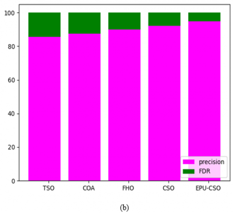
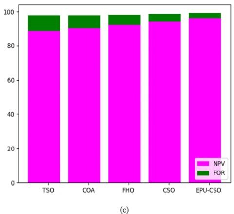
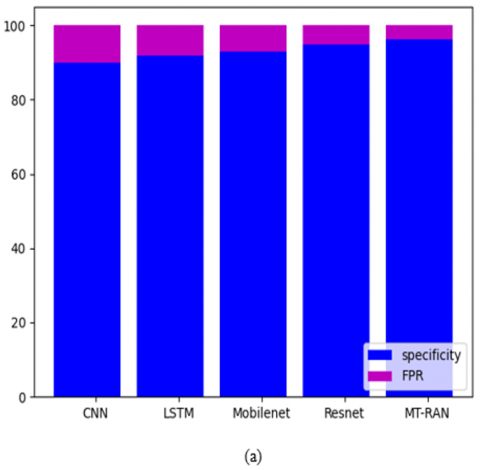
The comparative evaluation of the recommended kidney tumor detection framework over distinct algorithms and classifiers is presented in Figures 14-17 for the two datasets. Several evaluation metrics are utilized to estimate the functionality of the approach. From Figure 14(a), the specificity of the suggested kidney tumor detection approach is enriched by 85% of TSO, 85.5% of COA, 86% of FHO, and 86.5% of CSO appropriately for the first data source over FPR. Thus, the recommended kidney tumor detection task has better functionalities against the pre-existing methodologies.
Figure 14. The comparative research of the designed kidney tumor detection framework over various conventional algorithms for the first data source concerning (a) Sensitivity Vs FPR, (b) Precision Vs FDR, and (c) NPV Vs FOR
Figure 15. The comparative research of the suggested kidney tumor detection framework over various conventional classifiers for the first data source concerning (a) Sensitivity Vs FPR, (b) Precision Vs FDR, and (c) NPV Vs FOR
Figure 16. The comparative research of the suggested kidney tumor detection framework over various conventional algorithms for the second data source concerning (a) Sensitivity Vs FPR, (b) Precision Vs FDR, and (c) NPV Vs FOR
Figure 17. The comparative research of the suggested kidney tumor detection framework over various conventional classifiers for the second data source concerning (a) Sensitivity Vs FPR, (b) Precision Vs FDR, and (c) NPV Vs FOR
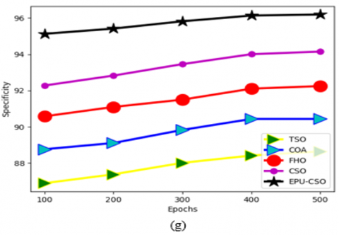
5.9 Performance evaluation of the suggested kidney tumor detection approach over various algorithms and classifiers
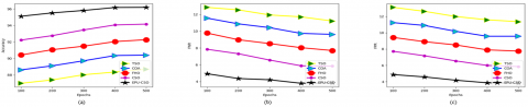
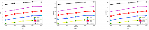
Figures 18-21 illustrate the performance investigation of the recommended kidney failure detection strategy against distinct algorithms and classifiers for the two data resources. By considering the epoch values and some of the performance factors, this operation is performed. For the second data source in Figure 20(a), when the epoch value is 300, the accuracy of the suggested kidney tumor detection mechanism is maximized by 70.8% of CNN, 70.4% of LSTM, 69.3% of Mobilenet and 68.9% of Resnet appropriately. Thus, the suggested kidney tumor detection approach has enriched performance rates against other classical methodologies.
Figure 18. The performance calculation of the suggested kidney tumor identification framework over various conventional algorithms for the first data source concerning, (a) Accuracy, (b) FNR, (c) FPR, (d) NPV, (e) Precision, (f) Sensitivity, and (g) Specificity
Figure 19. The performance calculation of the suggested kidney tumor detection framework over various conventional classifiers for the first data source concerning, (a) Accuracy, (b) FNR, (c) FPR, (d) NPV, (e) Precision, (f) Sensitivity, and (g) Specificity
Figure 20. The performance calculation of the suggested kidney tumor detection framework over various conventional algorithms for the second data source concerning, (a) Accuracy, (b) FNR, (c) FPR, (d) NPV, (e) Precision, (f) Sensitivity, and (c) Specificity
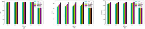
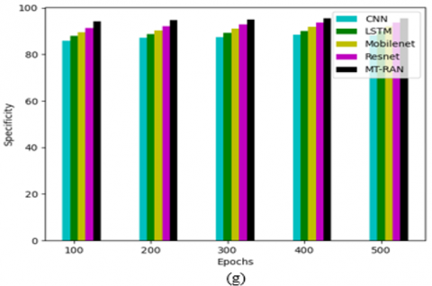
Figure 21. The performance calculation of the suggested kidney tumor detection framework over various conventional classifiers for the second data source concerning, (a) Accuracy, (b) FNR, (c) FPR, (d) NPV, (e) Precision, (f) Sensitivity, and (c) Specificity
5.10 Overall comparative evaluation of the recommended kidney tumor detection approach over various conventional algorithms and classifiers
Table 3 and Table 4 offer the overall comparative validation of the recommended kidney tumor detection mechanism over various algorithms and classifiers for two datasets. The specificity of the recommended kidney tumor detection approach is enhanced by 7.9% of TSO, 6% of COA, 4.1% of FHO, and 2.4% of CSO correspondingly when taking the first dataset in Table 3. Hence, the outcomes explained that the suggested kidney tumor detection mechanism has better functionalities.
Table 3. The overall comparative estimation of the designed kidney tumor identification strategy over diverse traditional algorithms for two datasets
|
TERMS |
TSO [35] |
COA [36] |
FHO [37] |
CSO [28] |
EPU-CSO |
|
Dataset 1 |
|||||
|
Accuracy |
87.82978723 |
89.5106383 |
91.27659574 |
93.10638298 |
95.38297872 |
|
Recall |
88.05309735 |
89.46902655 |
91.0619469 |
93.18584071 |
95.39823009 |
|
Specificity |
87.75910364 |
89.52380952 |
91.34453782 |
93.08123249 |
95.37815126 |
|
Precision |
69.48324022 |
72.99638989 |
76.9058296 |
81 |
86.72566372 |
|
FPR |
12.24089636 |
10.47619048 |
8.655462185 |
6.918767507 |
4.621848739 |
|
FNR |
11.94690265 |
10.53097345 |
8.938053097 |
6.814159292 |
4.601769912 |
|
NPV |
95.86903305 |
96.41025641 |
96.99583581 |
97.73529412 |
98.49580561 |
|
FDR |
30.51675978 |
27.00361011 |
23.0941704 |
19 |
13.27433628 |
|
F1-Score |
77.67369243 |
80.39761431 |
83.38735818 |
86.66666667 |
90.85545723 |
|
MCC |
0.703882069 |
0.740447691 |
0.780383012 |
0.82415189 |
0.879550828 |
|
Dataset 2 |
|||||
|
Accuracy |
88.70703764 |
90.4091653 |
92.27495908 |
94.15711948 |
96.18657938 |
|
Recall |
88.78787879 |
90.37878788 |
92.31060606 |
94.16666667 |
96.17424242 |
|
Specificity |
88.64553314 |
90.43227666 |
92.24783862 |
94.14985591 |
96.19596542 |
|
Precision |
85.60993426 |
87.78513613 |
90.05912786 |
92.45072518 |
95.0580307 |
|
FPR |
11.35446686 |
9.567723343 |
7.752161383 |
5.850144092 |
3.804034582 |
|
FNR |
11.21212121 |
9.621212121 |
7.689393939 |
5.833333333 |
3.825757576 |
|
NPV |
91.22182681 |
92.51179245 |
94.03642773 |
95.49839228 |
97.06309974 |
|
FDR |
14.39006574 |
12.21486387 |
9.940872136 |
7.549274823 |
4.9419693 |
|
F1-Score |
87.16995165 |
89.06308324 |
91.17096895 |
93.30080691 |
95.61287893 |
|
MCC |
0.771319999 |
0.805535864 |
0.843266825 |
0.881326286 |
0.922455851 |
Table 4. The overall comparative estimation of the designed kidney tumor identification strategy over diverse traditional classifiers for two datasets
|
TERMS |
CNN [41] |
LSTM [42] |
Mobilenet [43] |
Resnet [44] |
MT-RAN |
|
Dataset 1 |
|||||
|
Accuracy |
88.25531915 |
90.04255319 |
91.9787234 |
93.72340426 |
95.38297872 |
|
Recall |
88.14159292 |
90.08849558 |
91.85840708 |
93.80530973 |
95.39823009 |
|
Specificity |
88.29131653 |
90.0280112 |
92.01680672 |
93.69747899 |
95.37815126 |
|
Precision |
70.43847242 |
74.09024745 |
78.45804989 |
82.49027237 |
86.72566372 |
|
FPR |
11.70868347 |
9.971988796 |
7.983193277 |
6.302521008 |
4.621848739 |
|
FNR |
11.85840708 |
9.911504425 |
8.14159292 |
6.194690265 |
4.601769912 |
|
NPV |
95.92209373 |
96.6325917 |
97.27568848 |
97.95021962 |
98.49580561 |
|
FDR |
29.56152758 |
25.90975255 |
21.54195011 |
17.50972763 |
13.27433628 |
|
F1-Score |
78.30188679 |
81.30990415 |
84.631064 |
87.78467909 |
90.85545723 |
|
MCC |
0.71218896 |
0.752732809 |
0.797005866 |
0.838973622 |
0.879550828 |
|
Dataset 2 |
|||||
|
Accuracy |
90.11456628 |
91.94762684 |
92.96235679 |
94.76268412 |
96.18657938 |
|
Recall |
90.22727273 |
91.81818182 |
92.99242424 |
94.77272727 |
96.17424242 |
|
Specificity |
90.02881844 |
92.04610951 |
92.93948127 |
94.75504323 |
96.19596542 |
|
Precision |
87.31671554 |
89.77777778 |
90.92592593 |
93.21907601 |
95.0580307 |
|
FPR |
9.971181556 |
7.95389049 |
7.060518732 |
5.244956772 |
3.804034582 |
|
FNR |
9.772727273 |
8.181818182 |
7.007575758 |
5.227272727 |
3.825757576 |
|
NPV |
92.37137788 |
93.66568915 |
94.57478006 |
95.97197898 |
97.06309974 |
|
FDR |
12.68328446 |
10.22222222 |
9.074074074 |
6.780923994 |
4.9419693 |
|
F1-Score |
88.74813711 |
90.78651685 |
91.94756554 |
93.98948159 |
95.61287893 |
|
MCC |
0.79971588 |
0.836536145 |
0.857160346 |
0.893592541 |
0.922455851 |
A novel kidney tumor detection mechanism has been implemented using deep learning technology. In this task, the essential images were accumulated and subjected to the pre-processing stage. The pre-processing step involved two mechanisms such as weighted mean histogram equalization and the contrast enhancement. Further, the pre-processed images were fed into the segmentation task where the 3D-ATR was adopted. The attributes which were existed in this network were optimized with the aid of the designed EPU-CSO scheme. Besides, the segmented images were offered for the classification of kidney tumor stage where the MT-RAN was adopted. The recommended kidney tumor detection mechanism attained a higher efficiency rate than the traditional mechanisms in various research estimations. When considering the first data source epoch value as 200, the accuracy of the suggested kidney tumor detection approach is maximized by 56.85% of TSO, 55.95% of COA, 55% of FHO, and 54.1% of CSO correspondingly. Hence the suggested kidney tumor mechanism performed better than the traditional approaches. In future, the recommended kidney tumor detection mechanism will be deployed with the hybrid heuristic algorithm to enhance the accuracy rates. The implemented kidney tumor classification system offered highly accurate outcomes. However, while processing large-scale datasets, the quality of the outcome is minimized. Hence, in future work, more effective techniques will be integrated into the suggested work for improving the quality of the outcome. Moreover, the designed system has not classified the cancer subtypes. Therefore, in future work, the designed kidney tumor classification system will be improved for classifying the tumor subtypes for offering valuable data for further experiments. This will also support medical experts in making better treatment decisions.
[1] Chen, X., Summers, R., Yao, J. (2010). FEM based 3D tumor growth prediction for kidney tumor. In Medical Imaging and Augmented Reality: 5th International Workshop, MIAR 2010, Beijing, China, pp. 159-168. https://doi.org/10.1109/TBME.2010.2089522
[2] Chen, X., Summers, R.M., Yao, J. (2012). Kidney tumor growth prediction by coupling reaction–diffusion and biomechanical model. IEEE Transactions on Biomedical Engineering, 60(1): 169-173. https://doi.org/10.1109/TBME.2012.2222027
[3] Yu, Q., Shi, Y., Sun, J., Gao, Y., Zhu, J., Dai, Y. (2019). Crossbar-net: A novel convolutional neural network for kidney tumor segmentation in CT images. IEEE Transactions on Image Processing, 28(8): 4060-4074. https://doi.org/10.1109/TIP.2019.2905537
[4] Causey, J., Stubblefield, J., Qualls, J., Fowler, J., Cai, L., Walker, K., Guan, Y.F., Huang, X. (2021). An ensemble of U-Net models for kidney tumor segmentation with CT images. IEEE/ACM Transactions on Computational Biology and Bioinformatics, 19(3): 1387-1392. https://doi.org/10.1109/TCBB.2021.3085608
[5] Deng, S.P., Cao, S., Huang, D.S., Wang, Y.P. (2016). Identifying stages of kidney renal cell carcinoma by combining gene expression and DNA methylation data. IEEE/ACM Transactions on Computational Biology and Bioinformatics, 14(5): 1147-1153. https://doi.org/10.1109/TCBB.2016.2607717
[6] Gloger, O., Tonnies, K.D., Liebscher, V., Kugelmann, B., Laqua, R., Volzke, H. (2011). Prior shape level set segmentation on multistep generated probability maps of MR datasets for fully automatic kidney parenchyma volumetry. IEEE Transactions on Medical Imaging, 31(2): 312-325. https://doi.org/10.1109/TMI.2011.2168609
[7] Chen, G., Ding, C., Li, Y., Hu, X., Li, X., Ren, L. (2020). Prediction of chronic kidney disease using adaptive hybridized deep convolutional neural network on the internet of medical things platform. IEEE Access, 8: 100497-100508. https://doi.org/10.1109/ACCESS.2020.2995310
[8] Abdullah, S., Jaddi, N.S. (2020). Dual kidney-inspired algorithm for water quality prediction and cancer detection. IEEE Access, 8: 109807-109820. https://doi.org/10.1109/ACCEfSS.2020.3001685
[9] Liu, D., Shao, J., Liu, H., Cheng, W. (2021). Design on early warning system for renal cancer recurrence based on CNN-based Internet of Things. IEEE Access, 10: 34835-34845. https://doi.org/10.1109/ACCESS.2021.3114227
[10] Suomi, V., Jaros, J., Treeby, B., Cleveland, R.O. (2017). Full modeling of high-intensity focused ultrasound and thermal heating in the kidney using realistic patient models. IEEE Transactions on Biomedical Engineering, 65(5): 969-979. https://doi.org/10.1109/TBME.2017.2732684
[11] Dillenseger, J.L., Guillaume, H., Patard, J.J. (2006). Spherical harmonics based intrasubject 3-D kidney modeling/registration technique applied on partial information. IEEE Transactions on Biomedical Engineering, 53(11): 2185-2193. https://doi.org/10.1109/TBME.2006.883653
[12] Rashed-Al-Mahfuz, M., Haque, A., Azad, A., Alyami, S.A., Quinn, J.M., Moni, M.A. (2021). Clinically applicable machine learning approaches to identify attributes of chronic kidney disease (CKD) for use in low-cost diagnostic screening. IEEE Journal of Translational Engineering in Health and Medicine, 9: 1-11. https://doi.org/10.1109/JTEHM.2021.3073629
[13] Kronenberg, A., Gauny, S., Grossi, G., Dan, C., Grygoryev, D., Turker, M. (2014). Genotoxicity of charged particles of importance in space flight using murine kidney epithelial cells. Journal of Radiation Research, 55(suppl_1): i77-i78. https://doi.org/10.1093/jrr/rrt191
[14] Skounakis, E., Banitsas, K., Badii, A., Tzoulakis, S., Maravelakis, E., Konstantaras, A. (2013). ATD: A multiplatform for semiautomatic 3-D detection of kidneys and their pathology in real time. IEEE Transactions on Human-Machine Systems, 44(1): 146-153. https://doi.org/10.1109/THMS.2013.2290011
[15] Saleeb, D.A., Helmy, R.M., Areed, N.F., Marey, M., Almustafa, K.M., Elkorany, A.S. (2022). Detection of kidney cancer using circularly polarized patch antenna array. IEEE Access, 10: 78102-78113. https://doi.org/10.1109/ACCESS.2022.3192555
[16] Hussain, M.A., Hamarneh, G., Garbi, R. (2021). Cascaded regression neural nets for kidney localization and segmentation-free volume estimation. IEEE Transactions on Medical Imaging, 40(6): 1555-1567. https://doi.org/10.1109/TMI.2021.3060465
[17] Uhm, K.H., Jung, S.W., Choi, M.H., Hong, S.H., Ko, S.J. (2022). A unified multi-phase CT synthesis and classification framework for kidney cancer diagnosis with incomplete data. IEEE Journal of Biomedical and Health Informatics, 26(12): 6093-6104. https://doi.org/10.1109/JBHI.2022.3219123
[18] Hsiao, C.H., Sun, T.L., Lin, P.C., Peng, T.Y., Chen, Y.H., Cheng, C.Y., Yang, F.J., Yang, S.Y., Wu, C.H., Lin, F.Y.S., Huang, Y. (2022). A deep learning-based precision volume calculation approach for kidney and tumor segmentation on computed tomography images. Computer Methods and Programs in Biomedicine, 221: 106861. https://doi.org/10.1016/j.cmpb.2022.106861
[19] da Cruz, L.B., Júnior, D.A.D., Diniz, J.O.B., Silva, A.C., de Almeida, J.D.S., de Paiva, A.C., Gattass, M. (2022). Kidney tumor segmentation from computed tomography images using DeepLabv3+ 2.5 D model. Expert Systems with Applications, 192: 116270. https://doi.org/10.1016/j.eswa.2021.116270
[20] Zhao, W., Jiang, D., Queralta, J.P., Westerlund, T. (2020). MSS U-Net: 3D segmentation of kidneys and tumors from CT images with a multi-scale supervised U-Net. Informatics in Medicine Unlocked, 19: 100357. https://doi.org/10.1016/j.imu.2020.100357
[21] Raju, P., Rao, V.M., Rao, B.P. (2019). Optimal GLCM combined FCM segmentation algorithm for detection of kidney cysts and tumor. Multimedia Tools and Applications, 78: 18419-18441. https://doi.org/10.1007/s11042-018-7145-4
[22] Baygin, M., Yaman, O., Barua, P.D., Dogan, S., Tuncer, T., Acharya, U.R. (2022). Exemplar Darknet19 feature generation technique for automated kidney stone detection with coronal CT images. Artificial Intelligence in Medicine, 127: 102274. https://doi.org/10.1016/j.artmed.2022.102274
[23] Yildirim, K., Bozdag, P.G., Talo, M., Yildirim, O., Karabatak, M., Acharya, U.R. (2021). Deep learning model for automated kidney stone detection using coronal CT images. Computers in Biology and Medicine, 135: 104569. https://doi.org/10.1016/j.compbiomed.2021.104569
[24] Ma, F., Sun, T., Liu, L., Jing, H. (2020). Detection and diagnosis of chronic kidney disease using deep learning-based heterogeneous modified artificial neural network. Future Generation Computer Systems, 111: 17-26. https://doi.org/10.1016/j.future.2020.04.036
[25] Yan, C., Razmjooy, N. (2023). Kidney stone detection using an optimized Deep Believe network by fractional coronavirus herd immunity optimizer. Biomedical Signal Processing and Control, 86: 104951. https://doi.org/10.1016/j.bspc.2023.104951
[26] Patel, V.V., Yadav, A.R. (2024). A review on kidney tumor segmentation and detection using different artificial intelligence algorithms. AIP Conference Proceedings, 3107(1): 050007. https://doi.org/10.1063/5.0208456
[27] Patel, V.V., Yadav, A.R., Jain, P., Cenkeramaddi, L.R. (2024). A systematic kidney tumor segmentation and classification framework using adaptive and attentive-based deep learning networks with improved crayfish optimization algorithm. IEEE Access, 12: 85635-85660. https://doi.org/10.1109/access.2024.3410833
[28] Égalisation des histogrammes dans OpenCV. https://www.geeksforgeeks.org/histograms-equalization-opencv/.
[29] Kurt, B., Nabiyev, V.V., Turhan, K. (2012). Medical images enhancement by using anisotropic filter and CLAHE. In 2012 International Symposium on Innovations in Intelligent Systems and Applications, Trabzon, Turkey, pp. 1-4. https://doi.org/10.1109/inista.2012.6246971
[30] Qais, M.H., Hasanien, H.M., Turky, R.A., Alghuwainem, S., Tostado-Véliz, M., Jurado, F. (2022). Circle search algorithm: A geometry-based metaheuristic optimization algorithm. Mathematics, 10(10): 1626. https://doi.org/10.3390/math10101626
[31] Chen, J., Lu, Y., Yu, Q., Luo, X., Adeli, E., Wang, Y., Lu, L., Yuile, A.L., Zhou, Y.Y. (2021). Transunet: Transformers make strong encoders for medical image segmentation. arXiv preprint arXiv:2102.04306. https://doi.org/10.48550/arXiv.2102.04306
[32] Sabir, M.W., Khan, Z., Saad, N.M., Khan, D.M., Al-Khasawneh, M.A., Perveen, K., Qayyum, A., Ali, S.S.A. (2022). Segmentation of liver tumor in CT scan using ResU-Net. Applied Sciences, 12(17): 8650. https://doi.org/10.3390/app12178650
[33] Wang, F., Jiang, M., Qian, C., Yang, S., Li, C., Zhang, H.G., Wang, X.G., Tang, X.O. (2017). Residual attention network for image classification. In 2017 IEEE Conference on Computer Vision and Pattern Recognition (CVPR), Honolulu, HI, USA, pp. 6450-6458. https://doi.org/10.1109/CVPR.2017.683
[34] Wang, W., Tan, X., Zhang, P., Wang, X. (2022). A CBAM based multiscale transformer fusion approach for remote sensing image change detection. IEEE Journal of Selected Topics in Applied Earth Observations and Remote Sensing, 15: 6817-6825. https://doi.org/10.1109/JSTARS.2022.3198517
[35] Xie, L., Han, T., Zhou, H., Zhang, Z.R., Han, B., Tang, A. (2021). Tuna swarm optimization: a novel swarm‐based metaheuristic algorithm for global optimization. Computational Intelligence and Neuroscience, 2021(1): 9210050. https://doi.org/10.1155/2021/9210050
[36] Li, L., Sun, L., Xue, Y., Li, S., Huang, X., Mansour, R.F. (2021). Fuzzy multilevel image thresholding based on improved coyote optimization algorithm. IEEE Access, 9: 33595-33607. https://doi.org/10.1109/ACCESS.2021.3060749
[37] Azizi, M., Talatahari, S., Gandomi, A.H. (2023). Fire hawk optimizer: A novel metaheuristic algorithm. Artificial Intelligence Review, 56(1): 287-363. https://doi.org/10.1007/s10462-022-10173-w
[38] Sha, Y., Zhang, Y., Ji, X., Hu, L. (2021). Transformer-unet: Raw image processing with unet. arXiv preprint arXiv:2109.08417. https://doi.org/10.48550/arXiv.2109.08417
[39] Jha, D., Smedsrud, P.H., Johansen, D., De Lange, T., Johansen, H.D., Halvorsen, P., Riegler, M.A. (2021). A comprehensive study on colorectal polyp segmentation with ResUnet++, conditional random field and test-time augmentation. IEEE Journal of Biomedical and Health Informatics, 25(6): 2029-2040. https://doi.org/10.1109/JBHI.2021.3049304
[40] Srivastava, N., Tiwari, A.K., Gupta, L., Kaushal, G. (2022). Segmentation of liver in CT images using 3D-res-UNet. In 2022 IEEE 6th Conference on Information and Communication Technology (CICT), Gwalior, India, pp. 1-5. https://doi.org/10.1109/CICT56698.2022.9997995
[41] Liu, P., Zhang, H., Zhang, K., Lin, L., Zuo, W. (2018). Multi-level wavelet-CNN for image restoration. In 2018 IEEE/CVF Conference on Computer Vision and Pattern Recognition Workshops (CVPRW), Salt Lake City, UT, USA, pp. 886-88609. https://doi.org/10.1109/CVPRW.2018.00121
[42] Tatsunami, Y., Taki, M. (2022). Sequencer: Deep ISTM for image classification. Advances in Neural Information Processing Systems, 35: 38204-38217.
[43] Wang, W., Li, Y., Zou, T., Wang, X., You, J., Luo, Y. (2020). A novel image classification approach via dense-MobileNet models. Mobile Information Systems, 2020(1): 7602384. https://doi.org/10.1155/2020/7602384
[44] Zhou, Z., Kuang, W., Wang, Z., Huang, Z.L. (2022). ResNet-based image inpainting method for enhancing the imaging speed of single molecule localization microscopy. Optics Express, 30(18): 31766-31784. https://doi.org/10.1364/OE.467574