UMS-Net++: Modified SwinTransformer for Cardiac MRI Segmentation and Classification

Magnetic resonance imaging (MRI) is a medical testing method that exact structure and condition of internal organs. MRI images are commonly used for disease detection, treatment, monitoring, and diagnosis processes. MRI images-based cardiac disease detection and diagnosis processes are layered and sequential in healthcare applications [1]. A delayed-enhancement (DE) method using MRI images is used for cardiac disease detection. The DE method analyses the left ventricle (LV) and right ventricle (RV) characteristics for the diagnosis [2]. The DE method recognizes the important features and patterns from MRI images. The DE method maximizes the precision in disease detection for the diagnosis [3]. A machine learning (ML) algorithm is also employed for cardiovascular disease (CVD) detection. MRI images are used here which produce feasible information for disease detection [4]. The ML algorithm segments the data which decreases the computational complexity of the system. The exact types of CVD are also detected which provides feasible diagnosis services for the patients [5].

Image segmentation is a method that segments the images based on quantitative biomarkers and pixels. The important region of interest (ROI) is segmented using MRI images that produce relevant data for cardiac disease detection. It segments images into regions such as texture, size, level, color, brightness, contrast, and condition of the patient’s heart [6]. An MRI-based segmentation method is used for the heart disease classification process. The MRI images predict the key values that contain important features or disease detection [7]. A pixel-wise classification method is used to evaluate the volumetric features of the cardiac disease classification [8]. The exact types of the disease minimize the complexity ratio of the systems. A DE-MRI-based model is also used for the cardiac disease classification process. The DE-MRI models predict the crucial types of heart diseases of the patients [9]. The DE-MRI model also evaluates the multi-scale transformer which is presented in MRI images. The actual cause of the disease is identified which provides feasible data for further diagnosis process [10].

The actual goal of the ML algorithm is to increase the overall accuracy of the detection process. The ML algorithms are used for cardiac disease classification to enhance the efficiency in providing treatment for patients [11]. A convolutional neural network (CNN) algorithm-based cardiac disease classification method is used in healthcare centers. The CNN algorithm uses a feature extraction technique is used here to extract the features for the detection process [12]. The extracted features contain key heart structures from MRI images. Both right and left ventricle cavities and functionalities of the hearts for detection and classification processes [13]. The CNN algorithm-based method increases the accuracy of cardiac disease detection. A deep learning (DL) algorithm-based automatic segmentation method is used for the cardiac disease detection process [14]. The DL algorithm identifies the regional cardiac functions to segment the MRI images. The DL algorithm gathers the necessary information from MRI images for disease detection. The MRI images are used here as inputs that provide exact content for the disease detection process [15]. The prime contributions are:

· Designing a UMSN for addressing the pixel differentiation problem in diagnosing cardiac diseases through MRI inputs.

· Performing a dimension-based segmentation to improve the accuracy in detecting disease infections with boundary differentiation.

· Performing a MATLAB-based experimental assessment and metric-based comparative assessment for the proposed validation.

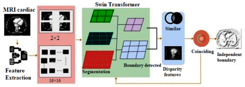
UMSN is a different approach that engages a unique master plan by associating the similar-dimension pixels into segments ranging from 2×2 to 16×16. This segmentation perspective is instrumental in enhancing the accuracy of disease detection. Within this grouped pixel analysis, an indispensable layer is trained using pixels that manifest unanimous feature extraction. This training methodology allows the framework to determine the segment boundaries efficaciously. During the boundary detection procedure, this process organizes the coinciding pixel boundaries with similar features for training the fundamental segment of consecutive boundaries. The UMSN denotes an innovative advancement in cardiac MRI observation for disease detection and diagnosis. By associating the pixels, determining the disparities, and purifying its training process, UMSN contributes importantly to the prior detection of cardiac diseases, which leads to better patient care and results in the realm of smart health. In Figure. 1 the overall process of the proposed network is portrayed.

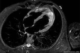
The MRI-Cardiac inputs are taken for further feature extraction operations. From the inputs, the high-quality images contribute precise functionalities that help provide the basement for the subsequent feature extraction operations. Through the proposed advanced image processing operations, the same characteristics and frameworks are extracted for future procedures. These extorted characteristics are necessary for the precise determination of cardiac diseases, which helps detect the diseases in their earlier stages. MRI-Cardiac inputs help in the precise analysis and then the detection of heart-based diseases, producing indispensable insights into the patient’s health. The process of analyzing the MRI-Cardiac inputs for further operation is explained in the upcoming equation:

$\left.\begin{array}{c}\gamma_a=a-2^n \\ \text { if } \frac{2^n}{a} \in N \\ a-2^n \geq 0 \\ \hat{\gamma}=N-\gamma^{n-1} \\ \gamma^{\prime}=\hat{\gamma}+\frac{N}{2}(n * 2) \\ \gamma(N)=\frac{N}{2}\left[\sum_{n=1}\left(\gamma * \frac{n}{2}\right)\right] \\ \gamma_n=\gamma_a+\frac{N}{2}(n * \gamma)\end{array}\right\}$               (1)

where, γ is denoted as the MRI-Cardiac inputs, a is represented as the analysis procedure, and N is represented as the functionalities detected from the inputs. Now the features are extracted from the given MRI-Cardiac inputs. After the determination of the MRI-Cardiac inputs, the feature extraction process is performed which helps in separating and quantifying the distinctive features within the acquired cardiac input images. Features extract the entire information of the input images which includes the textural features. This operation helps in detecting the variations in the structure. In this process, the smoothness, or the tendency of the tissues is derived for further procedures. These characteristics produce valuable insights into the cardiac tissues insane and also help detect the subtle abnormalities that assist the healthcare in diagnosing priory. The process of feature extraction from the detected MRI-Cardiac inputs is explained in the following equation given below:

$\left.\begin{array}{c}\beta=F_a \\ F \in \gamma^{n \times n} \\ a=F^n \beta \\ n \in\{0,1\}^N \\ \hat{\beta}=N \odot \beta \\ \hat{a}=F^n \hat{\beta} \\ \begin{array}{l}=1 \\ =1\end{array}(a)+\gamma\left\|\beta-n \odot\left(F_a\right)^2\right\| \\ a^*=\frac{\gamma_a}{\gamma_\beta} \\ \beta^*=\frac{\gamma_a}{\gamma_{\hat{\beta}}} * \frac{\gamma_{\hat{\beta}}}{\gamma_n} * \frac{\gamma_n}{\gamma_a}\end{array}\right\}$              (2)

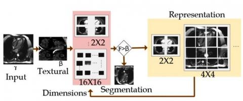
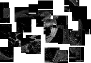
where, $\beta$ is represented as the extraction of the characteristics, and F is denoted as the detected textural features in the acquired inputs. Now the representation of the dimension’s operation is performed. This is the process of denoting the data in both the 2×2 to 16×16 dimensions. This plays an important role in cardiac MRI analysis. This operation engages the structuring of the extracted features and textural information in two distinct dimensions, producing the complete representation of the cardiac data. Therefore, in the 2×2 dimensions, the refined details and localized variations within the acquired input MRI input images are captured. This permits for the more explored assessment of the particular regions of the heart, making it fit for the detection of the irregularities within it. The dimension representation process is illustrated in Figure 2.

The input $\gamma$ is used for extracting $\mathrm{F} \forall \beta$ such that $\mathrm{F} \leq \beta$ condition is to be satisfied. Based on the $\gamma(\mathrm{N})=\frac{\mathrm{N}}{2} \forall \mathrm{n} \in \mathrm{N}$, the $\alpha$ is performed in representing the $\gamma$ at its least and maximum formats. In this representation, the $F$ is validated based on available $\gamma^{\mathrm{n}-1} \forall \mathrm{~N}$ such that $\widehat{\beta}=N \odot \beta$ is the idle condition. Therefore, for the $\mathrm{F} \leq \beta$ satisfying condition, segmentation is pursued (Figure 2). Also, the $16 \times 16$ dimension provides an expanded perspective by integrating the data over larger cardiac image areas. This dimension is important for dehiscing the frameworks and overall cardiac structure and functionalities. By denoting the data in both dimensions, the algorithms assess the comprehensive dataset that associates the refined data with the precision and reliability of cardiac disease detection and diagnosis. This dimension representation improves the utilization of the MRI data in enhancing patient care and its outputs. The process of the dimension representation of the acquired data is explained in the equation below:

$\left.\begin{array}{c}\beta(j)=\left\{\begin{array}{cc}\beta_\gamma(j) & \text { if } j \in N \\ \frac{\beta_\gamma(j)+N_{\widehat{\beta}}(j)}{1+N} & \text { if } j \in N\end{array}\right. \\ F_{\gamma \beta}(a, \beta, \gamma)=F^n+\frac{\gamma}{1+\gamma} F(N \odot \beta) \\ \left\{\begin{array}{c}1 \quad if \, F \notin N \\ \frac{1}{1+\gamma} if \, F \in N \\ \end{array} \right. \\ \frac{\partial F_n}{\partial a_n}=F^n a \gamma \\ F \in N^{n \times n} \\ F \odot N \approx \frac{\gamma}{\beta}\end{array}\right\}$          (3)

where, j represents the dimension representation of the data. Now the SwinTransform process takes place in this MRI analysis procedure. It is used in thwarting the pixel differentiation issued in the MRI cardiac analysis. This process is important in the MRI cardiac analysis particularly designed to address the issues that are related to pixel differentiation. It helps enhance the precision and efficaciousness of disease detection within the cardiac MRI data. In this swim transformer process, the segmentation and boundary detection procedures are performed for further procedures. The SwinTransform process is explained in the equation below:

$\begin{aligned}\left\{F_j^i\right\} & =\operatorname{swirm}\left(I_n\right) \\ n & =1,2,3,4,5 \\ \left\{F_V^i\right\} & =\operatorname{swirm}\left(I_\gamma\right) \\ \gamma & =1,2,3,4,5\end{aligned}$

$\left.\begin{array}{c}I=I_0 * \beta \\ I_1=I_2 * \beta_1 \\ \beta_1=F N \\ a_1=f_1\left(F^N\left(N_1 \odot \beta\right)\right) \\ a_n=f_n\left(F^N\left(N_n \odot \beta_n\right)\right) \\ a_F=a_1+a_n \\ \bar{a}_1=F(N \odot \beta) \\ \bar{a}_n=F_n\left(N_n \odot \beta\right)\end{array}\right\}$            (4)

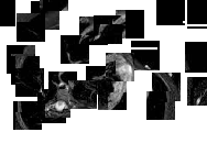
where, I is denoted as the operation of SwinTransform in the further processes. Now the segmentation process is performed in the SwinTransform operation. This algorithm helps in grouping the pixels with similar features into segments, which range from 2×2 to 16×16 in dimensions. By associating similar pixels, the operation reduces the issues and problems based on pixel differentiation. This segmentation process is useful in simplifying the difficult cardiac images, permitting an efficient focused analysis.

$\left.\begin{array}{c}\beta_i=\sum_{n=1}\left(F\left(a_i\right)\right) a_i+a_i \\ \hat{\beta}_i=\sum_{n=1}(F(N-\gamma \odot N-n)) F-N+a_i \\ \beta_i=\sum_{n=1}\left(\gamma N\left(\hat{\beta}_i\right)\right)+\hat{\beta}_i \\ (a, \beta)=1-\frac{2}{N j} \sum_{j=1}^J \frac{\sum_{i=1}^I a_{i j} \beta_{i j}}{\sum_{i=1}^I a_{i j}^2+\sum_{i=1}^I \beta_{i j}^2} \\ \sum_{n=1}(a, \beta)=\frac{1}{I} \sum_{i=1} \sum_{j=1} a_{i j} \log \beta_{i j} \\ (a, \beta)=N(a, \beta)+N_{i j}(a . \beta)\end{array}\right\}$            (5)

$\left.\begin{array}{c}\varepsilon_{i j}=\frac{2 \times|a \cap \beta|}{|a|+|\beta|} \\ \varepsilon_{i j} \leftarrow F_n\left(a_n-1\right) \\ \leftarrow \beta_1 \cdot \gamma_{n-1}+\left(1-\beta_1\right) \\ \gamma_n \leftarrow \gamma_{n-1} \cdot a(\varepsilon+a \beta) \\ \gamma_{i j}=\frac{|a \cap \beta|+i j}{\left|a_{i j}\right|+\left|b_{i j}\right|} \\ \gamma_n=\frac{|a \cup \beta| * i j}{\left|a_{i j}\right|+\left|b_{i j}\right|} \\ F_{i j}=\frac{|a \cap \beta|+i j}{\left|a_{i j}\right|+\left|b_{i j}\right|} \\ F_n=\frac{|a \cup \beta| * i j}{\left|a_{i j}\right|+\left|b_{i j}\right|}\end{array}\right\}$             (6)

These steps assess the meaningful categories to segments based on their distinct features, helping differentiate between the various parts of the heart and surrounding tissues. The segmentation using a SwinTransformer is presented in Figure 3.

1.png

Figure 1. Overall process of the proposed network

2.jpg

Figure 2. Dimension illustration

3.png

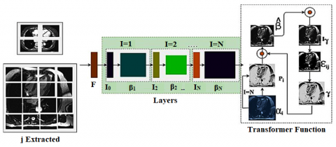
Figure 3. Segmentation process

Algorithm 1 for Segmentation

The extracted j forms the input for the segmentation process in which $\mathrm{I}=1$ to $\mathrm{I}=\mathrm{N}$ layers are split. Based on the split, the segmentation is performed; $\widehat{\beta}$ and $\varepsilon_{\mathrm{ij}}$ validate the transform function for training and validation. Considering the $I_o$ and $\beta_N$ for the j , the layers are trained for the $\left\{\mathrm{F}_{\mathrm{j}}^{\mathrm{i}}\right\}$ until $\mathrm{I}=\mathrm{N}$ is reached. This segmentation varies with $F$ and $j \forall(2 \times 2),(4 \times$ $4), \ldots(16 \times 16)$ instances. The transformer process assimilates $\varepsilon_{i j}$ for $I_\gamma$ and $\widehat{\beta}_i$ provided $\bar{\alpha}_n$ satisfies $F_n\left(N_n \odot \beta\right)$ in identifying a boundary (Figure 3). Segmentation helps in accurately determining the boundaries, structures, and anomalies, easing accurate disease detection and diagnosis. The process of segmentation in the SwinTransform is explained by the following equation given above. The segmentation process is described in Algorithm 1.

Now the boundary detection procedure is performed using the SwinTransform algorithm. The boundary detection operation is established through this technique. After the data is segmented into valuable regions, the technique helps in determining and describing the boundaries that isolate these regions. It does this by assessing the pixel transitions and differences in intensity or the textural features between the adjacent segments. The process of detecting the boundaries is explained in the equation below:

$\left.\begin{array}{c}Z_i=N_i\left(Z_i-1\right)+Z_i-1 \\ Z_i=N_i\left(\left[Z_0, \ldots, Z_{i-1}\right]\right) \\ \gamma=Z^n \\ a=N^\gamma \\ \beta=N^i \\ \text { such that, } \\ Z^n \cdot N^\gamma \cdot N^i \approx 2 \\ Z \geq 1, N \geq 1, N^i \geq 1 \\ Z_{i j}=\frac{|a|+|\beta|}{\left|a \beta_{i j}\right|}\end{array}\right\}$                       (7)

where, Z is denoted as the boundaries detected. By precisely detecting the boundaries, the SwinTransform technique in accurately detecting the structures within the cardiac images, such as the normal functionalities of the heart and its irregularities is analyzed. This information is useful for diagnostic purposes between the cardiac structures which leads to a more understanding of the patients’ cardiac health. Also based on these outcomes, the similar and disparity features are determined for the further necessities.

$\left.\begin{array}{c}V_{i j}=\frac{\sum_{n=1}\left(\frac{-\left\|a_i-a_j\right\|^2}{2 n^2 i}\right)}{\sum_{n \neq v}\left(\frac{-\left\|a_i-a_j\right\|^2}{2 \gamma^2 i}\right)} \\ V_{i j}=\frac{\left(V_{j i}+V_{i j}\right)}{2 n} \\ \gamma_{i j}=\frac{\left(1+\left\|\beta_i-\beta_j\right\|^2\right)^{-1}}{\sum_{n=1}\left(1+\left\|\beta_n-\beta_{i j}\right\|^2\right)^{-1}} \\ Z(Q \| \beta)=\sum_i \sum_j V_{i j} \log \frac{V_{i j}}{\gamma_{i j}}\end{array}\right\}$         (8)

where, V is denoted as the information produced by the SwinTransform procedure. Now similar features are detected from the outcome of the SwinTransform operation. This operation is engaged in determining and classifying the segments or regions that manifest similar characteristics within the cardiac MRI data. Similar features are organized for the analysis of the efficient features from the acquired MRI input images. It enables the technique to determine the consistent frameworks across the different parts of the heart. This feature-dependent approach helps enhance the precision of disease detection and diagnosis, as it permits a better understanding of the regions with shared attributes. The process of detecting the similar features is explained in the equation given below:

$\left.\begin{array}{c}\sigma^n=\frac{1}{V}\left(\sum_{i=1}^V a_i\right) \\ \sigma=\sqrt{\frac{1}{\frac{1}{V} \sum_{i=1}^V\left(a_i-\sigma^n\right)^2}} \\ \sqrt \frac{\sum_{n=1}\left(a_{i j} * \beta_{i j}\right)}{\sum_{n=1}(a+\beta) * \sum_{i=1}\left(\frac{a}{\beta(n)}\right)} \\ \sigma_{i j}\left(\sum_{n=1}(a, \beta)\right)=\frac{1}{2}\left[\sum_{n=1}\left(\frac{1}{V}(a, \beta)\right]\right. \\ \sigma\left(V_{i j}\right)=\frac{1}{2} \sum_{n=1}^n \frac{a_{i j}}{\beta_{i j}(N)}\end{array}\right\}$                    (9)

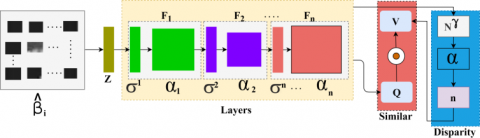
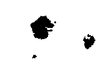
where, $\sigma$ is denoted as the similar features detected from the outcome of the SwinTransform. Now the disparity features are extracted. It involves determining the differences among the detected features and regions [33, 34]. These disparities may manifest as differences in textures or intensities within the segmented and classified data. The boundary detection and the disparity feature classification using the SwinTransformer are illustrated in Figure 4.

4.png

Figure 4. Boundary detection and classification

The SwinTransform model is designed with 1 input and 1 output layers. A N consecutive layer with $I_o$ to $I_N$ and $\beta_1$ to $\beta_N$ with $F$ input is sandwiched between the input and output layers. Based on the validation of $\mathrm{I}=\mathrm{N}, \mathrm{I}$ is incremented by 1 for $I_r$ or $\varepsilon_{i j}$ or $\gamma$ reciprocating to $\left[\alpha_i, P_i \in \hat{\beta}\right]$ differences. Therefore, the initial parameters ($\mathrm{P}_{\mathrm{i}}, \alpha_{\mathrm{i}}$ ) are tuned by I and $\left(\beta_N-\hat{\beta}\right)$ difference until $I=N$ conditiondl. These $N$ layers are dependent on the number of transformer instances required to meet the $\sum j \forall F_n\left(N_n \odot \beta\right)$. The $\widehat{\beta}_i$ inputs are used for the I process in the $\mathrm{F}_{\mathrm{n}}$ and feature classification. The boundary detection process is performed from $F_1$ to $F_n$ layers using $\sigma^n$ and $\alpha_{\mathrm{n}}$ entries matching Z. In this process, the j is required for $\sigma\left(\mathrm{V}_{\mathrm{ij}}\right)$ estimation as in Eq. (9). The normalization using $\frac{\left\|\alpha_{\mathrm{i}}-\alpha_{\mathrm{j}}\right\|}{2 \mathrm{n}^2 \mathrm{i}} \forall \mathrm{i} \in \mathrm{n}$ is used for feature classification acrossN ${ }^\gamma$ for disparity. A similar feature is estimated using $\mathrm{V} \odot \mathrm{Q}$ assessment from $n$ and ($\sigma^{\mathrm{n}}. \alpha_{\mathrm{n}}$) outputs from Z. Therefore, the transformer network requires $F_1$ to $F_n$ for all the possible $\widehat{\beta_1}$ (Figure 4). By separating these disparities, the analysis exhibits the regions that deviate from the criteria. These deviations signify efficient irregularities that need depth evaluation.

$\left.\begin{array}{c}Q=V^Q \times a \\ \gamma=V^\gamma \times a \\ I=V^I \times a \\ \sum_{i j}(Q, \gamma, I)=\left(\frac{Q \times \gamma^T}{\sqrt{d \gamma}}\right) \times Q \\ a^t=V N_1(a) * \beta_1 \\ a^t=V N_2(a) * \beta_2 \\ \beta=a^t \times a \\ Q_{i j}=\left(\frac{\gamma_{i j} * V_{i j}}{(a, \beta)}\right)\end{array}\right\}$                (10)

The disparity features determination operation is explained by the following equation given above. Now the coinciding features are estimated from the feature determination process outputs. This process involves determining the characteristics that coincide with each other across the different regions or segments of the acquired MRI data. These coinciding features represent similar characteristics. The evaluations of the coinciding features are an important strategy for enhancing the precision and reliability of disease detection and diagnosis in the cardiac MRI analysis, as it eases the determination of consistent cardiac features. The process of determining the coinciding features is explained in the upcoming equation:

$\left.\begin{array}{c}a^{t 1}=V N_1\left(a^{V-1}\right)+Q\left(a^{V-1}\right) \\ a^t=V N_2\left(a^{t 1}\right)+Q\left(a^{t 1}\right) \\ a^{t 2}=V N_3\left(a^t\right)+Q\left(a^t\right) \\ V=V N_4\left(a^{t 2}\right)+Q\left(a^{t 2}\right) \\ \frac{a^V}{a^{i j}}=\frac{2| | a \cap \beta \|}{||a||+\|\beta\|} \\ =\frac{2 \gamma}{2 \gamma+F V+F N}\end{array}\right\}$             (11)

$\left.\begin{array}{c}\varphi_i=a_i \times Q^{\varphi} \\ V_i=a_i \times Q^V \\ F_i=a_i \times Q^F \\ \beta_Q=\beta_V \\ a_{i j}=\sum_{n=1}\left(\frac{Q_{i j}^1}{\sqrt{V_n}}\right) \\ =\frac{\sum_{n=1}\left(\frac{a_{i j}^1}{\sqrt{V_n}}\right)}{\sum_{j=1}\left(\frac{a_{i j}^1}{\sqrt{V_n}}\right)} \\ a_{i j}^1=Q_i \times V^T\end{array}\right\}$              (12)

where, Q is denoted as the disparities in the features, $\varphi$ is denoted as the coinciding features. Now the training is provided based on the coinciding features of the SwinTransform procedures. During this operation, the algorithm technique understands the determined coinciding features that denote consistent patterns within the detected MRI data. These features help as important training, enabling the process to efficacious understanding and to categorize similar patterns in MRI scan outputs. By training on coinciding features, the SwinTransform operations become more adept at determining and interpreting irregular conditions, improving accuracy and diagnostic capabilities. The process of providing the training the SwinTransform is explained in the following equation:

$\left.\begin{array}{c}A V_i=\int_0^1 V_i\left(Q_i\right) d Q_i \\ I o V=\frac{a \cap \beta}{a \cup \beta} \\ V_{a \beta}=\frac{\sum_{n=1} A V_i}{n} \\ \epsilon_{i j}=\frac{1}{T} \\ A V_{i j}=\int_0^1 \frac{V_i}{\gamma_i}\left(Q_i\right) * \int_0^1 Q_{i j} \\ V(Q * N)=\frac{a \cap \beta}{a \cup \beta} * N\left(\frac{\gamma \cup \beta}{\gamma \cap \beta}\right)\end{array}\right\}$            (13)

where, ϵ is denoted as the training provided based on the determined coinciding features. Now the independent boundary is determined based on the prior process outputs. Independent boundaries exhibit unique characteristics or differences, distinct from the coinciding features [35]. This identification helps the technique to determine the boundaries that represent the particular cardiac structures, enhancing the precision of the analysis. The process of extracting the independent boundary as per the previous process is explained by the following equation given below:

$\left.\begin{array}{c}\mu_0=\left[F_1+V_1, F_2+V_2+\cdots+F_n+V_n\right] \\ Q_i \leftarrow \beta_{i-1}, V_i \leftarrow \beta_{i-1}, F_i \leftarrow \gamma_{1+1} \\ V_i=\frac{\left(Q_i-V_i\right)}{\sqrt{N / N_T}} \cdot V_i \\ \beta_i=\operatorname{VN}\left[\left(\beta_i^*\right)+\left(\beta_{i j}^*\right)\right] \\ \text { where } i=1, \ldots, N \\ \beta_n=\frac{\left(Q_n-V_n\right)}{\sqrt{V / V_T}} \cdot V_n \\ \beta_{i j}=\left(\frac{Q_{i j} \cdot V_{i j}}{\sqrt{V / V_{i j}}}\right)\end{array}\right\}$             (14)

where, μ is represented as the independent boundary detected from the analysis process. The overall algorithm of the feature classification is presented as Algorithm 2.

Algorithm 2 for Feature Classification

This process helps in precise analysis of the MRI-Cardiac inputs. It also helps in mitigating the issues in the MRI-cardiac analysis. The SwinTransform helps in accurate segmentation and boundary detection operations. From that, the similar and disparity features are estimated to provide the training for it. The independent boundaries are detected which is free from flaws post the training production process.

Apart from the experimental analysis discussed above, this section presents the accuracy, precision, false rate, classification, and differentiation error as a comparative study. The number of segments (1 to 11) and features (1 to 14) are varied for verifying the proposed network process across each improvement. For this comparative study, the allied methods considered are FCDNet [28], MMNet [21], and TAUNet [22]. The methods are discussed in the related works session.

The accuracy is enhanced in this method with the help of the SwinTransform method. The association of the SwinTransform method importantly improves the accuracy of the cardiac MRI analysis. This process estimates the several difficult issues that often lead to more reliable and precise results. SwinTransform pixel association and segmentation methods streamline the analysis, mitigating the risk of pixel differentiation issues. Classifying the pixels into valuable segments, permits for a more focused evaluation of the cardiac data, mitigating the irrelevant information. The SwinTransform helps determine the similar features and disparities within the acquired MRI data. It also secures the subtle frameworks and dissimilarities mitigation which help in enhancing the accuracy of the procedure. This accuracy is necessary for prior disease detection, where the small difference is indicative of the cardiac conditions. The estimation of the coinciding features and then the training on them enhances the understanding of the method, enabling it to determine consistent cardiac patterns (Figure 5).

5a.png

5b.png

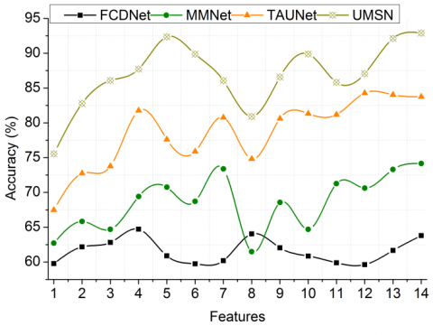
Figure 5. Accuracy analysis

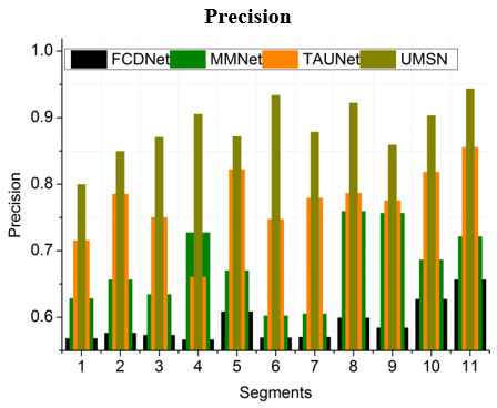
The precision is high in this process with the appropriate segmentation and boundary detection operation. Precision in cardiac MRI analysis is huge, as it directly affects the precision of disease detection and diagnosis. The SwinTransform algorithm pixel segmentation ensures that the cardiac images are separated into valuable segments, mitigating the irrelevant information. This accurate segmentation allows for the main analysis, improving the accuracy of the detection and characterizing the particular regions within the heart. The feature detection precision is also enhanced during this operation which excels in detecting and extracting the characteristics with high precision. It also detects the subtle differences in textures and its intensities. The method's ability to detect the independent boundaries with accuracy is important. It secures the cardiac structures and depth irregularities are precisely defined, mitigating the risk of oversight in this MRI analysis. This operation significantly enhances the precision in identifying and classifying cardiac conditions (Figure 6).

6a.png

6b.png

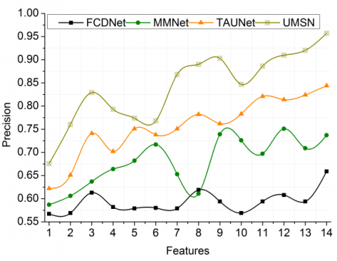
Figure 6. Precision analysis

7a.png

7b.png

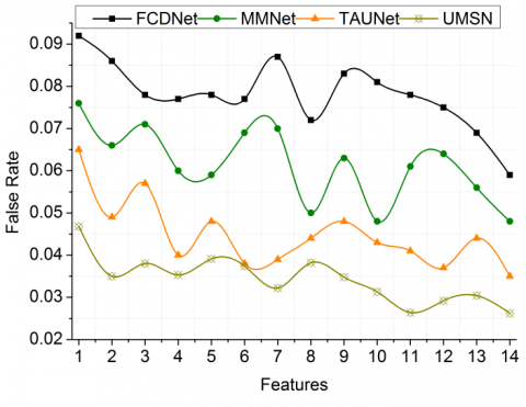
Figure 7. False rate analysis

The false rate is lesser in this process after detecting the similar and disparity features from the output of the SwinTransform operation. Exhibiting a lower false rate results in a substantial improvement in accuracy and reliability. By determining and classifying similar features within the cardiac MRI data, the system becomes perfect at determining consistent patterns. This mitigates the irregularities, which results in a significant reduction in the false positive rates. The extraction of the disparity feature is also helpful in enhancing the reduction of the inconsistencies and variations within the data, permitting the system to showcase the areas that are deviating from the measures. This results in less production of the false negatives with the enhanced MRI analysis. Training the approach on coinciding and disparity features further improves its capacity to differentiate between normal and abnormal cardiac conditions. This clarified understanding importantly mitigates the false rates where the process becomes more discerning in its assessments (Figure 7).

8a.png

8b.png

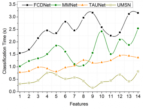
Figure 8. Classification time analysis

The time taken for the classification is less in this method using the SwinTransform algorithm. The integration of the SwinTransform in this method importantly mitigates the time needed for the classification tasks. This approach to pixel grouping and feature extraction streamlines the data analysis operation, making it more efficacious and quicker. Classifying the pixels into valuable segments and aiming at pertinent characteristics, mitigates the need for extensive resources and time-consuming manual interventions. Furthermore, the SwinTransform method’s capability to determine the similarities and disparities within the data improves the categorization operation by establishing a more clarified dataset for the analysis. This efficiency permits the healthcare to obtain timely results according to the presentation of the MRI state. It helps in disease diagnosis and treatment planning for better results within a short time. The reduced classification time helps in the establishment of quicker assessments, providing improved healthcare outcomes (Figure 8).

9a.png

9b.png

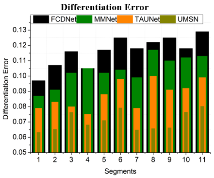
Figure 9. Differentiation error analysis

The differentiation error is lesser in this process after the precise determination of the features from the SwinTransform operation. The pixel grouping, segmentation, and feature extraction procedures enhance the overall accuracy of the cardiac MRI analysis. Classifying the pixels into meaningful segments and boundaries reduces the risk of errors arising from pixel differentiation issues. It also ensures that the data is interpreted with precision. The system’s capability to determine and utilize the same and disparity features further refines its assessment of the data, mitigating the similarities misinterpretation. This process involves determining the characteristics that coincide with each other across the different regions or segments of the acquired MRI data. These coinciding features represent similar characteristics. During this operation, the algorithm technique understands the determined coinciding features that denote consistent patterns within the detected MRI data and thus it mitigates the differentiation errors in the operation (Figure 9). Table 8 and Table 9 presents the comparative analysis results with their discussion.

The proposed UMSN improves accuracy and precision by 9.123% and 9.96% respectively. This method reduces false rate, classification time, and differentiation error by 9.97%, 11.29%, and 10.04% respectively.

The proposed UMSN improves accuracy and precision by 9.5% and 10.53% respectively. This method reduces false rate, classification time, and differentiation error by 10.57%, 10.87%, and 10.86%, respectively.

Table 8. Comparative analysis results for segments

Table 9. Comparative analysis results for features