Zhaoyang Song | Wei Wu* | Hao Wu | Yongshuai Guo | Chao Man
© 2025 The authors. This article is published by IIETA and is licensed under the CC BY 4.0 license (http://creativecommons.org/licenses/by/4.0/).
OPEN ACCESS
As a common algorithm in the field of image denoising, convolutional sparse self-coding has the defect of weak adaptability to images with different noise levels. Aiming at the difference of image noise le vel and the existing noise level estimation algorithms, an image denoising algorithm is proposed, which combines noise estimation and convolution sparse self-coding. This algorithm first estimates the noise level of the noise image, and then designs a prior estimation subnet for the noise level. In the subnet, a set of weights are obtained by nonlinear transformation of the noise level using a fully connected neural network, and the noise prior feature map is obtained by multiplying the weights by the components of image wavelet transform. Finally, the noise picture and the noise prior feature map are fused by channels, and then the sparse convolutional self-coding network is used for noise reduction, so as to effectively improve the noise reduction effect of the convolutional sparse self-coding noise reduction network.
image denoising, convolutional neural network, sparse self-coding, noise level, wavelet transform, noise prior
Image denoising means a series of conversion operations on the noisy image, and the details of the image are restored as much as possible on the basis of removing the image noise. Image denoising is a basic task of computer vision, which can be effectively used in high-order tasks such as image segmentation, target detection and tracking in computer vision. In the process of noise reduction, two operations need to be completed, that is, removing noise and restoring details. However, these two operations are opposite to each other to some extent, that is, excessive noise removal tends to make the image too smooth and lose detail information, and retaining details mainly often leaves a lot of noise. Therefore, image denoising has received extensive attention from the industry because of its complexity.
The design of image denoising algorithm has mainly gone through three stages [1], namely, filter-based denoising algorithm, model-based generative denoising algorithm and discriminant denoising algorithm based on deep learning. Early image denoising mainly used filter-based denoising algorithm, that is, using a global filter to convolution the image and filtering the noise by weighting. Common filters include median filter [2], Gaussian filter [3] and bilateral filter [4]. The noise reduction algorithm based on filter is simple in design and fast in noise reduction, but the noise reduction effect is relatively poor. Model-based denoising algorithms are generally modeled according to some prior characteristics of images. Typical model-based denoising algorithms include BM3D algorithm [5] and WNNM algorithm [6]. Among them, BM3D algorithm takes the spatial similarity of images as a priori and uses block verification to model; WNNM algorithm takes the low rank of the image as a prior, maps the image to a low rank subspace by using dictionary modeling, and then experiments the image denoising. The model-based denoising algorithm is generally stronger than the filter-based denoising algorithm, and has strong robustness, but it takes a long time to denoise. The image denoising algorithm based on deep learning generally adopts discriminant modeling, that is, a large number of noise and real pictures are trained by neural network, and the parameters are updated by error back propagation, and then the corresponding denoising model is obtained. With the deepening of the research on deep learning algorithms, some research results in the field of deep learning have been applied to the task of image denoising. IRCNN [7] combines stacked convolution layers and introduces adaptive mechanism to deal with image restoration with diverse scales and complexity. The model dynamically adjusts the weight according to the pixel context, which improves the flexibility and accuracy of processing. Ducknn [8] mainly adopts the methods of residual learning [9] and batch normalization to improve the denoising ability and training speed of the model. FFDNet [10] adopts U-Net architecture with adaptive weight module, and combines nonparametric mean variance estimation to accurately predict pixel-level noise. Through batch normalization and batch training, FFDNet realizes real-time performance of single GPU. CBDNet [11] adopts real noise model, which integrates Poisson-Gaussian distribution, signal-dependent noise and ISP influence. Asymmetric loss function is used to improve the generalization ability of the network, and synthesis and real noise image training are combined to adapt to the real scene. RIDNet [12] introduces residual learning on the basis of residual network structure, and uses two residual connection methods, local connection (LC) and long skip connection (LSC), to dynamically adjust the weight of feature map. The core innovation of NBNet [13] is to propose a noise-based learning method, and skillfully use subspace projection technology and self-attention mechanism [14] to separate and remove image noise. Unlike traditional denoising methods that rely on complex network structures, NBNet focuses on deeply understanding and utilizing the inherent characteristics of noise. DeamNet [15] introduces nonlinear filter operator, reliability matrix, sparse self-coding [16] and high-dimensional feature transformation function to construct adaptive consistency prior. This prior is good at dealing with complex noise patterns, dynamically adjusting the filter strength, and mining more useful information from multiple scales and angles, effectively preserving the image structure and accurately removing noise. FADNet [17] is based on the improvement of two-dimensional convolution of encoder-decoder architecture, which integrates residual structure and point-by-point correlation convolution to enhance the ability of feature extraction and expression. Multi-scale residual learning strategy and weighted loss method are adopted to realize model training from coarse to fine. The above-mentioned image denoising algorithm based on deep learning has made some achievements in image denoising, but there are still some aspects that can be improved. First of all, the current mainstream noise reduction algorithms generally use sparse convolutional self-coding network as the main framework of noise reduction network, which can conveniently realize the end-to-end mapping of image noise reduction, but the use of noise information is relatively limited. Secondly, the image noise level can clearly reflect the degree of image damage, and help the noise reduction network to use parameters reasonably to preserve the image details as much as possible, thus effectively improving and reducing the over-fitting degree of the noise reduction network. Although some of these algorithms try to use noise subnet to estimate the noise subgraph of the image, they do not effectively use the key index of image noise level. In order to solve the problem of using noise information by sparse self-coding as the mainstream framework of image denoising, noise level can be actively integrated into sparse self-coding network as noise prior information to improve network performance. For the estimation of image noise level, Chen et al. [18] proposed a nonparametric noise level estimation algorithm based on principal component analysis, and achieved accurate prediction results in Gaussian additive noise images. However, how to effectively convert the noise level of a single numerical value into the prior information of image noise and how to effectively integrate the prior information with the noise reduction network has become a research difficulty. In order to solve the problem of effective integration of noise level and noise reduction network, this paper proposes a noise prior extraction network for noise level, and integrates noise prior information into noise reduction network to make full use of noise level information. The main contributions include the following points:
1) A fully connected network is used to map the estimated noise level into four noise weights, and at the same time, the image is decomposed into four components by HAAR wavelet transform. After multiplying the weights, the noise prior feature map of the image related to its own noise level is obtained by inverse transformation.
2) The image information and the noise prior feature map are effectively fused by the way of channel cascade, and a sparse convolutional encoder is designed to train the fused result for noise reduction, so as to obtain a noise reduction model.
3) The effectiveness of the test algorithm is verified on Gaussian additive data set and real noise data set respectively. The experimental results show that compared with the original image input, the input fused with prior features can effectively improve the noise reduction effect, and the best results can be obtained in comparison with the noise reduction effect of the current mainstream noise reduction algorithms.
2.1 Noise level estimation algorithm
Gaussian noise estimation algorithm based on principal component analysis uses the low rank characteristics of noise-free blocks to model. For a picture x∈RC×H×W, where C represents the number of channels of the picture, H represents the width of the picture, and W represents the height of the picture. In this algorithm, the picture is divided into 8×8 sizes and then spliced into a picture block matrix y∈RM×N, where M=C×8×8. The picture blocks are converted into a one-dimensional vector, and N=(H-8+1)(W-8+1) represents the number of cut picture blocks. Then the covariance matrix of the picture block is decomposed into eigenvalues to obtain an eigenvalue vector, and the calculation method is shown in Eq. (1):
e=γ(Φ(y−u)(y−u)T) (1)
where, u=1n∑Ni=1yi is the mean vector of y. Φ represents the eigenvalue decomposition function, which returns the eigenvalue of a square matrix. γ represents a sorting function, that is, sorting the eigenvalues in order from largest to smallest. Noise estimation is to find a suitable value from e. Two lemmas are given for this algorithm. First, for a group of random variables {nt[i]st=1}, if each element follow standard normal distribution independently and identically, the estimated noise level ˜σ2=1s∑St=1nt[i]2 converges to N(σ2,2σ4s) when s is large. Secondly, for a vector xt∈Xs in M-dimensional space, suppose that M satisfies the following conditions:
m<r−(1−2α)δ(β)+α1−δ(β) (2)
δ(β)=Φ((1+1β)Φ−1(0.5+β2)) (3)
where, β=mr, the mean value of the set is approximately equal to the median value when m is 0 or there is no large outlier in the set. Finally, the algorithm calculates the eigenvalue vector, and continuously removes large eigenvalues from the eigenvalue vector until the average value of the eigenvalue vector is equal to the median position. The square root of the median in this set is the noise level of the picture.
2.2 Convolutional sparse self-coding
Convolutional sparse self-coding is often used in image reconstruction tasks, such as image denoising, image defogging and super-resolution tasks. Convolution sparse self-coding is to replace the fully connected layer of the original sparse self-coding with 2D convolution layer on the basis of sparse self-coding. The general structure of convolutional sparse self-coding for image denoising is shown in Figure 1.
Figure 1. Image denoising convolution sparse self-coding general network structure
According to Figure 1, convolutional sparse self-coding generally consists of an encoder and a corresponding decoder. Image data is encoded by a group of coding layers consisting of a convolutional layer and an activation layer, and each coding layer is compressed by spatial pooling of the picture. Common pooling methods include maximum pooling, average pooling and using a convolutional layer with a step size greater than 1. This compression method is similar to reducing the number of hidden layers in sparse self-coding to obtain bottleneck features. The feature map after multiple encoding layers will be decoded through a series of decoding layers. The decoding layer is the reverse operation of the corresponding coding layer, and its network structure is similar to that of the coding layer. The difference is that compared with the coding layer's scaling of the spatial level of the feature map, the decoding layer needs to restore the spatial level of the feature map, and generally uses bilinear interpolation or deconvolution layer with a step size greater than 1 to operate. Each coding layer and the corresponding decoding layer are generally connected by residual method to ensure the effective transmission of feature map information and prevent the gradient from disappearing during network training.
3.1 Main structure of self-coding network integrating noise prior and convolution sparse
After the prior information of noise is extracted, it will be further integrated into the information of the noise picture itself, and then the sparse convolutional self-coding network is used to reduce noise. The main structure of the noise reduction network is shown in Figure 2. The network mainly consists of two parts: the noise prior estimation subnet and the noise reduction network. The input noise picture first passes through the noise prior subnet to obtain the noise prior feature map, and then it will be further fused with the noise image. Because the prior feature map does not fuse the images of each channel in the extraction process, the fusion between the prior feature map and the noise image still uses the fusion method for each channel. The fusion mode is that the prior feature image and the noise image are respectively spliced according to each channel and then spliced at the same place, and then the depth-separable convolution layer [19] is used for fusion, and the fusion among channels is realized by setting the number of convolution groups equal to the number of channels.
Figure 2. Main structure of noise reduction network
The noise reduction network is based on convolutional sparse self-coding, and the algorithm in this paper uses four coding layers and four decoding layers. Residual connection is used between each coding layer and the corresponding decoding layer to prevent gradient disappearance during training. The encoder includes a series of 3×3 convolution layers and Relu layers for feature extraction, and a 1×1 convolution layer is connected with the residual to scale the features. The pooling layer uses a convolution layer with a step size of 2. The decoder first uses a deconvolution layer [20] with a step size of 2 to expand the image, and then uses a series of 1×1 convolution layers and Relu layers to extract features and connect a 1×1 convolution layer to output. In the network training process, the mean square error is used as the loss function of the noise reduction network, and the calculation method of the mean square error is shown in Eq. (4).
L(θ)=1H×W×C∑Hi=1∑Wj=1∑Ck=1[Θ(x)ijk−yijk] (4)
where, x∈RC×H×W represents the noise image, y∈ RC×H×W represents the real image and Θ(x) represents the output of the noise reduction network.
3.2 Noise prior estimation subnet
In order to effectively fuse the noise level and noise image information, this paper proposes a noise prior estimation sub-network, which is the Prior Subnet module in Figure 2. The network structure is shown in Figure 3.
Figure 3. Subnet structure of noise prior estimation
The noise prior estimation subnet first calculates the noise variance of the noise image using the noise level estimation algorithm [18] to obtain the noise level represented by a single floating point number. Then the noise level is nonlinear transformed by a series of fully connected layers and Relu activation layers, and then output by Sigmoid function, which is mapped into four weight values. At the same time, the noise image is transformed by Haar wavelet to obtain four components of the image, and the weight values obtained by noise level are multiplied by these four components respectively, so as to realize the fusion of noise level and image. Finally, the fused image is transformed by Haar wavelet to obtain the noise prior feature map. The noise prior used in this paper is the noise level, and the noise level has been mapped by the fully connected network and changed into a prior weight. The product of this weight and wavelet components means that the prior information is integrated into wavelet components, and the inverse wavelet transform means that these wavelet components integrated with the prior information are converted into a prior feature map consistent with the size of the input image.
For noisy pictures x∈RC×H×W, where c is the number of image channels, and h and w are the height and width of the image respectively, the calculation method of noise prior feature map is shown in Eq. (5).
y=ω−1(ψ(σ)⊙ω(x)) (5)
where, ω(x)∈R4×C×H2×W2 is the result of wavelet transformation of noise map, ω−1 represents the inverse wavelet transformation, and ψ(σ)∈R4×1×1×1 is the result of nonlinear transformation of noise level σ, ⊙ represents the product of matrix element by element. Finally, the size of the noise prior feature map y∈RC×H×W is consistent with the noise picture x. Haar wavelet transform can decompose the picture signal into sub-signals with different frequencies, and the sub-signals between different noisy pictures have certain differences. Aiming at the differences between sub-signals and noise levels, the goal of noise prior estimation network is to balance these differences by using weights. By performing a series of linear transformations on the noise level and mapping it into four different weights, the representation of different components of wavelet transform under different noise levels is controlled to balance. Because Haar wavelet transform itself is reversible, using inverse transform after weighting will get a feature map with the same size of the original picture, which can fuse the picture information and noise level information.
4.1 Experimental data set and evaluation index
4.1.1 Experimental data set
The experiment mainly includes two parts: training and testing of image denoising network. The training part includes waterloo exploration database [21] and SIDD-medium [22] data sets. The Waterloo Exploration Database data set contains 4744 real pictures. In order to unify the training size, these 4744 pictures are randomly cropped, that is, the fixed-size picture blocks are cut from any position in the original picture, the cropping size is set to 128×128, and the cropping number is 80000. Then Gaussian noise with noise level evenly distributed in [5,75] is added to these picture blocks to form a true and noisy picture pair. For the original picture x∈R3×H×W, where h and w are the height and width of the image. The noise picture synthesis mode can be expressed by Eq. (6).
y=x+n (6)
where, y∈R3×H×W is the image after adding noise, n∈R3×H×W is Gaussian white noise, and its standard deviation is noise level. SIDD-medium data set contains 320 real noise and corresponding original picture pairs, from which 300 pictures will be randomly cropped to get 20,000 128×128 picture patchs. Gaussian noise image pairs and real noise image pairs are fused to obtain a training set, which contains 100,000 image pairs in total. On the basis of Gaussian noise, real noise is further integrated for training to improve the robustness of the model to different types of noise. The data sets used in the test set of the experiment mainly include BSDS200 [23], Manga109 [24] and T91 [25]. Among them, BSD200 contains 200 pictures in JPG format, Manga109 contains 109 comic cover pictures in PNG format, and T91 contains 91 pictures in PNG format. The pictures in the above three data sets are all original real pictures. The test set data adds a certain level of Gaussian noise to these data sets. Experiments will verify the noise reduction effect of the algorithm when the noise level is 25 and 50 respectively. In order to further verify the denoising effect of the algorithm proposed in this paper on real noise pictures, the remaining 20 real noise pictures in the SIDD-medium data set and RNI15 data set [26] were selected as the data sets for testing real noise. Among them, RNI15 contains 15 pictures with real noise. Because there is no corresponding original real picture, the experimental results will be presented with visual noise reduction effect.
4.1.2 Implementation scheme
The number of dense layer nodes from front to back in the noise prior feature extraction network is set to 10, 10 and 4 respectively. The number of channels output by the four coding layers of the noise reduction network is set to 64, 128, 256 and 512 respectively, in which the scaling ratio of the pooling layer is 1/2, and the number of channels output by the four decoding layers is set to 256, 128, 64 and 32 respectively, and the expansion ratio of the deconvolution layer is 2. The batch size of network training is set to 16, the number of iterations is set to 80000, and the initial learning rate is set to 0.001. During the training process, the learning rate is updated to 0.0001 when the loss does not decrease any more, and ADAM algorithm [27] is used for optimization.
4.1.3 Evaluation indicators
In this paper, Peak Signal-to-Noise Ratio (PSNR) and Structural similarity (SSIM) are used as evaluation indexes of network noise reduction effect, and the calculation method of PSNR is shown in Eq. (7).
PSNR=10log10(MAX2yMSE) (7)
where, MAX2y represents the square of the maximum pixel value of the real image y, and MSE is the mean square error, and the calculation method is shown in Eq. (8).
SSIM(x,y)=(2uxuy+c1)(2σxy+c2)(u2x+u2y+c1)(σ2x+σ2y+c2) (8)
where, ux and uy respectively represent the mean value of the sum of the compared images x and y,σx and σy represent the variances of x and y respectively, and σxy represents the covariance between them.
4.2 Analysis of experimental results
4.2.1 Comparison of noise reduction effects of gaussian additive noise
The PSNR and SSIM values of noise reduction effects of BSDS200, Manga109 and T91 are shown in Table 1, where σ represents noise level, Params represent the number of network parameters in millions, and Infer Time represents the inference time of the network for a single picture with a size 320×320. Ours indicates that according to Table 1, CBM3D algorithm, as a model-based noise reduction algorithm, has a weak overall noise reduction effect. The other algorithms are the current mainstream noise reduction algorithms based on deep learning, and the overall noise reduction effect is relatively good. Among them, the algorithm proposed in this paper has achieved the best results in PSNR and SSIM indexes compared with many mainstream algorithms. The parameters of IRCNN, DnCNN, FFDNet and RIDNet are relatively few and the noise reduction takes relatively short time. DeamNet involves several sparse self-encoder iterations, while NBNet involves a large number of projection modules, with a relatively large number of parameters and a relatively long time-consuming noise reduction. FADNet, CBDNet and the algorithm proposed in this paper have relatively moderate parameters, and the noise reduction takes relatively short time. The noise reduction time of this algorithm is about 0.96s, in which the noise estimation time is about 0.71s and the network reasoning time is about 0.25s.
Table 1. Noise reduction effects of various algorithms on BSDS200, Manga109 and T91 data sets
|
Method |
\boldsymbol{\sigma=25} |
\boldsymbol{\sigma}=\mathbf{5 0} |
Net Params (M) |
Time Cost (s) |
||||
|
BSD200 |
Manga109 |
T91 |
BSD200 |
Manga109 |
T91 |
|||
|
PSNR/SSIM |
PSNR/SSIM |
PSNR/SSIM |
PSNR/SSIM |
PSNR/SSIM |
PSNR/SSIM |
|||
|
CBM3D [5] |
30.83/0.875 |
30.96/0.876 |
29.88/0.852 |
27.53/0.775 |
27.63/0.775 |
26.58/0.741 |
- |
4.17 |
|
IRCNN [7] |
31.70/0.880 |
31.89/0.883 |
30.81/0.857 |
27.78/0.782 |
27.89/0.786 |
27.08/0.752 |
0.45 |
0.96 |
|
DnCNN [8] |
31.77/0.885 |
31.88/0.885 |
30.91/0.869 |
27.78/0.782 |
27.96/0.783 |
27.05/0.756 |
0.56 |
0.75 |
|
FFDNet [10] |
31.85/0.881 |
31.96/0.882 |
31.03/0.865 |
27.85/0.785 |
28.12/0.785 |
27.17/0.768 |
0.48 |
0.89 |
|
CBDNet [11] |
32.12/0.883 |
32.12/0.887 |
31.27/0.885 |
28.12/0.798 |
28.28/0.797 |
27.32/0.771 |
4.34 |
1.13 |
|
RIDNet [12] |
32.18/0.885 |
32.45/0.901 |
31.33/0.892 |
28.18/0.795 |
28.33/0.795 |
27.98/0.805 |
1.49 |
0.95 |
|
DeamNet [15] |
32.35/0.887 |
32.63/0.902 |
31.65/0.905 |
28.28/0.807 |
28.39/0.810 |
28.27/0.810 |
11.12 |
1.85 |
|
NBNet [13] |
32.43/0.892 |
32.54/0.901 |
31.62/0.902 |
28.28/0.812 |
28.38/0.808 |
28.24/0.805 |
13.3 |
1.75 |
|
FADNet [17] |
32.44/0.895 |
32.62/0.908 |
31.67/0.910 |
28.30/0.811 |
28.39/0.808 |
28.31/0.811 |
2.59 |
0.73 |
|
Ours |
32.51/0.901 |
32.71/0.917 |
31.70/0.912 |
28.33/0.815 |
28.43/0.812 |
28.35/0.828 |
6.87 |
0.96 |
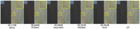
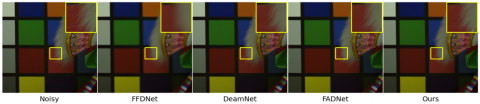
Figure 4 shows the visual effect of current mainstream denoising algorithms on image denoising in BSDS200, Manga109 and T91 data sets. Where Noisy stands for noise picture, and the noise levels is 25 and 50, respectively. GT stands for the original real picture. Ours represents the algorithm proposed in this paper. The values above all kinds of algorithms are PSNR values of noise and noise-reduced pictures and real pictures.
According to Figure 4, there is obvious distortion in the noise reduction image of FFNDNet algorithm, and the effect of preserving the details of the image is slightly weak. The other algorithms can effectively remove noise while preserving the details of the picture. Compared with other algorithms, the algorithm proposed in this paper can better preserve the details of pictures. For example, in the comparison of Figure 4(a), the algorithm proposed in this paper can better reflect the details of insect leg joints, and the PSNR values obtained by this algorithm are the highest. Because the training set used by the algorithm proposed in this paper takes the pictures in Waterloo Exploration Database and SIDD-medium data set as training labels, and Gaussian noise is added as input, the algorithm can achieve good results in noise reduction of additive Gaussian noise, and can also adapt to the noise reduction of real noise. However, for other noises, such as underwater channel multiplicative noise, salt and pepper noise and other noises which are quite different from Gaussian noise, the algorithm proposed in this paper may have certain limitations. Therefore, we will consider designing a noise reduction algorithm that can adapt to various types of noise in the future. It can effectively identify and achieve better noise reduction effect for different types of noise.
(a)
(b)
(c)
Figure 4. Visualization effect of mainstream denoising algorithm on image denoising in BSDS200, Manga109 and T91 data sets; (a) BSDS200 data set; (b) Manga109 data set; (c) T91 data set
4.2.2 Comparison of noise reduction effects of real noise
In the experiment, 20 pairs of real noise and original image were reserved for the SIDD-medium data set to verify the denoising effect of real noise. The PSNR and SSIM values of noise reduction effects of various mainstream algorithms on this test set are shown in Table 2. According to Table 2, compared with various mainstream algorithms, the algorithm proposed in this paper has achieved the best results for PSNR and SSIM in the comparison of real noise data sets. Compared with the suboptimal FADNet algorithm, the algorithm proposed in this paper has improved PSNR and SSIM by 0.03dB and 0.005 respectively.
Table 2. Noise reduction effects of various mainstream algorithms in SIDD data sets
|
Method |
CBM3D [5] |
IRCNN [7] |
DnCNN [8] |
FFDNet [10] |
CBDNet [11] |
RIDNet [12] |
DeamNet |
NBNet [15] |
FADNet [17] |
Ours |
|
PSNR |
31.65 |
38.58 |
38.56 |
38.61 |
38.78 |
38.71 |
39.85 |
39.82 |
39.96 |
39.99 |
|
SSIM |
0.875 |
0.902 |
0.901 |
0.902 |
0.905 |
0.905 |
0.912 |
0.908 |
0.915 |
0.920 |
The visual comparison of noise reduction between SSID and RNI15 data sets is shown in Figure 5. According to Figure 5(a), all kinds of algorithms can obviously improve the PSNR value in the aspect of noise reduction effect. Among them, the noise reduction result of FFDNet is too smooth and the noise reduction effect is relatively weak. Other algorithms can suppress noise on the basis of preserving the details of the picture, and the PSNR of this algorithm is relatively high. The noise reduction effects of various mainstream algorithms in RNI15 real noise data set are shown in Figure 5(b). RNI15 data set only has noise images, so it only gives a visual comparison of noise reduction. Among them, the noise reduction effect of FFDNet algorithm is slightly weak, and the other algorithms can restore the details of the picture well, among which the algorithm in this paper has the most delicate effect on the details of the feathers in the picture.
(a)
(b)
Figure 5. Noise reduction effect of real noise data sets of various mainstream algorithms; (a) SSID data set; (b) RNI15 data set
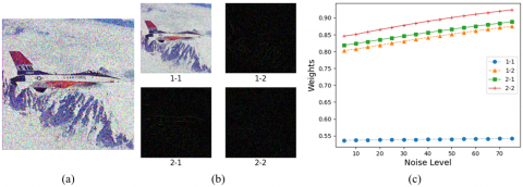
Figure 6. Haar wavelet transform results and weights of feature maps of each component of wavelet transform; (a) the original drawing; (b) wavelet transform feature map; (c) the weight of each feature map
4.3 Ablation analysis
Figure 6 shows the results of Haar wavelet transform and the Weights of the image prior extraction network to the feature maps of each component of Haar wavelet transform under various Noise Levels, where the noise level in Figure 6(c) represents the noise level between 5 and 75, and the weights represent the corresponding weights. According to Figure 6(c), the weights of each feature map of Haar wavelet transform are different to some extent. For component 1-1, which contains a lot of original image information, the weight value is relatively low and stable under different noise levels. For other components 1-2, 2-1 and 2-2 containing a lot of noise information, the weight value is relatively high and has an obvious growth trend with the increase of noise level. This shows that the noise prior estimation network proposed in this paper can properly distinguish noise information from real image information, and is sensitive to different noise levels.
In order to further verify the influence of image noise prior on noise reduction effect, the experiment will compare the noise reduction effect of only using convolutional sparse self-coding network (BaseLine) and noise reduction algorithm (Baseline_Pro) with noise prior, and the PSNR and SSIM values of Gaussian additive noise with noise levels of 25 and 50 for BSDS200, Manga109 and T91 and SIDD real noise after noise reduction are shown in Table 3.
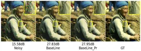
According to Table 3, for Gaussian noise reduction, the noise reduction algorithm with noise prior can effectively improve the noise reduction effect on the basis of convolutional sparse self-coding, which shows that the feature map extracted by the noise prior network proposed in this paper can effectively fuse noise pictures and contribute to the improvement of noise reduction effect. At the same time, for real noise reduction, compared with convolutional sparse self-coding noise reduction network, noise prior can also effectively improve the noise reduction effect. The visual results of noise reduction effects of BaseLine and BaseLine_Pr are shown in Figure 7. According to the PSNR value in Figure 7, the noise reduction effect can be effectively improved after incorporating the prior characteristics of noise.
Table 3. Noise reduction effects of Baseline and Baseline_Pr on BSDS200, Manga109, T91 and SIDD
|
Method |
\boldsymbol{\sigma=25} |
\boldsymbol{\sigma}=\mathbf{5 0} |
SIDD |
||||
|
BSD200 |
Manga109 |
T91 |
BSD200 |
Manga109 |
T91 |
||
|
BaseLine |
32.42/0.891 |
32.63/0.902 |
32.61/0.905 |
28.24/0.810 |
28.35/0.803 |
29.28/0.819 |
39.92/0.914 |
|
BaseLine_Pr |
32.51/0.901 |
32.71/0.917 |
31.70/0.912 |
28.33/0.815 |
28.43/0.812 |
28.35/0.828 |
39.99/0.920 |
(a)
(b)
Figure 7. Comparison of noise reduction effects of BSDS200 and SIDD real data sets with baseline and BaseLine_pr at noise level 50; (a) BSDS200 data set; (b) SIDD data set
In this paper, a noise reduction network based on noise prior is designed. The network can effectively integrate the estimated noise level into the noise reduction network, which improves the adaptability of the network to images with different noise levels. The effectiveness of the algorithm in this paper is verified by experiments. In the future, the real noise will be modeled and analyzed, trying to find a suitable prior representation of noise and design the corresponding noise reduction algorithm to further improve the noise reduction effect of real noise.
This work was supported by 2022 Anhui Provincial Key Research Project of Natural Sciences (Grant No.: 2022AH053088); 2023 Anhui Provincial Key Research Project of Natural Sciences (Grant No.: 2023AH053016); 2022 Anhui Provincial Quality Engineering Project for Higher Education Institutions (Grant No.: 2022cjrh007); 2023 Anhui Province Scientific Research Compilation Plan Project (Grant No.: 2023AH051306); 2021 Anhui Provincial Quality Engineering Project for Higher Education Institutions (Grant No.: 2021jyxm0222).
[1] Mao, X.J., Shen, C., Yang, Y.B. (2016, December). Image restoration using very deep convolutional encoder-decoder networks with symmetric skip connections. In Proceedings of the 30th International Conference on Neural Information Processing Systems, Barcelona, Spain, pp. 2810-2818.
[2] Yildirim, M. (2021). Analog circuit implementation based on median filter for salt and pepper noise reduction in image. Analog Integrated Circuits and Signal Processing, 107(1): 195-202. https://doi.org/10.1007/s10470-021-01820-3
[3] Chen, Z., Zhou, Z., Adnan, S. (2021). Joint low-rank prior and difference of Gaussian filter for magnetic resonance image denoising. Medical & Biological Engineering & Computing, 59: 607-620. https://doi.org/10.1007/s11517-020-02312-8
[4] Li, S., Zhu, W., Zhang, B., Yang, X., Chen, M. (2020). Depth map denoising using a bilateral filter and a progressive CNN. Journal of Optical Technology, 87(6): 361-364. https://doi.org/10.1364/JOT.87.000361
[5] Dabov, K., Foi, A., Katkovnik, V., Egiazarian, K. (2007). Image denoising by sparse 3-D transform-domain collaborative filtering. IEEE Transactions on Image Processing, 16(8): 2080-2095. https://doi.org/10.1109/TIP.2007.901238
[6] Gu, S., Zhang, L., Zuo, W., Feng, X. (2014). Weighted nuclear norm minimization with application to image denoising. In 2014 IEEE Conference on Computer Vision and Pattern Recognition, Columbus, OH, USA, pp. 2862-2869. https://doi.org/10.1109/CVPR.2014.366
[7] Zhang, K., Zuo, W., Gu, S., Zhang, L. (2017). Learning deep CNN denoiser prior for image restoration. In 2017 IEEE Conference on Computer Vision and Pattern Recognition (CVPR), Honolulu, HI, USA, pp. 2808-2817. https://doi.org/10.1109/CVPR.2017.300
[8] Zhang, K., Zuo, W., Chen, Y., Meng, D., Zhang, L. (2017). Beyond a gaussian denoiser: Residual learning of deep CNN for image denoising. IEEE Transactions on Image Processing, 26(7): 3142-3155. https://doi.org/10.1109/TIP.2017.2662206
[9] Jadhav, P., Sawal, M., Zagade, A., Kamble, P., Deshpande, P. (2022). Pix2pix generative adversarial network with resnet for document image denoising. In 2022 4th International Conference on Inventive Research in Computing Applications (ICIRCA), Coimbatore, India, pp. 1489-1494. https://doi.org/10.1109/ICIRCA54612.2022.9985695
[10] Zhang, K., Zuo, W., Zhang, L. (2018). FFDNet: Toward a fast and flexible solution for CNN-based image denoising. IEEE Transactions on Image Processing, 27(9): 4608-4622. https://doi.org/10.1109/TIP.2018.2839891
[11] Guo, S., Yan, Z., Zhang, K., Zuo, W., Zhang, L. (2019). Toward convolutional blind denoising of real photographs. In 2019 IEEE/CVF Conference on Computer Vision and Pattern Recognition (CVPR), Long Beach, CA, USA, pp. 1712-1722. https://doi.org/10.1109/CVPR.2019.00181
[12] Anwar, S., Barnes, N. (2019). Real image denoising with feature attention. In 2019 IEEE/CVF International Conference on Computer Vision (ICCV), Seoul, Korea (South), 2019, pp. 3155-3164. https://doi.org/10.1109/ICCV.2019.00325
[13] Cheng, S., Wang, Y., Huang, H., Liu, D., Fan, H., Liu, S. (2021). NBNeT: Noise basis learning for image denoising with subspace projection. In 2021 IEEE/CVF Conference on Computer Vision and Pattern Recognition (CVPR), Nashville, TN, USA, pp. 4894-4904. https://doi.org/10.1109/CVPR46437.2021.00486
[14] Li, K., Wang, Y., Zhang, J., Gao, P., et al. (2023). Uniformer: Unifying convolution and self-attention for visual recognition. IEEE Transactions on Pattern Analysis and Machine Intelligence, 45(10): 12581-12600. https://doi.org/10.1109/TPAMI.2023.3282631
[15] Ren, C., He, X., Wang, C., Zhao, Z. (2021). Adaptive consistency prior based deep network for image denoising. In 2021 IEEE/CVF Conference on Computer Vision and Pattern Recognition (CVPR), Nashville, TN, USA, pp. 8592-8602. https://doi.org/10.1109/CVPR46437.2021.00849
[16] Lu, Y., Khan, M., Ansari, M.D. (2022). Face recognition algorithm based on stack denoising and self-encoding LBP. Journal of Intelligent Systems, 31(1): 501-510. https://doi.org/10.1515/jisys-2022-0011
[17] Ma, R., Li, S., Zhang, B., Li, Z. (2022, June). Generative adaptive convolutions for real-world noisy image denoising. Proceedings of the AAAI Conference on Artificial Intelligence, 36(2): 1935-1943. https://doi.org/10.1609/aaai.v36i2.20088
[18] Chen, G., Zhu, F., Ann Heng, P. (2015). An efficient statistical method for image noise level estimation. In 2015 IEEE International Conference on Computer Vision (ICCV), Santiago, Chile, pp. 477-485. https://doi.org/10.1109/ICCV.2015.62
[19] Chollet, F. (2017). Xception: Deep learning with depthwise separable convolutions. In 2017 IEEE Conference on Computer Vision and Pattern Recognition (CVPR), Honolulu, HI, USA, pp. 1800-1807. https://doi.org/10.1109/CVPR.2017.195
[20] Sestito, C., Perri, S., Stewart, R. (2022, July). Accuracy evaluation of transposed convolution-based quantized neural networks. In 2022 International Joint Conference on Neural Networks (IJCNN), Padua, Italy, pp. 1-8. https://doi.org/10.1109/IJCNN55064.2022.9892671
[21] Ma, K., Duanmu, Z., Wu, Q., Wang, Z., Yong, H., Li, H., Zhang, L. (2016). Waterloo exploration database: New challenges for image quality assessment models. IEEE Transactions on Image Processing, 26(2): 1004-1016. https://doi.org/10.1109/TIP.2016.2631888
[22] Abdelhamed, A., Lin, S., Brown, M.S. (2018). A high-quality denoising dataset for smartphone cameras. In 2018 IEEE/CVF Conference on Computer Vision and Pattern Recognition, Salt Lake City, UT, USA, pp. 1692-1700. https://doi.org/10.1109/CVPR.2018.00182
[23] Arbelaez, P., Maire, M., Fowlkes, C., Malik, J. (2010). Contour detection and hierarchical image segmentation. IEEE Transactions on Pattern Analysis and Machine Intelligence, 33(5): 898-916. https://doi.org/10.1109/TPAMI.2010.161
[24] Fujimoto, A., Ogawa, T., Yamamoto, K., Matsui, Y., Yamasaki, T., Aizawa, K. (2016, December). Manga109 dataset and creation of metadata. In Proceedings of the 1st International Workshop on Comics Analysis, Processing and Understanding, Cancun, Mexico, pp. 1-5. https://doi.org/10.1145/3011549.3011551
[25] Yang, J., Wright, J., Huang, T.S., Ma, Y. (2010). Image super-resolution via sparse representation. IEEE Transactions on Image Processing, 19(11): 2861-2873. https://doi.org/10.1109/TIP.2010.2050625
[26] Lebrun, M., Colom, M., Morel, J.M. (2015). The noise clinic: A blind image denoising algorithm. Image Processing on Line, 5: 125. https://doi.org/10.5201/ipol.2015.125
[27] Chandriah, K.K., Naraganahalli, R.V. (2021). RNN/LSTM with modified Adam optimizer in deep learning approach for automobile spare parts demand forecasting. Multimedia Tools and Applications, 80(17): 26145-26159. https://doi.org/10.1007/s11042-021-10913-0