Jiaye Xie*![]() | Pan Min
| Pan Min![]() | Weibin Kong
| Weibin Kong![]()
© 2025 The authors. This article is published by IIETA and is licensed under the CC BY 4.0 license (http://creativecommons.org/licenses/by/4.0/).
OPEN ACCESS
This study introduces an enhanced Variational Mode Decomposition (VMD) method for signal decomposition, based on the African Vulture Optimization Algorithm (AVOA). Addressing the limitations of the traditional AVOA in function optimization, this paper initially presents an Enhanced Convergence (EC) strategy. By refining the core formulas of AVOA, the EC strategy enhances its applicability and convergence performance in complex function optimizations. Building on this foundation, the EC-AVOA algorithm is utilized to globally optimize key VMD parameters, including the number of modes and penalty factors, thereby improving the adaptability and accuracy of the decomposition algorithm. Experimental results demonstrate that this method can effectively extract physically meaningful modal components from complex signals and has shown superior performance across various engineering applications. This research not only significantly enhances the decomposition effectiveness of the VMD algorithm but also expands the application scope of the EC-AVOA, offering an innovative optimization strategy for the field of signal processing.
Variational Mode Decomposition (VMD), African Vulture Optimization Algorithm (AVOA), signal decomposition, enhanced convergence strategy, optimization in signal processing
In the field of signal processing, the Variational Mode Decomposition (VMD) [1] algorithm has garnered widespread attention for its exceptional adaptability and efficiency. This algorithm effectively decomposes complex signals into multiple modal components with distinct frequency and temporal characteristics, providing a more precise time-frequency analysis method compared to traditional Fourier transform, especially when dealing with non-stationary signals. However, the selection of parameters in the VMD algorithm significantly impacts the results, and optimizing these parameters for various practical engineering problems presents a meaningful engineering challenge [2-5].
Optimization algorithms, as powerful mathematical tools, play a crucial role in various fields such as industrial manufacturing, transportation, finance, and artificial intelligence. In the realm of industrial manufacturing, these algorithms enhance processes, logistics routes, and production plans, effectively increasing efficiency and reducing costs. In the transportation sector, they refine public transit routes, flight schedules, and shipping paths, markedly improving operational efficiency [6-9]. As an advanced form of heuristic algorithms [10, 11], metaheuristic algorithms emulate the evolutionary processes found in nature. They significantly enhance flexibility and evolutionary capabilities by adaptively learning and adjusting predefined heuristic methods through higher-level adaptive strategies and meta-knowledge. This enables metaheuristic algorithms to handle complexity more effectively than traditional heuristic algorithms and to generalize well across a variety of problem domains [12-18].
The African Vulture Optimization Algorithm (AVOV), inspired by the hunting behavior of African vultures, is a notable metaheuristic algorithm [19]. Since its introduction in 2021, it has been recognized for its ability to utilize individual and social intelligence to find optimal solutions. The algorithm consists of three stages: reconnaissance, foraging, and aggregation. During the reconnaissance phase, potential areas are searched; in the foraging phase, individuals explore these areas with random movements; and during the aggregation phase, individuals interact and cooperate to effectively discover and exploit promising areas.
In recent years, researchers have made significant progress in the improvement and application of the AVOA algorithm. For instance, Zhang et al. [20] proposed a novel optimized design of a hybrid AlexNet/Extreme Learning Machine (ELM) network for providing an optimal identification tool for Proton Exchange Membrane Fuel Cells (PEMFCs). Gürses et al. [21] investigated the optimization problem of shell-and-tube heat exchangers using the AVOA. Kumar and Mary [22] improved the AVOA algorithm based on the Newton-Raphson method to accurately predict photovoltaic power output and determine the optimal model. Furthermore, other specific algorithms based on AVOA have been developed for different domains: Alanazi et al. optimized photovoltaic systems; Khodadadi et al. [23] utilized multi-objective version of AVOA to solve industrial engineering problems; Balakrishnan et al. [24] performed feature selection and sentiment analysis on movie reviews. In addition, the AVOA has been combined with other algorithms to create hybrid versions. For example, Xiao et al. [25] integrated it with the Ant Colony Optimization algorithm, while Liu et al. [26] combined it with the Honey Badger Optimizer. Furthermore, researchers have also incorporated AVOA with other optimization algorithms, such as Differential Evolution and Harmony Search, to address various practical problems. These successful enhancements and applications have expanded the potential of AVOA, providing effective solutions across multiple fields.
In this study, the sensitivity of AVOV to the location of convergence points was investigated, and an Enhanced Convergence (EC) strategy was proposed to address this issue. An in-depth analysis of the AVOV algorithm's performance on various test functions revealed significant sensitivity to the position of the optimal solution, particularly when the optimal solution was not located at the origin. Under such conditions, the convergence speed and precision of the algorithm were notably reduced. To mitigate this limitation, an Enhanced Convergence strategy was introduced, which optimized the core formulas of the algorithm to maintain efficient convergence performance even when the optimal solution was not at the origin.
Experimental results indicated that the improved EC-AVOV algorithm exhibited higher convergence accuracy and stability across different offset conditions. Compared to the original AVOV algorithm, the EC-AVOV demonstrated the ability to rapidly converge to the global optimal solution when dealing with complex functions that featured non-zero offsets, while effectively avoiding local optima. Additionally, the EC-AVOV algorithm achieved significant enhancements in global search capability and robustness, showing good adaptability and convergence effects in the optimization of both unimodal and multimodal functions.
VMD is a sophisticated, non-recursive, and quasi-orthogonal multi-scale signal decomposition technique that operates within the frequency domain. VMD is designed to decompose intricate signals into a series of Intrinsic Mode Functions (IMFs) characterized by distinct central frequencies and narrow bandwidths. The algorithm's core mechanism involves formulating and addressing a variational problem that integrates Wiener filtering for noise reduction, Hilbert transformation for marginal spectrum resolution, and the application of the alternating direction multiplier method to tackle unconstrained optimization problems.
VMD excels in handling signals with localized features that exhibit similar frequency characteristics and demonstrates robustness against noise interference. It decomposes a given signal X(t) into N narrowband IMFs xi(t) and a residual component r(t), as depicted in Eq. (1):
X(t)=N∑i=1xi(t)+r(t) (1)
Each IMF is defined by a cosine wave shape, slowly varying positive envelopes, and a slowly changing instantaneous frequency that follows a non-decreasing pattern. The decomposition process encompasses Wiener filtering, Hilbert transformation, frequency mixing, and heterodyne demodulation. The essence of VMD is to identify a set of discrete IMFs xi(t) and their corresponding central frequencies wi(t) that minimize the constrained variational problem presented in Eq. (2):
min (2)
where, {xi} represents the collection of all modes, {wi} denotes the central frequencies associated with these modes, δ is the Dirac delta function, ||·||2 signifies the L2 norm, and * indicates convolution.
A critical challenge in employing VMD is the selection of the decomposition mode count K and the penalty factor α. Improper selection of these parameters can result in modal aliasing, noisy IMFs, or loss of significant information, impacting the predictability of the IMFs and the precision of the final forecast.
The AVOA, a newly proposed metaheuristic in 2021 by Abdollahzadeh et al. [19], mimics the competition and navigation behaviors of African vultures. African vultures are intelligent and resilient creatures due to their unique physical features. The rate of starvation for the i-th vulture at iteration k is denoted by Si,k and computed using Eqs. (3) and (4):
{{S}_{i,k}}=(2\times {{r}_{1}}+1)\times z\times \left( 1-\frac{k}{K} \right)+s (3)
where, s denotes the disturbance term affecting the starvation rate which can be calculated as follows:
s=h\times \left( {{\sin }^{w}}\left( \frac{\pi \times k}{2\times K} \right)+\cos \left( \frac{\pi \times k}{2\times K} \right)-1 \right) (4)
where, random values for the variables h,r1, and z are selected from the intervals [-2, 2], [0, 1], and [-1, 1], respectively. In AVOA, the parameter w is set to 2.5, k denotes the current iteration number, and K represents the maximum number of iterations. Depending on the value of starvation rate Si,k, AVOA updates the positions of vultures using different formulas.
To showcase the key characteristics of vultures, the AVOA selects the first or second-best vulture as the lead vulture through Eq. (5):
{{R}_{i,k}}=\left\{ \begin{array}{*{35}{l}} B{{V}_{1}} & \text{if }p>\text{rand} \\ B{{V}_{2}} & \text{otherwise} \\\end{array} \right. (5)
where, Ri,k represents the randomly selected lead vulture, whereas BV1 and BV2 represent the vultures ranked first and second respectively. The value of constant p is set to 0.8 in AVOA.
3.1 Exploration phase
When |Si,k| is larger than 1, vultures explore the entire solution space randomly. The exploration process employs two strategies based on the foraging behavior of vultures guarding their food. The mathematical model can be described by the Eqs. (6)-(8):
{{P}_{i,k+1}}=\left\{ \begin{array}{*{35}{l}} \text{Eq}.(\text{5}) & \text{if }{{P}_{1}}\ge ran{{d}_{{{P}_{1}}}} \\ \text{Eq}.(6) & \text{otherwise} \\\end{array} \right. (6)
{{P}_{i,k+1}}={{R}_{i,k}}-{{D}_{i,k}}\times {{S}_{i,k}}\quad (7)
{{P}_{i,k+1}}={{R}_{i,k}}-{{S}_{i,k}}+ran{{d}_{1}}\times {{U}_{range}}(lb,ub) (8)
where, Pi,k+1 denotes the newly generated position, P1 is set to 0.6, randP1 represents a random number between 0 and 1, Di,k represents the random distance between the current vulture and the selected lead vulture, D_{i, k}=\left|X \times R_{i, k}-P_{i, k}\right| represents the random distance between the current vulture and the lead vulture, X is chosen randomly from the range [0, 2], while ub and lb denote the upper and lower bounds respectively. rand1 is a random number between 0 and 1, and U_{\textit{range}}(l b, u b) generates a uniformly distributed random number in the interval [lb, ub].
3.2 Exploitation phase
When |Si,k| is less than 1, the vultures enter the development phase which comprises two stages. The first stage commences when |Si,k| lies between 0.5 and 1, as demonstrated in Eq. (9):
{{P}_{i,k+1}}=\left\{ \begin{array}{*{35}{l}} \text{Eq}.(8) & {{P}_{2}}\ge rand{{P}_{2}} \\ \text{Eq}.(9) & {{P}_{2}}<rand{{P}_{2}} \\\end{array} \right. (9)
During this stage, vultures compete for food where they perform rotating flights, which are modeled by Eqs. (10) and (11), respectively. Here, P2 is set to 0.4, and randP2 is a random number between 0 and 1.
{{P}_{i,k+1}}={{D}_{i,k}}\times ({{S}_{i,k}}+ran{{d}_{2}})-({{R}_{i,k}}-{{P}_{i,k}}) (10)
\begin{align} & {{P}_{i,k+1}}={{R}_{i,k}}- ({{R}_{i,k}}\times \frac{{{P}_{i,k}}}{2\pi }\times (ran{{d}_{3}}\times \cos ({{P}_{i,k}})+ran{{d}_{4}}\times \sin ({{P}_{i,k}}))) \\\end{align} (11)
where, rand2, rand3 and rand4 are all random numbers between 0 and 1.
During the second stage, when |Si,k| < 0.5, the AVOA algorithm simulates two vulture behaviors: accumulation around the food source and aggressive competition for food. This process is described by Eq. (12) , while Eqs. (13) and (14) illustrate how vultures move around the food source. Eqs. (15)-(17) model the aggressive behavior of vultures towards the food source.
{{P}_{i,k+1}}=\left\{ \begin{array}{*{35}{l}} \text{Eq}.\text{ }\left( 11 \right) & {{P}_{3}}\ge ran{{d}_{{{P}_{3}}}} \\ \text{Eq}.\text{ }\left( 13 \right) & {{P}_{3}}<ran{{d}_{{{P}_{3}}}} \\\end{array} \right. (12)
{{P}_{i,k+1}}=\frac{{{A}_{1}}+{{A}_{2}}}{2} (13)
\left\{ \begin{array}{*{35}{l}} {{A}_{1}}=B{{V}_{1}}(t)-\frac{B{{V}_{1}}(t)\times {{P}_{i,k}}}{B{{V}_{1}}(t)-P_{i,k}^{2}}\times {{S}_{i,k}} \\ {{A}_{2}}=B{{V}_{2}}(t)-\frac{B{{V}_{2}}(t)\times {{P}_{i,k}}}{B{{V}_{2}}(t)-P_{i,k}^{2}}\times {{S}_{i,k}} \\\end{array} \right. (14)
{{P}_{i,k+1}}={{R}_{i,k}}-|{{D}_{i,k}}|\times {{S}_{i,k}}\times Levy(d) (15)
Levy(d)=0.01\times \frac{u}{|v{{|}^{\frac{1}{\beta }}}}\text{ }u\sim(0,\sigma _{u}^{2}),v\sim(0,\sigma _{v}^{2}) (16)
{{\sigma }_{u}}={{\left( \frac{\Gamma (1+\beta )\times \sin (\frac{\pi \beta }{2})}{\Gamma \left( \frac{1+\beta }{2} \right)\times \beta \times {{2}^{\frac{\beta -1}{\beta }}}} \right)}^{\frac{1}{\beta }}} (17)
In Eq. (12), P3 is set to 0.4, and randP3 is a random number within [0,1].
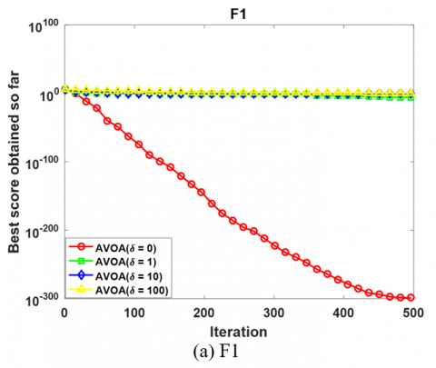
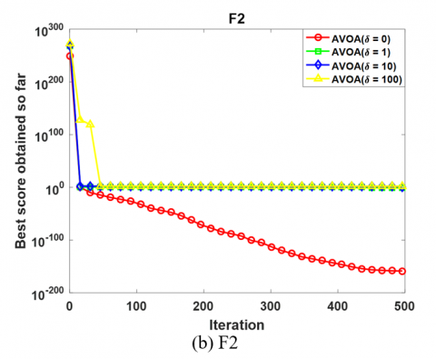
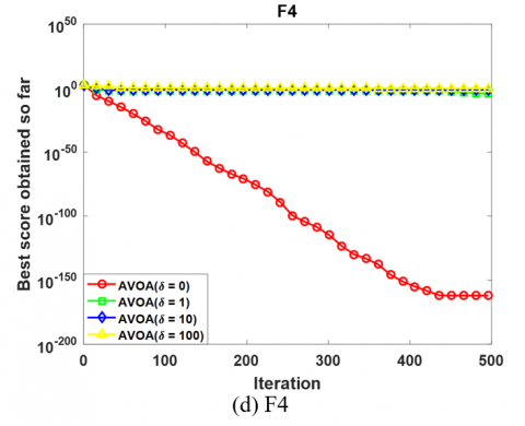
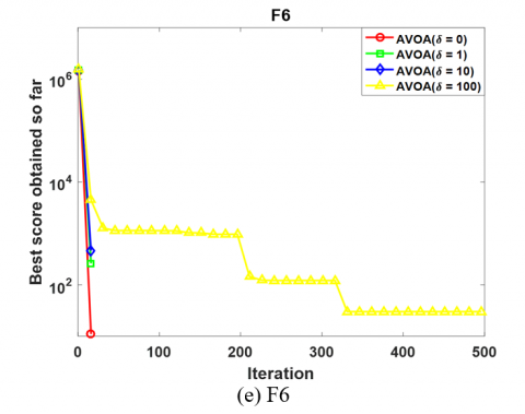
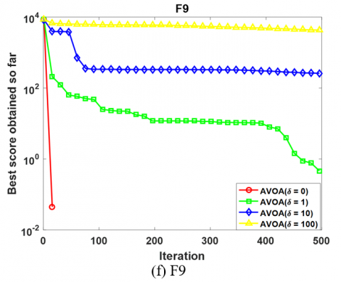
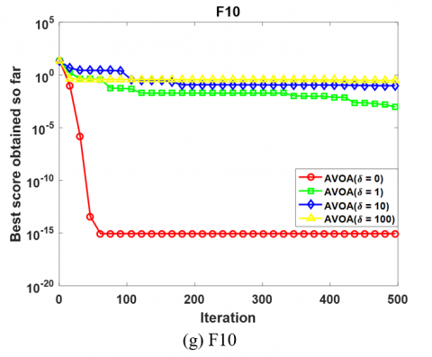
Many papers utilize standard sets of functions to test and validate new algorithms. Within these standard function sets, the AVOA algorithm outperforms commonly used algorithms. However, an interesting phenomenon was discovered in our research: the AVOA algorithm is sensitive to the location of the optimal points of the test functions. If the optimal point of the tested function is at the origin, the AVOA algorithm exhibits significantly better convergence speed and accuracy compared to functions with optimal points not at the origin. To illustrate this phenomenon, we specifically selected test functions F1-F4 and F9-F11, which originally have their optimal points at the origin. To analyze the impact of different optimal points, we introduced an offset represented by δ to these optimal points while maintaining the integrity of the function structures. Additionally, we uniformly shifted the definition ranges of these functions.
Table 1. Definition of offset functions
|
No. |
Function |
Range |
Optimization Value |
Optimal Point |
|
F1 |
f(x)=\sum\limits_{i=1}^{D}{{{({{x}_{i}}-\delta )}^{2}}} |
[-100+δ, 100+δ] |
0 |
(δ, ..., δ) |
|
F2 |
f(x)=\sum\limits_{i=1}^{d}{|}{{x}_{i}}-\delta |+\prod\limits_{i=1}^{d}{|}{{x}_{i}}-\delta | |
[-10+δ, 10+δ] |
0 |
(δ, ..., δ) |
|
F3 |
f(x)=\sum\limits_{i=1}^{D}{(}\sum\limits_{j=1}^{i}{(}{{x}_{j}}-\delta ){{)}^{2}} |
[-100+δ, 100+δ] |
0 |
(δ, ..., δ) |
|
F4 |
f(x)=\underset{1\le i\le D}{\mathop{\max }}\,|{{x}_{i}}-\delta | |
[-100+δ, 100+δ] |
0 |
(δ, ..., δ) |
|
F6 |
f(x)=\sum\limits_{i=1}^{D}{(}\left\lfloor ({{x}_{i}}-\delta )+0.5 \right\rfloor {{)}^{2}} |
[-100+δ, 100+δ] |
0 |
(δ, ..., δ) |
|
F9 |
f(x)=10D+\sum\limits_{i=1}^{D}{\left[ ({{x}_{i}}-\delta )-10\cos (2\pi ({{x}_{i}}-\delta )) \right]} |
[-5.12+δ, 5.12+δ] |
0 |
(δ, ..., δ) |
|
F10 |
f(x)=-20\exp \left( -0.2\sqrt{\frac{1}{D}\sum\limits_{i=1}^{d}{{{({{x}_{i}}-\delta )}^{2}}}} \right)-\exp \left( \frac{1}{D}\sum\limits_{i=1}^{D}{\cos }(2\pi ({{x}_{i}}-\delta )) \right)+20+e |
[-32+δ, 32+δ] |
0 |
(δ, ..., δ) |
|
F11 |
f(x)=\frac{1}{4000}\sum\limits_{i=1}^{D}{{{({{x}_{i}}-\delta )}^{2}}}-\prod\limits_{i=1}^{D}{\cos }\left( \frac{{{x}_{i}}-\delta }{\sqrt{i}} \right)+1 |
[-500+δ, 500+δ] |
0 |
(δ, ..., δ) |
Table 2. Sensitivity analysis of AVOA on 8 offset functions using δ = 0, 1, 10, and 100
|
|
δ = 0 |
δ = 1 |
δ = 10 |
δ = 100 |
|
F1 |
5.53E-319 |
2.69E-07 |
1.95E+00 |
7.71E-01 |
|
F2 |
2.26E-156 |
4.10E-01 |
1.86E+00 |
5.18E+02 |
|
F3 |
4.10E-214 |
5.09E+03 |
1.78E+05 |
2.34E+06 |
|
F4 |
1.54E-162 |
3.90E-05 |
4.38E-02 |
9.81E-01 |
|
F6 |
0.00E+00 |
0.00E+00 |
0.00E+00 |
1.90E+01 |
|
F9 |
0.00E+00 |
5.40E-02 |
5.96E+02 |
3.49E+03 |
|
F10 |
8.88E-16 |
9.41E-04 |
5.89E-01 |
2.36E-01 |
|
F11 |
0.00E+00 |
7.24E-10 |
5.96E-02 |
1.11E+00 |
For detailed expressions of these functions, please refer to Table 1. We conducted tests on the functions listed in Table 1 using the AVOA method with a dimension D of 50 and offset values δ of 0, 1, 10, and 100. The convergence curves of these calculations are displayed in Figure 1, while the corresponding sensitivity analysis data can be found in Table 2. From Figure 1 and Table 2, it can be observed that even if the form of the function remains unchanged, merely changing the position of the optimal point can alter its optimization effect. This phenomenon is inappropriate for an algorithm because, for real-world problems, the position of the optimal solution cannot be known in advance. Therefore, it is necessary to investigate the reasons for this phenomenon and make improvements.
To address this phenomenon, we first conducted an in-depth study of the AVOA algorithm. The original algorithm consists of two stages: exploration and exploitation. During the exploration phase, the algorithm performs random searches to find unutilized or unexplored areas in the function space and generates random noise to escape local optima, providing more useful information for the exploitation phase. In the exploitation phase, the algorithm uses previous probing results and knowledge to accurately identify the global optimal solution, gradually narrowing the search range and rapidly converging to the global optimal solution within the feasible domain.
Figure 1. The convergence curves of AVOA on 8 offset functions using δ = 0, 1, 10, and 100
Therefore, the update formulas during the exploitation phase should be universally applicable and convergent, not just applicable to the origin. To improve the convergence of the optimal point at non-origin locations, in this paper, Eq. (11) and Eq. (14) of the AVOA algorithm are modified to Eqs (18) and (19). From the above formulas, it is evident that even for the optimal point located away from the origin, as the current iteration count t approaches the total iteration count T, the algorithm will be forced to converge towards the optimal point. The term 2×rand-1 is used to introduce randomness and enhance the convergence direction in the iterative algorithm. The new algorithm obtained by updating the two formulas of the existing AVOA algorithm is referred to as EC-AVOA in this paper.
\begin{align} & {{P}_{i,k+1}}={{R}_{i,k}}- {{e}_{k}}\times ({{R}_{i,k}}\times \frac{{{P}_{i,k}}}{2\pi }\times (ran{{d}_{3}}\times \cos ({{P}_{i,k}})+ran{{d}_{4}}\times \sin ({{P}_{i,k}}))) \\\end{align} (18)
\left\{ \begin{array}{*{35}{l}} {{A}_{1}}=B{{V}_{1}}(t)-{{e}_{k}}\times \frac{B{{V}_{1}}(t)\times {{P}_{i,k}}}{B{{V}_{1}}(t)-P_{i,k}^{2}}\times {{S}_{i,k}} \\ {{A}_{2}}=B{{V}_{2}}(t)-{{e}_{k}}\times \frac{B{{V}_{2}}(t)\times {{P}_{i,k}}}{B{{V}_{2}}(t)-P_{i,k}^{2}}\times {{S}_{i,k}} \\\end{array} \right. (19)
{{e}_{k}}=(1-\frac{k}{K})\times (2\times rand-1) (20)
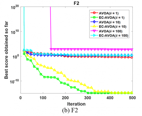
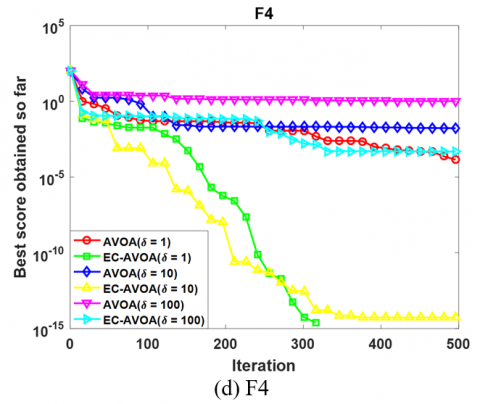
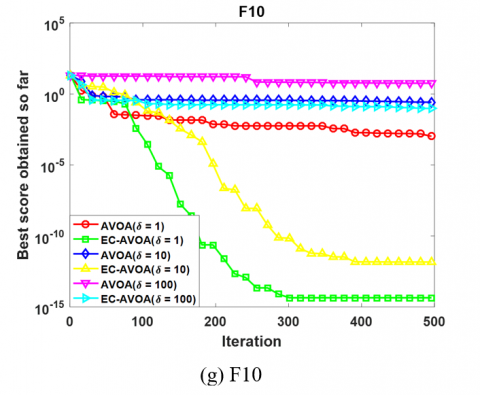
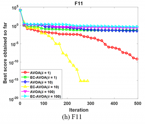
The current study aims to validate that the new algorithm maintains high convergence accuracy even when the optimal solution is not at the origin. To achieve this, we employed the EC-AVOA algorithm to compute eight functions listed in Table 2, with offset values of δ set to 1, 10, and 100, respectively. Subsequently, these computational results were compared with those obtained using the AVOA algorithm. The iterative convergence curves are depicted in Figures 2, with detailed data recorded in Table 3.
Based on the data in Table 3 and Figures 2, the following conclusions can be drawn: as the offset δ increases, the convergence accuracy of the AVOA algorithm significantly decreases. This implies that as the offset increases, the difficulty for these algorithms to find the optimal solution relatively increases. In contrast, the convergence accuracy of the EC-AVOA algorithm also slightly declines, but its performance surpasses that of the original algorithm. The EC-AVOA algorithm maintains relatively stable convergence accuracy under different offsets. It enhances the global convergence and mitigates the impact of the offset by introducing a forced convergence mechanism, thereby improving the performance of the AVOA algorithm. This modification effectively enhances the algorithm's global search capability and robustness, achieving good convergence performance across various offset values. Moreover, except for the F3 function, the EC-AVOA algorithm demonstrates satisfactory convergence performance for both unimodal and multimodal functions.
The algorithm exhibits stability in handling offsets and has been proven to be more suitable and reliable for solving practical problems. In practice, many problem-solving processes involve certain offsets. The EC-AVOA algorithm effectively addresses these offsets and maintains high convergence accuracy, making it a reliable choice for optimizing various practical problems. Whether dealing with unimodal or multimodal functions, the EC-AVOA algorithm shows satisfactory convergence performance, thus serving as a powerful tool for solving complex problems. Therefore, when addressing real-world problems that require consideration of optimal solutions not located at the origin, the EC-AVOA algorithm is trustworthy and worth adopting.
Table 3. Comparison of sensitivity analysis of new algorithms and AVOV on 8 offset functions using δ = 1, 10, and 100
|
|
|
F1 |
F2 |
F3 |
F4 |
F6 |
F9 |
F10 |
F11 |
|
δ=1 |
AVOA |
4.55E-06 |
3.45E-01 |
3.37E+03 |
4.99E-05 |
0.00E+00 |
3.18E-02 |
7.30E-04 |
2.53E-02 |
|
EC-AVOA |
2.86E-08 |
1.44E-15 |
5.86E+02 |
0.00E+00 |
0.00E+00 |
0.00E+00 |
4.44E-15 |
1.54E-08 |
|
|
δ=10 |
AVOA |
3.25E+00 |
2.24E-00 |
9.46E+04 |
1.68E-02 |
0.00E+00 |
3.15E+02 |
2.64E-01 |
8.39E-02 |
|
EC-AVOA |
1.69E-02 |
1.77E-15 |
8.69E+04 |
5.32E-15 |
0.00E+00 |
0.00E+00 |
1.47E-12 |
3.75E-03 |
|
|
δ=100 |
AVOA |
2.16E+01 |
5.78E+02 |
4.48E+06 |
1.01E-01 |
0.00E+00 |
4.45E+03 |
5.72E-00 |
6.09E-03 |
|
EC-AVOA |
1.29E+00 |
2.42E+00 |
1.61E+05 |
4.76E-04 |
0.00E+00 |
9.99E-01 |
9.65E-02 |
2.57E-01 |
Figure 2. The convergence curves of new algorithms and AVOV on 8 offset functions using δ = 0, 1, 10, and 100
In this study, a signal of length 2048 was employed as the target for decomposition. The experimental settings included 15 iterations, an initial population size of 10, a penalty factor α range of [200, 3500], and a decomposition mode number K range of [2, 10]. The time-domain waveform of the signal is illustrated in Figure 3.
Table 4 presents the optimized VMD parameters obtained using three distinct algorithms: AVOA, MPA, and EC-AVOA. The corresponding iteration curves are depicted in Figure 4.
Figure 3. Time domain waveform of the signal
Table 4. Optimization results of VMD parameters by different algorithms
|
Algorithm |
Optimal Parameters |
Time (s) |
|
|
\alpha |
K |
||
|
AVOA |
223 |
8 |
352 |
|
MPA |
213 |
10 |
729 |
|
EC-AVOA |
239 |
8 |
406 |
As shown in Table 4, the optimization of VMD parameters using AVOA, MPA, and EC-AVOA algorithms resulted in different optimal parameter combinations. Specifically, AVOA yielded α=223 and K=8, MPA resulted in α=213 and K=10, while EC-AVOA achieved α=239 and K=8. Additionally, there were notable differences in computation time among the algorithms: AVOA required 352 seconds, MPA took 729 seconds, and EC-AVOA completed in 406 seconds.
The iteration curves in Figure 4 demonstrate that the EC-AVOA algorithm exhibited the highest convergence efficiency and precision throughout the iterative process. In contrast, AVOA showed the lowest convergence precision, while MPA, although achieving comparable convergence precision to EC-AVOA, had a lower convergence efficiency.
Overall, EC-AVOA demonstrated the best overall performance in optimizing VMD parameters. It not only matched the convergence precision of MPA but also significantly outperformed MPA in terms of computation time, while avoiding the low-precision issues associated with AVOA. Therefore, EC-AVOA provides a more efficient and accurate solution for complex signal decomposition tasks.
Figure 4. Convergence profile of parameter optimised VMDs
This study presents an enhanced VMD method based on EC-AVOV for the decomposition of complex signals. By introducing an EC strategy, the applicability and convergence performance of the traditional AVOV in complex function optimization were significantly improved. Experimental results demonstrate that the EC-AVOV algorithm exhibits higher convergence accuracy and stability when optimizing key VMD parameters, including the number of modes and penalty factors. Notably, the algorithm effectively avoids local optima when dealing with complex functions featuring non-zero offsets. Compared to the original AVOV algorithm, EC-AVOV shows substantial enhancements in global search capability and robustness, displaying good adaptability and convergence effects in the optimization of both unimodal and multimodal functions. Additionally, the EC-AVOV algorithm excels in computational efficiency, significantly outperforming existing optimization algorithms such as MPA and AVOV. This makes EC-AVOV more advantageous in addressing practical engineering problems, providing a more efficient and accurate solution for complex signal decomposition tasks. Future research will further explore the application potential of the EC-AVOV algorithm in multi-objective optimization and algorithm fusion, aiming to expand its scope of application in the field of signal processing.
[1] Dragomiretskiy, K., Zosso, D. (2013). Variational mode decomposition. IEEE Transactions on Signal Processing, 62(3): 531-544. https://doi.org/10.1109/TSP.2013.2288675
[2] Liu, Y., Yang, G., Li, M., Yin, H. (2016). Variational mode decomposition denoising combined the detrended fluctuation analysis. Signal Processing, 125: 349-364. https://doi.org/10.1016/j.sigpro.2016.02.011
[3] Lahmiri, S. (2014). Comparative study of ECG signal denoising by wavelet thresholding in empirical and variational mode decomposition domains. Healthcare technology letters, 1(3): 104-109. https://doi.org/10.1049/htl.2014.0073
[4] Huo, J., Liu, N., Xu, Z., Wang, X., Gao, J. (2024). Seismic facies classification using label-integrated and VMD-augmented transformer. IEEE Transactions on Geoscience and Remote Sensing, 62: 5931010. https://doi.org/10.1109/TGRS.2024.3476285
[5] Zhang, S., Niu, D., Zhou, Z., Duan, Y., Chen, J., Yang, G. (2024). Prediction method of direct normal irradiance for solar thermal power plants based on VMD-WOA-DELM. IEEE Transactions on Applied Superconductivity, 34(8):9002904. https://doi.org/10.1109/TASC.2024.3465370
[6] Al Janabi, M.A. (2021). Multivariate portfolio optimization under illiquid market prospects: A review of theoretical algorithms and practical techniques for liquidity risk management. Journal of Modelling in Management, 16(1): 288-309. https://doi.org/10.1108/JM2-07-2019-0178
[7] Ma, Z., Yang, X., Li, H. (2022). Intelligent supply chain and logistics route optimization algorithm in wireless sensor network. Computational Intelligence and Neuroscience, 2022(1): 8161820. https://doi.org/10.1155/2022/8161820
[8] Küster, T., Rayling, P., Wiersig, R., Pozo Pardo, F.D. (2021). Multi-objective optimization of energy-efficient production schedules using genetic algorithms. Optimization and Engineering, 24,. 447-468. https://doi.org/10.1007/s11081-021-09691-3
[9] Penghui, L., Ewees, A.A., Beyaztas, B.H., Qi, C., et al. (2020). Metaheuristic optimization algorithms hybridized with artificial intelligence model for soil temperature prediction: Novel model. IEEE Access, 8: 51884-51904. https://doi.org/10.1109/ACCESS.2020.2979822
[10] Holland, J.H. (1992). Adaptation in Natural and Artificial Systems: An Introductory Analysis with Applications to Biology, Control, and Artificial Intelligence. MIT Press.
[11] Mahfoud, S.W. (1992). A genetic algorithm for parallel simulated annealing. Parallel Problem Solving from Nature, 2: 301-310.
[12] Faramarzi, A., Heidarinejad, M., Mirjalili, S., Gandomi, A.H. (2020). Marine Predators Algorithm: A nature-inspired metaheuristic. Expert Systems with Applications, 152: 113377. https://doi.org/10.1016/j.eswa.2020.113377
[13] Shaheen, M.A., Yousri, D., Fathy, A., Hasanien, H.M., Alkuhayli, A., Muyeen, S.M. (2020). A novel application of improved marine predators algorithm and particle swarm optimization for solving the ORPD problem. Energies, 13(21): 5679. https://doi.org/10.3390/en13215679
[14] Mirjalili, S., Mirjalili, S.M., Lewis, A. (2014). Grey wolf optimizer. Advances in Engineering Software, 69: 46-61. https://doi.org/10.1016/j.advengsoft.2013.12.007
[15] Too, J., Abdullah, A. R., Mohd Saad, N., Mohd Ali, N., Tee, W. (2018). A new competitive binary grey wolf optimizer to solve the feature selection problem in EMG signals classification. Computers, 7(4): 58. https://doi.org/10.3390/computers7040058
[16] Xue, J., Shen, B. (2020). A novel swarm intelligence optimization approach: sparrow search algorithm. Systems Science & Control Engineering, 8(1): 22-34. https://doi.org/10.1080/21642583.2019.1708830
[17] Liu, G., Shu, C., Liang, Z., Peng, B., Cheng, L. (2021). A modified sparrow search algorithm with application in 3D route planning for UAV. Sensors, 21(4): 1224. https://doi.org/10.3390/s21041224
[18] Mirjalili, S., Lewis, A. (2016). The whale optimization algorithm. Advances in Engineering Software, 95: 51-67. https://doi.org/10.1016/j.advengsoft.2016.01.008
[19] Abdollahzadeh, B., Gharehchopogh, F.S., Mirjalili, S. (2021). African vultures optimization algorithm: A new nature-inspired metaheuristic algorithm for global optimization problems. Computers & Industrial Engineering, 158: 107408. https://doi.org/10.1016/j.cie.2021.107408
[20] Zhang, J., Khayatnezhad, M., Ghadimi, N. (2022). Optimal model evaluation of the proton-exchange membrane fuel cells based on deep learning and modified African Vulture Optimization Algorithm. Energy Sources, Part A: Recovery, Utilization, and Environmental Effects, 44(1): 287-305. https://doi.org/10.1080/15567036.2022.2043956
[21] Gürses, D., Mehta, P., Sait, S.M., Yildiz, A.R. (2022). African vultures optimization algorithm for optimization of shell and tube heat exchangers. Materials Testing, 64(8): 1234-1241. https://doi.org/10.1515/mt-2022-0050
[22] Kumar, C., Mary, D.M. (2021). Parameter estimation of three-diode solar photovoltaic model using an Improved-African Vultures optimization algorithm with Newton–Raphson method. Journal of Computational Electronics, 20: 2563-2593. https://doi.org/10.1007/s10825-021-01812-6
[23] Khodadadi, N., Soleimanian Gharehchopogh, F., Mirjalili, S. (2022). MOAVOA: a new multi-objective artificial vultures optimization algorithm. Neural Computing and Applications, 34(23): 20791-20829. https://doi.org/10.1007/s00521-022-07557-y
[24] Balakrishnan, K., Dhanalakshmi, R., Seetharaman, G. (2022). S-shaped and V-shaped binary African vulture optimization algorithm for feature selection. Expert Systems, 39(10): e13079. https://doi.org/10.1111/exsy.13079
[25] Xiao, Y., Guo, Y., Cui, H., Wang, Y., Li, J., Zhang, Y. (2022). IHAOAVOA: An improved hybrid aquila optimizer and African vultures optimization algorithm for global optimization problems. Mathematical Biosciences and Engineering, 19(11): 10963-11017. https://doi.org/10.3934/mbe.2022512
[26] Liu, R., Wang, T., Zhou, J., Hao, X., Xu, Y., Qiu, J. (2022). Improved African vulture optimization algorithm based on quasi-oppositional differential evolution operator. IEEE Access, 10: 95197-95218. https://doi.org/10.1109/ACCESS.2022.3203813