Yang Gao![]() | Zhenxu Wang*
| Zhenxu Wang*![]() | Honggang Luan
| Honggang Luan![]() | Zengfeng Song
| Zengfeng Song![]() | Chuanxi Zhang
| Chuanxi Zhang![]() | Jingshuai Yang
| Jingshuai Yang![]()
© 2024 The authors. This article is published by IIETA and is licensed under the CC BY 4.0 license (http://creativecommons.org/licenses/by/4.0/).
OPEN ACCESS
Object detection in point clouds serves as an important foundation for many applications such as autonomous driving and roadside perception. The existing methods for this foundation can be roughly divided into two categories, which are one-stage methods and multi-stage methods. For the one-stage method, an improved Pointpillars neural network, called MSCS-Pointpillars, was proposed to detect objects directly from point clouds. Here, an attention mechanism and pillars of different scales for the Pointpillars network were introduced to solve the problem of information loss caused by single scale pillar partition. For the multi-stage method, a flexible multi-stage algorithm AF3D, where point clouds were first clustered into clusters which were then detected by a much simpler classifier based on deep learning, was proposed. The two methods on both KITTI dataset and our own dataset have been compared. The results show that MSCS-Pointpillars exhibits better accuracy, but it is difficult to maintain its good performance in unfamiliar scenes. For AF3D, the accuracy appears worse, but it demonstrates much better robustness to unfamiliar scenes.
autonomous vehicles, 3D object detection, deep learning, point clouds, MSCS-Pointpillars
The development of Intelligent Connected Vehicle (ICV) and Cooperative Vehicle Infrastructure System (CVIS) is expected to greatly improve the safety and the efficiency of our traffic system [1]. Among many related technologies, environmental perception plays a very important and fundamental role for both ICV and CVIS. Benefit from its strong environmental adaptability and the capability to acquire accurate distance information, LiDAR has become one of the most popular sensors for the perception task [2, 3]. Quite different from camera, which is arguably the most popular sensor in this field, LiDAR provides 3D point clouds rather than 2D image. So, detecting objects from 3D point clouds is becoming an important research.
Traditional approaches for the recognition task in 3D points cloud generally adopt a multi-stage frame, which clusters the points and then recognizes the clusters. On the other hand, many cutting-edge researches proposed a one-stage frame, which employs deep learning technology to recognize objects in an end-to-end manner [4]. One-stage methods are generally more accurate, while needing a very complex classifier. On the other hand, multi-stage methods generally generate proposals in the first stage, and then recognize objects in the second stage. For the proposal generation stage, they mostly generate proposals through methods, such as sliding window method, anchor-based method, etc. For the recognizing objects stage, pattern match technology and deep learning technology are widely used.
Although one-stage methods have shown great accuracy on performance, they greatly rely on the quality of sample data and show quite different characteristics compared with the multi-stage methods. So in this paper, the performance of the two different frames using two algorithms, namely MSCS-Pointpillars and AF3D, was compared.
For the one-stage method, MSCS-Pointpillars (Multi-Scale Channel Spatial Attention Pointpillars) method was proposed, which reduces the information loss, based on the Pointpillars method. For the multi-stage methods, a flexible multi-stage 3D point clouds object detection method AF3D (Accurate and Flexible 3D Object Detection Algorithm) was proposed, where the points are first clustered and then detected by a neural network.
The rest of the paper is organized as follows. Section 2 briefly reviews relevant research about 3D object detection, which will be the basis for our later work. Section 3 introduces the details of our methods and the verification on the KITTI 3D Object dataset. In section 4, the experiments on our vehicle were described and the character of the two frames of detection based on the experiment results was discussed. Concluding the paper and propose the future work in Section 5.
2.1 End to end frame methods
Deep learning-based methods generally adopt end-to-end frames, which can be divided into two categories according to the input form of points. The two categories include methods based on structured grid and methods based on raw point clouds. The first category of methods generally feeds the deep learning network different types of grid representation while the latter category feeds the raw points directly. These grid representations generally include voxel methods, multi-view projection image and higher dimensional lattices.
The methods based on structured grid are generally efficient while they inevitably lose information. The detection methods based on raw points can retain more details, while they generally consume more computation resources.
2.1.1 Grid-based methods
Typical grid-based methods may first map 3D point clouds into voxel space, and then use 3D convolution or sparse convolution for feature extraction. The classical models include VoxelNet [5], SECOND [6], Pointpillars [7], etc. Zhou and Tuzel [5] proposed the VoxelNet algorithm, which divides the raw point clouds into several voxel grids, uses VFE (Voxel Feature Encoding) layer for local point clouds feature extraction, and 3D convolution to obtains global features while a RPN (Region Proposal Network) is used to detect and locate the objects. Y. Yan etc. [6] improved the VoxelNet and proposed a spatially sparse convolutional network called SECOND which reduced the consumption of computation resources and improved the training speed. Lang et al. [7] proposed a very efficient algorithm called Pointpillars, which divides the point clouds into a certain number of pillars, and then converts them into pseudo-images [8]. However, Pointpillars compresses the raw points into single scale pillar division, which may still cause information loss.
Some other methods project the original point clouds into an aerial view or a frontal view, so that the unordered point clouds in 3D space would be converted into a regular image, which is more convenient to apply image recognition algorithms like Yolo, CNN etc. The classical models of this type include YOLO3D [9], Complex-YOLO [10], etc.
2.1.2 Raw point clouds-based methods
Classic raw point clouds-based detection methods include Pointnet [11], Pointnet++ [12], 3D-SSD [13], Point-GNN [14], SPG [15], etc. In 2017, Qi et al. [11] proposed Pointnet, which directly feeds a deep learning network with raw point clouds. Then Pointnet extracts features from point clouds through a number of shared MLPs, and performs maximum pooling in each dimension of the feature map to obtain global features. Paigwar et al. [16] improved Pointnet with a visual attention mechanism. Qi et al. [12] proposed an improved version called Pointnet++, which presented a hierarchical feature learning architecture for better abstraction of multi-scale features. Yang et al. [13] proposed 3D-SSD algorithm which uses a feature distance-based farthest point sampling method to exclude background points, while semantic information has also been considered. In 2021, Xu et al. [15] proposed a so-called SPG method, which generates semantic point sets and then merges them with the original point clouds to obtain an enhanced point clouds. After that, a point clouds detector is employed to obtain the detection results.
2.2 Multistep frame methods
Multistep frame methods generally include a points extraction or cluster step before the recognizing step. Common clustering methods include five categories, that are partition clustering, distance clustering, density clustering, hierarchical clustering and grid clustering [17]. K-means clustering algorithm may be one of the most typical partition clustering algorithms, which iteratively finds the centers of different clusters and the points nearest to the centers respectively. However, K-means algorithm requires too many manually-adjusted parameters and performs poorly regarding complex shape objects. Recent progress of the partition clustering algorithm may be found in the study [18]. Euclidean clustering may be one of the most typical distance clustering algorithms, which clusters the nearest points into one class. As a very typical density cluster algorithm, DBSCAN (Density-Based Spatial Clustering of Applications with Noise) treats the closely-linked points as one cluster. Some recent progress of this category may be found in the studies [19, 20]. In recent years, hybrid clustering algorithms, which combine several different cluster algorithms, have gradually attracted more attention. Wang et al. [21] proposed the SPSO-FCM algorithm which combines the improved particle swarm optimization algorithm with the fuzzy C-means algorithm to cluster the points. The algorithm has fast convergence speed and clear boundary region segmentation. For scenes with complex profile and large number of point clouds, it can get better segmentation results. There will be more hybrid clustering algorithms in the future.
For detection, traditional methods have developed various algorithms based on the 3D geometric features of the points. Tan [22] has selected the outer contour and the reflection intensity of the cluster to build a feature vector. Using that feature vector, SVM (Support Vector Machine) has then been employed to detect the cluster. This algorithm has obtained good accuracy at the cost of efficiency. Yang [23] has clustered the point clouds based on the spatial scale, reflection intensity, overall distribution and other geometrical characteristics. Then the clusters were classified by SVM as well. In 2019, Shi et al. [24] migrated the image segmentation network RCNN to point clouds data and proposed a multi-stage 3D object detection network called Point RCNN. The author has further proposed an improved version called PV-RCNN [25] which uses efficient 3D voxel convolution and point clouds convolution to estimate the confidence and spatial location of objects. In 2021, Li et al. [26] proposed an efficient multi-stage detection network LiDAR-RCNN. This method uses a voxelization method to remove background points, and then builds a Pointnet-based network to extract features, classify the object and locate it.
3.1 MSCS-Pointpillars
3.1.1 Pointpillars
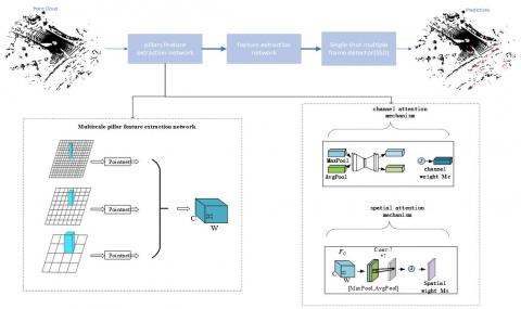
As a popular 3D point clouds detection method, Pointpillars [6] algorithm is composed of several modules that includes: pillars feature extraction module, feature extraction module and single shot multiple frame detection module. In order, an improved Pointpillars called MSCS-Pointpillars, which employs a multi-scale pillars module and an attention mechanism to enhance its ability to detect objects in different sizes was proposed. As shown in Figure 1, the original single-scale pillars with three different scales pillars in the pillars feature extraction module was replaced, and the attention mechanism has been applied.
Figure 1. Overview of MSCS-Pointpillars network
Figure 2. Multiscale pillar feature extraction module of MSCS-Pointpillars, there are three sizes of pillars
Figure 3. Attention module
3.1.2 Multiscale pillars feature extraction network
As shown in Figure 2, 3D laser point clouds data is divided into three pillars of different scales according to the $X Y$-plane where it is located (without considering the $Z$ axis). Beside the basic scale $(H, W)$ proposed by Pointpillars, another two scales of pillars which are $(H / 2, W / 2)$ and $(2 H, 2 W)$ in addition were induced. As a result, three different scales feature maps would be obtained respectively whose size are $(C, 2 H, 2 W),(C, H, W)$, and $(C, H / 2, W / 2)$ respectively. By applying a convolution operation, the feature map whose size is ( $C, 2 H, 2 W$ ) would be compressed to a smaller image whose size is $(C / 2, H, W)$. Similarly, the feature map whose size is $(C, H, W$ ) would be transformed to a smaller size $(C / 2, H, W)$ while the feature map whose size is $(C, H / 2, W / 2)$ would be transformed to $(C / 2, H, W)$. After that, the three different feature maps with three scales would be fused in the channel direction. So that the size of the fused feature map would be $(3 C / 2, H, W)$. After that the fused feature map is further convolved to a smaller feature map $F$, whose size is $(C, H, W)$.
3.1.3 Improved feature extraction based on attention module
As shown in Figure 3, introduce a CBAM (Convolutional Block Attention Module) to improve the detection effect of the network. This makes the network pay more attention on the important information helpful for recognition task. Firstly, apply global max-pooling and average-pooling operations on the feature map $F$ obtained by the multi-scale pillar feature extraction module. The pooling results are then subjected to a matrix add operation after MLP to generate the channel weight $M_C \in R^{C * 1 * 1}$. Then $M_C \in R^{C * 1 * 1}$ are multiplied to the fused feature map $F$ to obtain a channel attention feature map $F_C$. Secondly, $F_C$ is subjected to global max-pooling and average-pooling operations by the channel as well. The pooling results are spliced and then subjected to a $7 * 7$ convolution operation to generate another spatial weight $M_S \in R^{1 * H * W}$. Then the spatial weights $M_S \in R^{1 * H * W}$ and $F_C$ are multiplied to obtain a weighted feature map $F_{C S}$ with channel spatial weight information, and then $F_{C S}$ is sent to the feature extraction network for higher level representations. Specifically, it involves feature extraction of feature maps through two-dimensional convolution.
3.1.4 Loss function
The output of the MSCS-Pointpillars network mainly includes the category of the object and the parameters of the $3 \mathrm{D}$ bounding box. The $3 \mathrm{D}$ bounding box can be represented by parameters $(x, y, z, w, l, h, \theta)$, where $(x, y, z)$ represents the coordinates of the center of the $3 \mathrm{D}$ bounding box. $(w, l, h)$ represents the width, length, and height of the $3 \mathrm{D}$ bounding box respectively. $\theta$ represents the rotation angle around the $Z$-axis (the $Z$-axis is the axis perpendicular to the ground). So, the loss function is designed as shown in Eq. (1), which includes $3 \mathrm{D}$ bounding box regression loss, classification loss, orientation loss.
$\ell=\frac{1}{N_{ {pos }}}\left(\beta_{l o c} \ell_{l o c}+\beta_{c l s} \ell_{c l s}+\beta_{d i r} \ell_{d i r}\right)$ (1)
where, $N_{\text {pos }}$ represents the number of positive samples generated boxes, $\ell_{\text {loc }}$ represents the $3 \mathrm{D}$ box regression loss function, $\ell_{c l s}$ represents the classification loss function, and $\ell_{d i r}$ represents the object orientation loss function. $\beta_{l o c}, \beta_{c l s}$, $\beta_{d i r}$ are the corresponding weights. In this paper, use the loss function parameters of Pointpillars network for reference, and set $\beta_{l o c}=2, \beta_{c l s}=2, \beta_{d i r}=2$.
The $3 \mathrm{D}$ bounding box regression loss function is shown in Eq. (2), which mainly includes the $3 \mathrm{D}$ box position regression loss, the size regression loss and the orientation regression loss, as shown in Eqs. (3), (4) and (5) respectively.
$\ell_{l o c}=\sum_{b \in(x, y, z, w, l, h, \theta)} \operatorname{Smooth}_{L 1}(\Delta b)$ (2)
$\Delta x=\frac{x_{g t}-x_p}{d_p}, \Delta y=\frac{y_{g t}-y_p}{d_p}, \Delta z=\frac{z_{g t}-z_p}{d_p}$ (3)
$\Delta w=\log \frac{w_{g t}}{w_p}, \Delta l=\log \frac{l_{g t}}{l_p}, \Delta h=\log \frac{h_{g t}}{h_p}$ (4)
$\Delta \theta=\sin \left(\theta_{g t}-\theta_p\right)$ (5)
$d_p=\sqrt{w_p^2+l_p^2}$ (6)
where, $x_{g t}, y_{g t}, z_{g t}, w_{g t}, l_{g t}, h_{g t}, \theta_{g t}$ represent the truth value. The $x_p, y_p, z_p, w_p, l_p, h_p, \theta_p$ represent the predicted value by the network.
The classification loss $\ell_{c l s}$ is shown in Eq. (7):
$\ell_{c l s}=-\alpha_a\left(1-p^a\right)^\gamma \log _p \alpha$ (7)
where, $p^a$ represents the possibility of a certain category. According to reference paper Lang et al. [7], set $\alpha$ to 0.25 , and $\gamma$ to 2 .
Since Eq. (5) cannot distinguish the $3 \mathrm{D}$ box flipping $0^{\circ}$ and $180^{\circ}, \ell_{\text {dir }}$ uses the Softmax function to learn the orientation of the 3D bounding box in discrete directions [6].
3.2 AF3D
Our work combined traditional object detection algorithms and built a PFC-Net network based on Pointnet, proposing a flexible and accurate 3D object detection algorithm AF3D. The AF3D algorithm framework is shown in Figure 4. The entire algorithm framework mainly consists of two stages. In the first stage, ground segmentation is performed first, and then the remaining point clouds are clustered to obtain point clouds clusters $\left\{C_1, C_2, C_3, \cdots, C_{k-1}, C_k\right\}$. In the second stage, the point clouds classification network PFC-Net is first built. Secondly, clusters are inputted into the trained classification network PFC-Net to classify the clusters. Subsequently, obtain the semantic information of each cluster class, perform bounding box fitting on the classified objects, and obtain network inference results.
Figure 4. AF3D network overview
3.2.1 Stage 1: Ground point clouds segmentation and non-ground point clouds clustering
A segmentation fitting algorithm proposed by Zermas et al. [27] to extract and remove the ground points was employed. After that, the non-ground point clouds were segmented and clustered using DBSCAN algorithm.
For the DBSCAN algorithm, the clustering neighborhood radius (Eps) was set to 0.45 meters, the Euclidean distance metric was adopted, and the minimum number of points required for a core point (MinPts) was set to 10. The non-ground point clouds clustering effect obtained by using DBSCAN is shown in Figure 5. The first column shows the point clouds clustering effect, and the second shows the original images accordingly. It was found that all the point clouds are properly clustered.
3.2.2 Stage 2: Point clouds Classification Network PFC-Net
Because point clouds have been clustered, a very simple classification network named PFC-Net to classify each cluster was designed. The network structure of PFC-Net is shown in Figure 6. The clusters were inputted as a tensor with size $(N, 3)$, where $N$ represents the number of points inputted and 3 represents the channel information of each point. Feature extraction is performed by a multiple weight-shared MLP modules. So that a feature map $F_1$ represented by a tensor with size $(N, 1024)$ is obtained. After that, a global feature map, with size $(1,1024)$, is obtained by a Max-Pooling layer. By concatenating both the global feature and the feature map $F_1$, a feature map $F_2$, which is represented by a tensor with size $(N, 2048)$, is obtained. $F_2$ contains both the detailed features and the global features of the cluster. The feature map $F_2$ is then passed through two weight-shared MLPs and a MaxPooling layer for further feature extraction to form a new feature map $F_3$ represented by a tensor whose size is $(1,1024)$. After that $F_3$ is sent to three fully connected layers for classification result.
Figure 5. Point clouds clustering results based on DBSCAN algorithm
Figure 6. The structure of the point clouds classification network PFC-Net: it takes N points as input, and output the classification scores for 4 classes, namely pedestrian, car, cyclist and other object
3.2.3 PFC-Net network training
1) KITTI 3D Object Dataset
Here KITTI 3D Object dataset was used to train PFC-Net and to test its performance. As one of the most commonly used public dataset, KITTI 3D Object dataset [28] was chosen to verify the performance of PFC-Net network. KITTI 3D Object dataset consists of 7481 training samples and 7518 testing samples, mainly including various types of cars, pedestrians, and cyclists. The KITTI 3D Object dataset covers multiple scenes such as highways, suburbs, and urban roads. Each frame of data includes both point clouds and their corresponding RGB images, label files, etc. According to the cutoff value and the occlusion scale, the dataset samples can be categorized into easy, medium and difficult levels, which also represent the difficulty of detection as shown in Table 1.
2) Dataset reconstruction
The original KITTI 3D Object dataset contains point clouds of the whole scene rather than the clusters, which cannot be directly used for PFC-Net. Therefore, the KITTI 3D Object dataset was reconstructed. First, according to the label files, the point clouds data belonging to three categories, namely cars, cyclists, and pedestrians, is extracted. Second-ly, the data augmentation method to balance the number of samples in each category for better training effect was used. The specific steps are as follows:
a) Object point clouds extraction
For each frame of point clouds in the KITTI training set, the label categories of “Van”, “Car”, “Truck”, and “Tram” are unified into “Car”. So that only "Car", "Pedestrian", "Cyclist" are kept. Figure 7 (a) and (b) show an extraction example where a pedestrian denoted by green points has been extracted from the original points clouds. The visualization results of the extracted clusters belonging to the three categories are shown in Figure 8 (a), (b) and (c) respectively. In addition, due to the characteristics of lidar, the spatial information of objects may seriously be missing due to too sparse points. Therefore, three threshold values for the number of points belonging to the category of "Car", the "Pedestrian", the "Cyclist" that are 200, 50, 50 were stipulated respectively.
Table 1. KITTI dataset object detection level division
|
Level |
Easy |
Medium |
Difficult |
|
degree of occlusion |
Fully visible |
partially visible |
Hardly visible |
|
cutoff value |
$\leq$ 15% |
15%~50% |
$\geq$ 50% |
|
number of pixels |
$\geq$ 40 |
$\geq$ 25 |
|
Figure 7. Object point clouds extraction process
Figure 8. Visualization results of point clouds extraction for each category of KITTI dataset
b) Data augmentation
After object points extraction, the amount of "Car", "Pedestrian", "Cyclist" categories are 12564, 3272, 1526 respectively. It can be found that the proportions of the three types in the samples are imbalanced, thus making training for the category insufficient due to imbalanced proportions, and impacting the classification accuracy.
Therefore, apply data augmentation to the categories with small proportion in training set. The samples in the categories with small proportion were translated and randomly rotated angle around the $Z$-axis of the lidar coordinate system. On the other hand, the Weighted Random Sampler method, which selects training data based on the weight of each category was also used, to solve the problem of imbalanced sample proportions. The proportion of samples after data augmentation and weighted random sampling is shown in Table 2.
According to the study [29], only objects located within 40m ahead, would be properly detected when the speed of the car reaches 80 Km/h. So only obstacles located in that range would be classified by the algorithms in the following verification.
Table 2. The proportion of each category before and after data augmentation (%)
|
Category |
Car |
Pedestrian |
Cyclist |
Other Objects |
|
Before data augmentation |
46.92 |
13.41 |
5.24 |
44.91 |
|
After data augmentation |
37.45 |
23.67 |
18.33 |
20.55 |
|
After weighted random sampling |
25.46 |
24.67 |
24.36 |
25.51 |
3) Verification of PFC-Net
The verification was running on a workstation equipped with Intel i7 10700KF and NVIDIA RTX 3080 graphics card. The software environment includes Ubuntu 18.04 LTS, CUDA 11.1, cuDNN 8.0.5, and Python 3.7.
If the number of the inputted points is less than 1024, it will be augmented to 1024 using zero padding. If the number of the inputted points is bigger than 1024, it will be down sampled to 1024 using farthest points sampling technique.
The reconstructed KITTI 3D Object dataset is divided into training set and test set according to the ratio of 8:2. The cross-entropy loss function shown as Eq. (8) was adopted for PFC-Net.
$L=\frac{1}{N} \sum_i L_i=-\frac{1}{N} \sum_i \sum_{c=1}^M y_{i c} \log \left(p_{i c}\right)$ (8)
where, $M$ represents the number of categories, $i$ is the sample index, $c$ is the category index and $y_{i c}$ represents a sign function where $y_{i c}$ equal to 1 only if the predicted category of the network is consistent with the label, other wise $y_{i c}$ equal to $0 . p_{i c}$ represents the predicted confidence of the sample $i$ belonging to the category $c$.
The Adam (Adaptive Moment Estimation) optimizer with an initial learning rate of $1 * 10^{-3}$ is adopted, while the learning rate is attenuated by 0.8 times every 15 cycles. The epoch is set to 150, while the batch size is set to 128.
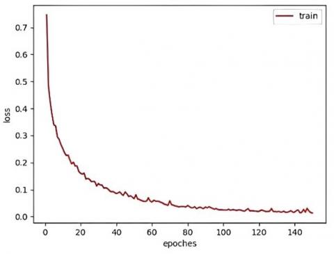
Figure 9. PFC-Net training loss curve: the vertical axis represents the loss function value, and the horizontal axis represents the number of training epochs
The training loss curve of PFC-Net is shown in Figure 9, where the vertical axis represents the loss value, and the horizontal axis represents the number of training epochs. It shows that the training mostly fits after the 120th training epoch.
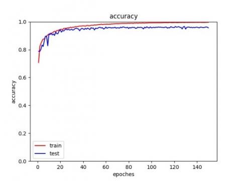
The average accuracy curve is shown in Figure 10, where the vertical axis represents the overall accuracy, and the horizontal axis represents the number of training epochs. The red curve represents the accuracy of classification on the training set. while the blue curve represents the accuracy of classification on the test set. It can be found that after being welltrained, the average accuracy of point clouds classi-fication on the training set is as high as 99.21%, and the average accuracy of point clouds classification on the test set reaches 95.78%.
Figure 10. PFC-Net classification average accuracy curve: the vertical axis represents the overall accuracy, and the horizontal axis represents the number of training cycles
3.3 Verification of two methods on KITTI
3.3.1 Verification of MSCS-Pointpillars
The performance of MSCS-Pointpillars was also verified on the KITTI 3D Object Dataset. According to the practice by Chen et al. [30], redividing the 7481 samples into training and testing set samples, of which the number of training set samples is 3712 and the number of test set samples is 3769.
In the training of MSCS-Pointpillars, the maximum number of epoch iterations is set to 160, Adam optimizer’s initial learning rate is set to $2 * 10^{-4}$, while the learning rate is attenuated by 0.8 times every 15 cycles. The region of interest is intercepted by passthrough filtering, and the values are shown in Eq. (9).
$\left\{\begin{array}{c}0 \leq x \leq 80.64 \\ -40.32 \leq y \leq 40.32 \\ -1<z<3\end{array}\right.$ (9)
The maximum number of pillars, denoted as $P$, is set to 12000, and the maximum number of points in the pillar is set to 100.
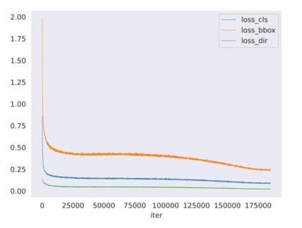
For better comparison, all the samples were classified into easy, medium and hard, according to three overlap thresholds, respectively. For cars, the easy, medium and hard overlap thresholds are set to 0.7, 0.7, 0.7 times IoU, respectively. The overlap thresholds are set to 0.5, 0.5, 0.5 times IoU for the cyclist categories and the pedestrian categories. The training loss curve is shown in Figure 11. In the legend of the figure, “loss_cls” represents the classification loss, “loss_bbox” represents the loss of the 3D box, and loss_dir represents the orientation loss.
Our work uses the average precision as the criteria. The verification results on the KITTI 3D Object data set are shown in Table 3 where the performance is displayed according to different difficulty degrees. It can be found that compared to Pointpillars, MSCS-Pointpillars has been improved on almost all categories.
Figure 11. MSCS-Pointpillars training Loss curve: the vertical axis represents the loss value, and the horizontal axis represents the epochs
Table 3. Comparison with Pointpillars on the KITTI 3D object test set (%)
|
Categories |
Degree |
Pointpillars |
MSCS-Pointpillars |
|
Cars |
Easy |
83.60 |
87.59 |
|
Medium |
74.58 |
78.63 |
|
|
Difficult |
71.55 |
76.47 |
|
|
Pedestrians |
Easy |
50.31 |
53.60 |
|
Medium |
44.08 |
47.71 |
|
|
Difficult |
40.97 |
43.36 |
|
|
Cyclists |
Easy |
79.76 |
81.02 |
|
Medium |
59.35 |
62.49 |
|
|
Difficult |
56.38 |
58.86 |
3.3.2 Verification of AF3D
For the car category, the maximum height is set to 2.5m, the maximum length is set to 8m, and the minimum height threshold is 1.5m. Due to the severe occlusion of some cars in the dataset, the minimum length threshold for car size is not specified. When the height and length of the cluster is greater than the maximum height and length threshold of the car category or when the height of the cluster is less than the minimum height threshold, it can be discarded. For the cyclist category, the maximum height threshold is set to 2m, the maximum length threshold is 2.5m, and the minimum height threshold is 1.25m. For the pedestrian category, the maximum height threshold is set to 2m and the minimum height threshold is 1.25m.
Similarly, the verification results of AF3D on the KITTI 3D Object dataset are shown in Table 4.
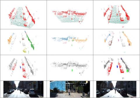
The visualization results of AF3D on KITTI 3D Object dataset are shown in Figure 12.
Figure 12. The visualization results of AF3D on KITTI 3D Object dataset: the first row of images represents the extraction of ground points (ground is shown in green, non-ground point clouds is shown in gray); the second row of images is a visualization of the clustering effect; the third row of images is a classification of the clusters (cars is shown in red, blue for cyclists is shown in blue, and pedestrians is shown in green); the fourth row shows the original RGB image corresponding to the point clouds, respectively
Table 4. Detection accuracy (%) of AF3D algorithm on KITTI 3D object dataset
|
Categories |
Degree |
AF3D |
|
Cars |
Easy |
73.92 |
|
Medium |
70.87 |
|
|
Difficult |
62.41 |
|
|
Pedestrians |
Easy |
43.21 |
|
Medium |
41.52 |
|
|
Difficult |
38.83 |
|
|
Cyclists |
Easy |
68.32 |
|
Medium |
61.76 |
|
|
Difficult |
51.42 |
|
|
Training time (hours) |
5.6 |
|
In this section, the algorithm was run on our own vehicle to conduct an experimental comparison between the MSCS-Pointpillars and AF3D algorithms, then the advantages and disadvantages of the two methods were analyzed comprehensively.
4.1 Experiment platform
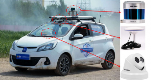
The hardware equipment on the car includes HESAI Technology Pandar 64-line lidar, monocular, camera, RTK GPS and a laptop, as shown in Figure 13.
4.2 Experiment data
Driver drove the experimental car along a road in our campus. Part of the scene is shown in Figure 14. Because the speed of the car is relatively low, point clouds data is captured in every 2s. So that our experiment dataset includes 200 frames of point clouds data. 3D bounding boxes are employed to label cars, cyclists, and pedestrians.
Figure 15 shows some labeling result where red represents cars, green represents pedestrians, and purple represents cyclists.
After trained on KITTI dataset, the MSCS-Pointpillars and AF3D were tested on our experiment dataset neither with retraining nor refining, and the detection accuracy is shown in Table 5.
Figure 13. Experiment platform
Figure 14. Examples of some scenarios in our experiment: the first column shows point clouds, and the second column shows the corresponding RGB image
Figure 15. Point clouds data and the labels
Table 5. The detection accuracy (%) of the two algorithms on our experiment data set
|
Methods |
Cars |
Pedestrians |
Cyclists |
|
MSCS-Pointpillars |
54.39 |
32.88 |
39.23 |
|
AF3D |
69.74 |
41.25 |
54.33 |
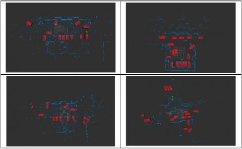
Some examples of the detection results obtained by both AF3D and MSCS-Pointpillars are shown in Figure 16. Here, the first column shows the detection results using AF3D network, and the second column shows the detection results using MSCS-Pointpillars network. The third column shows the label results. It can be found that MSCS-Pointpillars has missed more targets than AF3D, although the MSCS-Pointpillars outperforms AF3D on the KITTI 3D Object Dataset. So AF3D shows more detection capability in an unfamiliar scene like our experiment than MSCS-Pointpillars.
From the verification results on the KITTI 3D Object dataset in Sections 3.3.1 and 3.3.2, it can be seen that both methods have good detection capability and the detection accuracy of cars is higher, followed by the accuracy of cyclists. Pedestrians have obtained the lowest detection accuracy. This is because of two reasons. Pedestrians generally produce least number of points compared with the other two categories with similar distance.
It can also be found that the detection accuracy of MSCS-Pointpillars on the KITTI 3D Object dataset outperforms that of AF3D. Because MSCS-Pointpillars can make use of the context information of the whole point clouds, while AF3D can only use the cluster information for recognition.
The training time and the computation cost of AF3D algorithm are much less than those of MSCS-Pointpillars. This is because in AF3D, only PFC-Net, which is much simpler than MSCS-Pointpillars, needs to be trained and the DBSCAN in AF3D is highly efficient.
Without retraining or refining, our experiment utilizes unfamiliar scenes for both MSCS-Pointpillars and AF3D algorithms. The detection accuracy of MSCS-Pointpillars decreased significantly while in contrast, the detection accuracy of AF3D algorithm only suffered a small decrease. In our experiment, the detection accuracy of AF3D on cars, pedestrians and cyclists is 15.35%, 8.37% and 15.1% higher than that of MSCS-Pointpillars, respectively. This is because AF3D employs a traditional clustering algorithm to cluster the point cloud before recognizing it. Moreover, the clusters for each category would only be slightly changed in different scenes, which makes it much easier to be recognized in an unfamiliar scenario. In contrast, MSCS-Pointpillars greatly relied on the context information of the whole scenario for better accuracy performance, while this context information would be greatly changed in unfamiliar scenes.
Figure 16. Visualization of detection results of AF3D and MSCS-Pointpillars in experiment. The first column shows the detection result of the AF3D, and the second column shows the detection result of MSCS-Pointpillars. The third column is the label result. The red point clouds represents that the targets have been detected, while the black represents non target point clouds
This paper has proposed two different approaches for object detection task in 3D point clouds. MSCS-Pointpillars is a type of Deep learning algorithm that adopts an end-to-end frame to fully utilize context information, resulting high accuracy. AF3D is a combination of Deep learning technology and traditional two-step frame. By comparing the performance of these two algorithms, results found that the traditional two-step frame can help on reducing the computation resource request and enhance the adaptability to unfamiliar scenes. Meanwhile end-to-end frame can propose better detection performance while it requires much more computational resources and greatly relies on the universality of the training sample set. On the other way, the accuracy of the two-step frame algorithm greatly relies on the clustering accuracy, while the high recognition accuracy for each cluster would be comparatively easy to be achieved.
This research is funded by Xi'an Municipal Bureau of Science and Technology (Grant No.: 23ZDCYJSGG0011-2022; 23ZDCYJSGG0024-2022).
[1] Atkins, W. (2016). Research on the impacts of connected and autonomous vehicles (CAVs) on traffic flow. Stage 2: Traffic modelling and analysis technical report.
[2] Zamanakos, G., Tsochatzidis, L., Amanatiadis, A., Pratikakis, I. (2021). A comprehensive survey of LIDAR-based 3D object detection methods with deep learning for autonomous driving. Computers & Graphics, 99: 153-181. https://doi.org/10.1016/j.cag.2021.07.003
[3] Ghasemieh, A., Kashef, R. (2022). 3D object detection for autonomous driving: Methods, models, sensors, data, and challenges. Transportation Engineering, 8: 100115. https://doi.org/10.1016/j.treng.2022.100115
[4] Gupta, A., Anpalagan, A., Guan, L., Khwaja, A.S. (2021). Deep learning for object detection and scene perception in self-driving cars: Survey, challenges, and open issues. Array, 10: 100057. https://doi.org/10.1016/j.array.2021.100057
[5] Zhou, Y., Tuzel, O. (2018). VoxelNet: End-to-end learning for point cloud based 3D object detection. In IEEE/CVF Conference on Computer Vision and Pattern Recognition, Salt Lake City, UT, USA, pp. 4490-4499. https://doi.org/10.1109/CVPR.2018.00472
[6] Yan, Y., Mao, Y., Li, B. (2018). Second: Sparsely embedded convolutional detection. Sensors, 18(10): 3337. https://doi.org/10.3390/s18103337
[7] Lang, A.H., Vora, S., Caesar, H., Zhou, L., Yang, J., Beijbom, O. (2019). Pointpillars: Fast encoders for object detection from point clouds. In IEEE/CVF Conference on Computer Vision and Pattern Recognition (CVPR), Long Beach, California, USA, pp. 12689-12697. https://doi.org/10.1109/CVPR.2019.01298
[8] Wang, B. (2022). Research on key technologies of LiDAR-based 3D environment perception system for autonomous driving. Ph.D. dissertation, Changchun Institute of Optics, Fine Mechanics and Physics, Chinese Academy of Sciences, China. https://doi.org/10.27522/d.cnki.gkcgs.2022.000053
[9] Ali, W., Abdelkarim, S., Zidan, M., Zahran, M., El Sallab, A. (2018). Yolo3d: End-to-end real-time 3d oriented object bounding box detection from lidar point cloud. In European Conference on Computer Vision (ECCV) Workshops, Springer, Cham, pp. 716-728. https://doi.org/10.1007/978-3-030-11015-4_54
[10] Simony, M., Milzy, S., Amendey, K., Gross, H.M. (2018). Complex-yolo: An Euler-region-proposal for real-time 3D object detection on point clouds. In European Conference on Computer Vision (ECCV) Workshops, Springer, Cham, pp. 197-209. https://doi.org/10.1007/978-3-030-11009-3_11
[11] Qi, C.R., Su, H., Mo, K., Guibas, L.J. (2017). Pointnet: Deep learning on point sets for 3D classification and segmentation. In IEEE Conference on Computer Vision and Pattern Recognition (CVPR), Honolulu, HI, USA, pp. 77-85. https://doi.org/10.1109/CVPR.2017.16
[12] Qi, C.R., Yi, L., Su, H., Guibas, L.J. (2017). Pointnet++: Deep hierarchical feature learning on point sets in a metric space. Advances in Neural Information Processing Systems, 30.
[13] Yang, Z., Sun, Y., Liu, S., Jia, J. (2020). 3dssd: Point-based 3d single stage object detector. In IEEE/CVF Conference on Computer Vision and Pattern Recognition, Seattle, WA, USA, pp. 11037-11045. https://doi.org/10.1109/CVPR42600.2020.01105
[14] Shi, W., Rajkumar, R. (2020). Point-GNN: Graph neural network for 3D object detection in a point cloud. In IEEE/CVF Conference on Computer Vision and Pattern Recognition, Seattle, WA, USA, pp. 1708-1716. https://doi.org/10.1109/CVPR42600.2020.00178
[15] Xu, Q., Zhou, Y., Wang, W., Qi, C.R., Anguelov, D. (2021). SPG: Unsupervised domain adaptation for 3D object detection via semantic point generation. In IEEE/CVF International Conference on Computer Vision, Montreal, QC, Canada, pp. 15426-15436. https://doi.org/10.1109/ICCV48922.2021.01516
[16] Paigwar, A., Erkent, O., Wolf, C., Laugier, C. (2019). Attentional pointnet for 3D-object detection in point clouds. In IEEE/CVF Conference on Computer Vision and Pattern Recognition Workshops (CVPRW), Long Beach, CA, USA, pp. 1297-1306. https://doi.org/10.1109/CVPRW.2019.00169
[17] Wang, Z., Li, Q., Zhang, Z., Wang, K., Yang, J. (2021). Research progress of unmanned vehicle point cloud clustering algorithm. World Sci-Tech R & D, 43(3): 274-285. https://doi.org/10.16507/j.issn.1006-6055.2020.12.025
[18] Ikotun, A.M., Almutari, M.S., Ezugwu, A.E. (2021). K-means-based nature-inspired metaheuristic algorithms for automatic data clustering problems: Recent advances and future directions. Applied Sciences, 11(23): 11246. https://doi.org/10.3390/app112311246
[19] Fan, X., Xu, G., Li, W., Wang, Q., Chang, L. (2019). Target segmentation method for three-dimensional LiDAR point cloud based on depth image. Chinese Journal of Lasers, 46(7): 0710002. https://doi.org/10.3788/CJL201946.0710002
[20] Zhang, C., Huang, W., Niu, T., Liu, Z., Li, G., Cao, D. (2023). Review of clustering technology and its application in coordinating vehicle subsystems. Automotive Innovation, 6(1): 89-115. https://doi.org/10.1007/s42154-022-00205-0
[21] Wang, X.H., Wu, L.S., Chen, H.W., Shi, H.L. (2017). Region segmentation of point cloud data based on improved particle swarm optimization fuzzy clustering. Optics and Precision Engineering, 25(4): 1095-1105. https://doi.org/10.3788/OPE.20172504.1095
[22] Tan, Y. (2020). Obstacle detection and identification of unmanned driving based on lidar. M.S. thesis, Jilin University, China. https://doi.org/10.27162/d.cnki.gjlin.2020.004659
[23] Yang, H. (2021). Research on real time target clustering and recognition of LiDAR point cloud for autonomous driving. M.S. thesis, University of Science and Technology of China. https://doi.org/10.27517/d.cnki.gzkju.2021.001473
[24] Shi, S., Wang, X., Li, H. (2019). PointRCNN: 3D object proposal generation and detection from point cloud. In IEEE/CVF Conference on Computer Vision and Pattern Recognition (CVPR), Long Beach, CA, USA, pp. 770-779. https://doi.org/10.1109/CVPR.2019.00086
[25] Shi, S., Guo, C., Jiang, L., Wang, Z., Shi, J., Wang, X., Li, H. (2020). PV-RCNN: Point-Voxel feature set abstraction for 3D object detection. In IEEE/CVF Conference on Computer Vision and Pattern Recognition, Seattle, WA, USA, pp. 10526-10535. https://doi.org/10.1109/CVPR42600.2020.01054
[26] Li, Z., Wang, F., Wang, N. (2021). LiDAR R-CNN: An efficient and universal 3D object detector. In IEEE/CVF Conference on Computer Vision and Pattern Recognition (CVPR), Nashville, TN, USA, pp. 7542-7551. https://doi.org/10.1109/CVPR46437.2021.00746
[27] Zermas, D., Izzat, I., Papanikolopoulos, N. (2017). Fast segmentation of 3D point clouds: A paradigm on LiDAR data for autonomous vehicle applications. In IEEE International Conference on Robotics and Automation (ICRA), Singapore, pp. 5067-5073. https://doi.org/10.1109/ICRA.2017.7989591
[28] Geiger, A., Lenz, P., Urtasun, R. (2012). Are we ready for Autonomous Driving? The KITTI Vision Benchmark Suite. In IEEE Conference on Computer Vision and Pattern Recognition (CVPR), Providence, RI, USA, pp. 3354-3361. https://doi.org/10.1109/CVPR.2012.6248074
[29] Li, B. (2019). On enhancing ground surface detection from sparse lidar point cloud. In IEEE/RSJ International Conference on Intelligent Robots and Systems (IROS), Macau, China, pp. 4524-4529. https://doi.org/10.1109/IROS40897.2019.8968135
[30] Chen, X., Kundu, K., Zhu, Y., Ma, H., Fidler, S., Urtasun, R. (2018). 3D object proposals using stereo imagery for accurate object class detection. IEEE Transactions on Pattern Analysis and Machine Intelligence, 40(5): 1259-1272. https://doi.org/10.1109/TPAMI.2017.2706685