Mojtaba Nasehi![]() | Mohsen Ashourian*
| Mohsen Ashourian*![]() | Hossein Emami
| Hossein Emami![]()
© 2024 The authors. This article is published by IIETA and is licensed under the CC BY 4.0 license (http://creativecommons.org/licenses/by/4.0/).
OPEN ACCESS
Vehicle-type detection tool has many applications in transportation, traffic control, guiding and controlling unmanned vehicles, tolls and road taxes, traffic violations, smuggling detection, etc. In the proposed version, the MobileNet neural network and the YOLO V5 algorithm are integrated. In this integration, the YOLO V5 algorithm replaces the convolutional layers of the neural network and the neural network be used for the classification of vehicles. The Kivy library is employed to transform the developed algorithm into an Android application. The data used in this study consists of two datasets: The ImageNet database and a constructed database. The proposed method results show improvement in increasing the accuracy of vehicle detection, reducing the computational load, detection accuracy in different weather conditions, separating overlapping cars. Various methods are presented for better neural network training and reducing neural network size. The reason for these capabilities is the use of developed algorithms and the use of techniques such as data augmentation, spatial filtering, and distillation.
vehicle type detection, object recognition, MobileNet, neural network, YOLO V5
Today, vehicle-type detection is used in various fields. Its application in transportation, providing traffic permits and road taxes, detecting smuggling, registering traffic violations, controlling unmanned vehicles, and managing smart cities are some of the things that show the importance of vehicle-type detection.
There are limitations to detect vehicles in the image, which are:
• The image processing system needs very detailed images from specific angles of the car.
• Variety in cars, for example, car rides, buses, etc.
• The pictures are taken in different weather conditions and light changes.
In this article, the proposed method is based on the integration of the Mobilenet neural network and YOLO V5 algorithm. For this purpose, the proposed method has been compared with the RFCN method. In the proposed method, the results obtained from simulation are about 98.5%, and the results obtained practically from different environments are about 98%, which are more accurate and efficient than other methods. From another point of view, the hardware implementation of algorithms and solutions is of special importance because there are bottlenecks in the implementation of the scenario in the form of simulation and converting it into hardware. The implementation of the proposed method using the database shows a good performance. The features of the proposed method are: reducing the calculation load, high efficiency, higher detection accuracy, and applicability in different weather conditions.
The next chapters of the paper are organized as follows. Chapter 2 presents related works, Chapter 3 introduces the proposed method and explains the implementation method, Chapter 4 reviews the implementation results, and Chapter 5, concludes the paper.
Vehicle-type detection methods are generally divided into three categories:
2.1 Simple visual operators
In traditional methods, techniques such as determining the threshold value on traffic images [1], detecting the edges of traffic images [2], etc. Traditional methods have been used for years in many cases due to their simple design, but challenges such as low quality in working in different weather conditions and day-night changes that cause of light changes are small obstacles. Against the desired object and the sticking of the pixels of an image, traditional methods were used less. These methods were used until around 2006, but due to many challenges, they are almost obsolete now [3-7].
2.2 Image feature extraction and intelligent classification system
In these methods, we have image feature extraction following an intelligent classification system [8]. Analysis of a sequence of images [7], use of Haar-like feature [9]. Feature extraction-based methods were used till 2015 and had an accuracy of approximately 70%. The main challenges of the methods were the objects multiplicity in the input images, the changes of light during the day and night, the error in detecting moving targets, and the low ability to separate image components [10-12].
2.3 Convolutional neural network (CNN)
In these methods, there are various techniques such as R-FCN network-based vehicle type identification and CNN based vehicle type classification [13]. In this method, the object recognition accuracy reaches more than 90% and the challenges of the past methods have been solved to some extent, but the computational load has not been reduced, which slows down the target object recognition speed [7]. The use of the convolutional neural network method for vehicle identification is considered, but the improvement of computing processing performance should be considered [14-19].
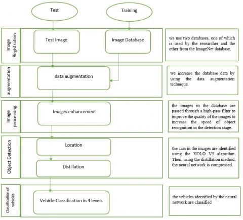
A combination of the MobileNet neural network with the YOLO V5 algorithm used in the proposed method is an acceptable solution that can increase the processing speed and overcome challenges such as weather conditions and a variety of vehicles. Figure 1 shows steps for the detection and classification of vehicles. In this method, using of multiple images taken from different angles of the vehicle increases the accuracy of object recognition. At the same time, speeding up the process of vehicle recognition on highways and checkpoints can also be counted among the capabilities of this system. The different steps used in this method are as follows: Image Registration, Image Processing, Object Detection and Vehicle Classification.
Figure 1. Steps for detection and classification of vehicles
3.1 Images registration
In the image registration section of the proposed method, images are prepared from different databases. We use two databases. The first one is ImageNet, and the second one is a database we created ourselves. The created database is made of images at different weather conditions. The database created is 7404 images, and these images are prepared from video frames in such a way that one frame is extracted from a video every second. The images resolution of each image is 512×512.
These images are divided into four classes: cars, SUVs, trucks, and buses.
Then, for annotation, using four colors, we teach the labeling of two database images on each pixel, 60% of these images are used for training and 40% for testing.
3.2 Image augmentation
Increasing the accuracy in various conditions requires a data augmentation method. Data augmentation helps obtain new images for training by artificially producing new images from the original images. The use of acceptable new images to increase the collection size is the goal of the data augmentation.
As a modern deep-learning algorithm, convolutional neural networks (CNN) are capable of learning location-independent features. Nonetheless, what helps more to learn independent features in the image is to enhance and add data by rotation, changing light and color. All cases eventually lead to the fact that if the object in the image is rotated in any direction, or we face a decrease in light and transparency, etc., the network learns well to recognize correctly.
The following is Table 1 with information from the database.
Table 1. Information about databases
|
Database Type |
Number of Vehicles Before Applying Data Augmentation |
The Number of Vehicles After Applying Data Augmentation |
Images in Adverse and Noisy Weather Conditions |
|
Database Created |
7404 |
73200 |
7200 |
|
Database ImageNet |
6300 |
45040 |
4700 |
|
Total |
13704 |
118240 |
11900 |
3.3 Image processing
Convolutional masks are used in the proposed method. When different convolution or spatial masks are applied to the same image, it produces different results. In the proposed method, a high-pass filter is used. These filters are those spatial filters that maintain or improve high-frequency components including fine details, points, lines, and edges with possible effects of increasing noisy pixels. In other words, it highlights the changes in brightness of the image. By using this filter in our method, the issue of separating objects has been solved. Applying the convolution mask on the images makes the image smaller and the network does not appear in the image in general. In the proposed method, because the Yolo algorithm is used when all the details of an image are clear and prominent, this algorithm can separate the components of an image from each other in the image, and the detection speed is also higher (reducing the calculation load).
3.4 Object detection
It is necessary to create an algorithm that can recognize objects by implementing itself in these networks. SSD, YOLO, small face, and small sample segmentation techniques, including R-CNN, and U-Net are several algorithms that are used to identify the type of vehicles. Among these, an algorithm like YOLO has been attractive due to its high power of object detection the completeness of the deep learning system, and the speed of solving the problem. The function of this algorithm is that it first separates and decomposes the image into different parts, and by marking each part and simultaneously running the detection algorithm, it categorizes the parts and draws the final result. After the object detection process is done completely, it connects them such that the two parts of each main object are a box. As all these actions are performed simultaneously and in parallel, it is possible to continuously process up to 40 images per second.
Here, version 5 of the Yolo algorithm is used. YOLO V5 is different from all previous versions. In YOLO V5, the backbone part (in the network architecture) is of CSP type and the neck part is of PA-NET type [20]. The major improvements of this version include mosaic data augmentation and automatic learning of bounding boxes. YOLO V5 is small. Specifically, the size of a weights file (with the extension) for YOLO V5 is 27MB. YOLO V5 is almost 90% smaller than other versions. It is very fast and light compared to other versions, while its accuracy is equal to the standard of other versions [20].
3.5 Vehicle classification
The proposed algorithm for labeling each vehicle in four levels (rider, SUV, truck, and van) must be implemented on a neural network. A convolution neural network is used to implement this operation. The commonly used convolutional neural networks for this purpose are Imagenet, Li-net, Alexnet, ZFnet, VGGnet, Googlenet, and Rosenet.
The need for small-sized and high-speed networks with the ability to be used in robotics, minicomputer boards, and of course mobile phones exists in all systems.
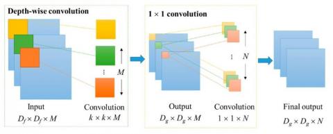
MobileNet neural network is one of the most prominent small-size networks. A new type of convolution called depth-wise separable convolution is introduced in the MobileNet neural network. The main element in the MobileNet network is this convolution layer. Depth-wise separable convolution is the heart of the MobileNet network. The standard convolution in Qaleb neural networks included two stages of filtering and integration. Depth-wise separable convolution also includes two stages of filtering and integration. However, each step has small differences from standard convolution steps. One difference is that in depth-wise convolution, there is separable in both stages of convolution. While in standard convolution, there is convolution only in the filter stage. The integration step is a simple addition. The two stages of depth-wise separable convolution are like this:
The first stage is filtering, and depth-wise convolution, and the second stage is integration and point-wise convolution.
3.5.1 Depth-wise convolution
Depth-wise convolution is equivalent to standard convolution filtering. But with an important difference. We had a k×k kernel in the standard M convolution. But in depth-wise separable convolution, we have a k×k kernel.
First, by performing the filtering operation, each page of the kernel is channelized into one page of the F input feature champ. This stage is called deep convolution. Because we have done convolution on each page in line with the depth or pages and did not add the output pages together.
3.5.2 Point-wise convolution
This step is equivalent to the integration step in standard convolution. But there is still a fundamental difference between the integration stage in standard convolution and depth-wise separable convolution. In the standard M convolution, we had k×k kernels. But in this convolution, we have only one k×k kernel.
MobileNet neural network has 4.2 million parameters. When we compare the number of parameters of this network with the popular ResNet-18 network with 11 million parameters, the amount of parameters is much less than the other neural network.
In the MobileNet neural network, 94.86% of the calculation volume is in the same 1×1 Convolution layer. The important thing is that with an interesting idea, most numbers of the calculations and the number of parameters have been reduced in 3×3 Convolution layers.
An overview of a depth-resolvable torsion block is shown in Figure 2.
Figure 2. Overview of a depth-wise separable convolution block
Considering the mentioned advantages and the important problem of reducing the calculation load (processing speed), we use this neural network.
3.6 Proposed neural network coefficients compression
We will see better performance when the number of parameters increases. Of course, this case leads to an increase in computing costs, which subsequently affects the cost imposed on the server and the increase in the duration of training. For this reason, cost improvement and management is achieved by compressing the neural networks that it is necessary.
• Weight pruning
One of the oldest methods in neural network compression is weight pruning, which refers to the removal of certain connections between neurons. This deletion in practice means that the deleted weight is replaced by zero.
• Quantization
The essence of a neural network is a combination of linear algebra and some other operations. By default, most systems use a variety of float32 formats to represent variables and weights.
However, the calculation speed with other formats such as int8 is generally higher than float32 formats and occupies less space in memory.
Neural network quantization refers to methods that take advantage of this. Changing the longer format to a shorter one (e,g, from float32 to int8).
• Distillation
Among the three neural network compression methods, the distillation method has been used because of its capabilities, which has more advantages than the two methods of pruning and quantization. Despite the effectiveness of quantization and pruning methods in implementation, their possible damages such as loss of weights and neurons of neural network may lead to a decrease in network accuracy.
The simple approach of the distillation method is training a large model (teacher) to achieve the best performance and using its forecast to teach a smaller network (student) which is easily implementable. With this method, deep neural network helps the smaller network to estimate the main function.
The calculation diagram of the distillation method is shown in Figure 3.
The diagram of the distillation method is shown in Figure 4.
Figure 3. Graph of distillation method calculations
Figure 4. Distillation method implementation diagram
The probabilities obtained from the hefty model, which are soft targets for the training of the small model, provide the generalization of transferring the heavy model to the smaller model. Therefore, this training kit or a "transfer kit" for hefty model training can be used in the transfer phase. Since simpler models are a subset of heavy models, we can use each of those simple models as soft targets by estimating arithmetic or geometric averages. Due to the high entropy of soft targets and the provision of more information for training and their less diversity compared to hard targets, it is possible to train a small model without the need for heavy model data and only with appropriate data while achieving an increase in the learning rate. Although the training time cannot be improved much in the distillation method, the conclusion time of the distilled models has been improved. This is one of the major differences between this method and the previous methods.
3.7 Implementing the proposed method
Using Python, the proposed method composed of (YOLO V5 algorithm and MobileNet neural network) is implemented. The proper design of this program has been very effective for quick sampling of complex programs. In the proposed method, the Keras library is used for implementation. This library is open source in Python and can be implemented on Tensor Flow, Microsoft Cognitive Toolkit, R Theano, or PlaidML.
Defining and training neural network models using a few lines of code during implementation is one of the capabilities of this library. Finally, the MobilNet neural network and the YOLO V5 algorithm can be installed by existing libraries.
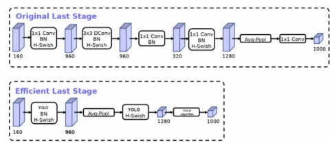
In the design of the neural network, the MobileNet neural network is first implemented, then to increase the processing speed (reduce the calculation load) and recognize the desired object, the YOLO algorithm is used in the convolution layers. This integration reduces parameters and operations, which increases both accuracy (due to the use of MobileNet neural network) and processing speed (YOLO algorithm).
The shape of the network redesign and new layering is shown in Figure 5.
To improve the performance of the designed network, the computationally expensive layers at the beginning and end of the network have been redesigned. To increase the speed of detection, the Yolo algorithm has been used instead of the convolutional layer.
A new non-linear function, h-swish, is used instead of the linear ReLU, which has a great effect on improving the performance of the network.
In addition to the initial layers, there are a number of final layers in this version that require a lot of computation and slow down the network even more. To reduce the amount of computation and to increase the speed of the network, the average pooling layer of the last block is moved and placed before the expansion layer of the last block. This greatly reduces the amount of computation by using the average pooling layer. Also, the depth and point convolution layers in the last block are unused and we remove them from the mesh. The resulting image is in Figure 5:
Figure 5. The shape of the network redesign
This redesign reduces the latency to 7 milliseconds or 11% of the execution time. On the other hand, these changes reduce the total number of additions and multiplications in the network by 30 million, without any loss of accuracy.
One of the non-linear functions whose use improves the accuracy of neural networks is the swish function, which is calculated by the following relationship:
$Swish \, x=x \cdot \delta(x)$ (1)
Instead of using the swish function, the h-swish function is used, which has almost the same behavior as the swish function and is calculated using the following relationship.
$h-Swish =x \frac{{Relu}(x+3)}{6}$ (2)
3.8 Converting the proposed neural network to Android application
Python does not have built-in development capabilities for the Android operating system, but some packages can be used to create Android applications. Different types of methods to convert Python to Android are:
(1) Kivy
This tool can be run on Android and to some extent on any device with OpenGL ES version 2 (and at least Android 2.2). Kiwi Android software is common and Android software that can be distributed on platforms like PlayStore and other software of this operating system.
(2) BeeWare
Android support in Beeware is possible through the use of VOC (a tool for compiling Python codes to Java files). This process enables Python code to run on the JVM just like Java code.
(3) Chaquopy
It is a plugin for Android Studio.
(4) Pyqtdeploy
It is a tool for loading PyQt programs and supports loading operations on PC (Linux, Windows, and OS X) and mobile platforms (iOS and Android).
(5) QPython
It is an installable scripting engine and a programming environment.
(6) SL4A
The Android Scripting Layer or SL4A, formerly called the ASE (Android Scripting Environment), is a set of "facades" that are a highly simplified subset of the API.
(7) PySide
It is a Python connector package for Qt that also supports Android at basic levels.
(8) Termux
Termux is an example of an Android terminal and a Linux environment that can be used directly without the need for installation and configuration.
According to the above definitions, we use the powerful Kivy framework to build an Android application. Kivy is a Python module that allows the creation of compatible programs using Python. It is very easy to reuse the same code on IOS, Android, Mac, Windows, Linux, and almost all other operating systems with this module.
The main advantage of Kivy are:
•It is based on Python, which is very powerful given the rich nature of the library.
•Use a fixed code on all devices
•Easy tools with multi-touch support.
•Better performance than cross-platform HTML5 alternatives.
The architecture is divided into two levels: high level and low level. The top level contains the tools and features available to GUI developers, such as widgets, the Kivy language, and other high-level features visible to the developer. In contrast, the low level contains the tools that make up the Kivy infrastructure.
High Level: This section contains the tools and features available to GUI developers, such as widgets, the Kv language, and other high-level features visible to the programmer.
Low Level: In contrast, this section contains tools that show what the Kivy infrastructure is and what it contains.
The architecture of the Kivy framework is as follows.
"Input Provider" and "Core Provider": First, we want to know what the concept of "abstraction" is in the Kivy architecture. Therefore, we need to know that it is one of the main concepts of the Kivy framework and it means to hide technical details and present a view is simpler than that. The concept of abstraction allows developers to work with high-level features without having to understand the low-level details of the system. In the "core provider" section, the Kivy framework abstractly provides basic tasks such as opening a window, displaying images and text, playing audio, receiving images from the camera, spell spell-checking. This allows programmers to develop their applications quickly and easily without having to understand the technical details and inner workings of these tasks. Operating systems use different software programming interfaces to perform basic tasks.
A kernel provider is a piece of code that uses APIs specific to operating systems such as MacOS, Linux, BSD, Unix and Windows to act as an intermediate communication layer between the Kivy framework and the operating system. This module is responsible for performing key system-related tasks based on the operating system's specific API and for passing information between Kivy and the operating system. In a similar concept, "Input Providers" are pieces of code that support a specific input device, such as Apple trackpad and mouse emulator, and if you need to add support for a new input device, you can simply create a new class that reads the data from the target device and converts it into "Basic Events" of this framework.
"Graphics API" of the Kivy framework is an abstraction of OpenGL. In other words, this framework has provided a level of abstraction that allows programmers to create various geometric shapes without directly using complex OpenGL code, using the tools and facilities provided in Kivy. One of the advantages of using this graphical interface is the ability to automatically optimize drawing commands, helping to improve the performance of programs.
The core: The core of the Kivy framework provides the following features:
Clock: This feature is used to schedule timer events. In other words, developers can easily manage time-based operations and decide which parts to run periodically and which parts to run once and at a specific time.
Cache: If data is used frequently, it is easy to use the Cache class provided in the Kivy framework for time-management purposes-without the programmer having to write a lot of code for this purpose.
Gesture recognition: The gesture recognition module analyses the user's movements on the input device to detect certain patterns. These patterns-such as circles and rectangles-can be used to control a device or perform a specific action.
Kivy language: The Kivy design language is designed to describe graphical interfaces easily and efficiently.
Properties: Properties in Kivy are classes used to communicate between widget code and the structure of GUI elements defined by the developer, and are different from the usual Python properties.
UIX: The UIX module provides a set of widgets and layouts to quickly and easily create user interfaces within this framework.
Modules: Module classes in Kivy add new functionality to applications, like plug-ins in web browsers.
Input events: In the Kivy framework, different types of input sources such as touch, mouse, TUIO, etc. are managed using the abstraction concept. Input events in this framework are defined by instances of the Touch class, which are in one of three states: "up", "down" and "in motion".
Widgets and event dispatching: In the previous parts we learned what a widget is in Kivy. We should mention again that widgets are the basic elements to describe the part of the application that receives "input events" from the user. For example, when the user taps a button, the button widget detects that a touch event has occurred and triggers the appropriate response. It is a fact that widgets have a tree structure and a widget can have zero or a number of children. Therefore, in the widget tree there is only one main widget or "root" for which no parent is defined, and other widgets are directly or indirectly children of this root. When a new event occurs, for example "touch", an event is sent for each touch, which is first received by the main widget or root of the widget tree. Then, depending on the type of widget, this event is directed to the appropriate widget-we call this operation "event dispatching"-to respond correctly to the desired event. In general, the widget tree represents the hierarchical structure of these graphical elements, and the input events are correctly distributed and processed by this tree.
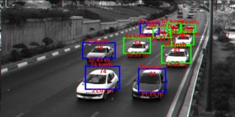
3.9 Speed tracking
In order to detect the speed of the vehicle, the speed can be obtained by calculating the displacement of the pixels in the frames.
How to track the speed is shown in Figure 6.
Figure 6. How to track speed
IDLE software is used to implement the proposed method. All execution steps are performed on a Window10 operating system, Intel Core i7 processor, 12GB DDR3 memory running at 799.5 MHz16 and NVIDIA GeForce GTX 750 Ti graphics card.
To prove the efficiency of this device, 130,000 car images have been used. These images are from films made by the researcher in different weather conditions, including mountainous, desert and rainy. In the previous methods, problems such as geographic conditions were not given importance, which caused challenges such as decreasing accuracy in atmospheric conditions, mountains and intense light radiation in desert areas.
Apart from the database that is prepared, the ImageNet database is also used. A data augmentation technique has been used to increase the accuracy and better train the neural network.
To check the performance, the proposed method is performed with two RFCN neural network methods and the combination of YOLO algorithm with VGG neural network.
In the proposed method, despite the continuous working hours of the device, less than 2% losses were obtained, while in the RFCNN method, this loss coefficient is almost 9%. The corresponding function displays the error coefficient during the execution of the neural network and in the combination of YOLO algorithm with VGG neural network method, this loss coefficient is almost 2.5%. As follows:
Loss $=\frac{1}{\mathrm{~N}} \sum_{\mathrm{i}=1}^{\mathrm{N}}\left(\mathrm{y}_{\mathrm{P}}-\mathrm{y}_{\mathrm{t}}\right)^2$ (3)
In addition to the continuous and adequate performance in this device, the error rate of non-diagnosis of the device in this method has been reduced and the effectiveness has been close to 98%. What increases the accuracy of detection to almost 98% in the implementation of this method is the use of MobileNet convolution with the YOLO V5 algorithm and the use of a spatial filter with high processing speed. While the RFCNN method has an efficiency of 91%. In another implementation we use the YOLO algorithm with the VGG neural network method has an efficiency of 97%.
Accuracy $=\frac{\mathrm{T}_{\mathrm{R}}}{\mathrm{T}_{\mathrm{R}}}$ (4)
The Precision is the percentage of the correct detection of the vehicle compared to the total number of vehicles and is calculated through formula (3).
In our method, about 98 out of 100 images are correctly recognized, and the precision is roughly 98%, while in the RF-CN neural network method, about 90 out of 100 images are correctly recognized, abd thus the precision is about 90%. In another implementation we use the combination of YOLO algorithm with VGG neural network about 96images out of 100 images are correctly recognised.
Precision $=\frac{\mathrm{T}_{\mathrm{R}}}{\mathrm{T}_{\mathrm{R}}}+F_R$ (5)
In our proposed method, by using several techniques (spatial filters, data augmentation), the execution time has been reduced to approximately 0.1 seconds, while in the RFCN neural network method, the execution time is approximately 0.25 seconds. In the proposed method, the learning rate is divided by 10 once every 50 rounds becoming smaller over time. The learning rate is often represented by the symbol α and sometimes by the symbol η and represents the weights updating speed, which can be a fixed value or changes to an adaptive one. In this method, learning is performed in batches, that is, instead of all the training data being applied to the network at once, they are entered into the neural network in batches and in turn. In the proposed method, the processing speed of vehicle detection has been improved, and the reason for that is the use of the Yolo algorithm. This algorithm is executed in parallel for all sections to see which category each section belongs to. After the complete identification of objects, it connects them together and detects the type of vehicle. This algorithm is real-time and is able to identify 40 objects in one image and solves the problem of multiple images. At the same time, this algorithm has reduced the learning rate in the training process, the training time, and improved the processing speed, which, as a result, reduces the calculation load and increases the object recognition accuracy compared to the RFCN method.
In addition, compared to the method of combining YOLO algorithm with VGG neural network, although both algorithms are similar, in the proposed method, since the presented neural network has a smaller volume, the computational load is reduced.
Mean Squared Error (MSE)-MSE is a network performance function. It measures the network's performance according to the mean of squared errors. The mean squared error is the squared error averaged over the M*N array.
$\operatorname{MSE}=\frac{1}{M N} \sum_{i=1}^{i=M} \sum_{j=1}^{j=N}\left(F_1(i . j)-F_2(i . j)\right)^2$ (6)
The neural network's validation RMSE (root mean square error) recorded every 104 backpropagation iterations during its training.
RMSE $=\sqrt{M S E}$ (7)
Peak signal-to-noise ratio (PSNR)-The PSNR is an expression for the ratio between the maximum possible power level of a signal and the power of distorting noise that affects the quality of its representation.
$\mathrm{PSNR}=10 \text {Log} \left(\frac{255^2}{\mathrm{MSE}}\right)$ (8)
Coefficient of Correlation (COC)-gives the correlation coefficient between the simulated values and the actual values. The value of the correlation coefficient varies between zero and one. The value of the correlation coefficient is 0 where there is no correspondence between the values. The correlation coefficient will rise as the relationship between the simulated values and the implemented values increases. A perfect match will have a factor of one. COC is calculated using Eq. (9):
$\begin{aligned} & \text { Correlation(r) } =\frac{\mathrm{N} \sum \mathrm{XY}-\left(\sum \mathrm{X}\right)\left(\sum \mathrm{Y}\right)}{\operatorname{sqrt}\left(\left[\mathrm{N} \sum \mathrm{X} 2-\left(\sum \mathrm{X}\right) 2\right]\left[\mathrm{N} \sum \mathrm{Y} 2-\left(\sum \mathrm{Y}\right) 2\right]\right)}\end{aligned}$ (9)
where,
N= number of pixels of the image,
X= input image, Y= output.
The results of PSNR, RMSE and COC calculations for the proposed method and the RFCN method are shown in Table 2.
One of the advantages of this system is its correct performance in different weather conditions and geographical positions, so 11,900 images of passing cars on different roads and in different weather conditions were tested around the clock to check the performance of this system.
The calculation results of the proposed method, the RFCN method and the combination of the YOLO algorithm with the VGG neural network method are given in Tables 2-8.
Table 2. Calculation results
|
Methods |
PSNR |
RMSE |
COC |
|
Propose method |
40.0135 |
8.7362 |
0.0729 |
|
RFCN method |
34.4664 |
23.4339 |
-0.0521 |
|
the combination of YOLO algorithm with VGG neural network |
38.0135 |
10.3545 |
0.0956 |
Table 3. Calculation results of the proposed method
|
Vehicle Type |
Loss |
Accuracy |
Rate Learning |
|
Riding |
0.214 |
98.73% |
0.0010 |
|
Truck |
0.278 |
98.47% |
0.0010 |
|
Long Undercarriage |
0.268 |
98.55% |
0.0010 |
|
Bus |
0.254 |
98.63% |
0.0010 |
Table 4. Calculation results of the RFCN method
|
Vehicle Type |
Loss |
Accuracy |
Rate Learning |
|
Riding |
0.7736 |
87.48% |
0.02 |
|
Truck |
0.7841 |
86.79% |
0.02 |
|
Long Undercarriage |
0.7753 |
88.13% |
0.02 |
|
Bus |
0.7743 |
%87.48 |
0.02 |
Table 5. Calculation results of the combination of YOLO algorithm with VGG neural network method
|
Vehicle Type |
Loss |
Accuracy |
Rate Learning |
|
Riding |
0.3749 |
97.97% |
0.010 |
|
Truck |
0.3641 |
97.22% |
0.010 |
|
Long Undercarriage |
0.3689 |
97.55% |
0.010 |
|
Bus |
0.3678 |
96.63% |
0.010 |
Table 6. Calculation results of the proposed method
|
Epoch |
Iteration |
Time Elapsed(s) |
RMSE |
|
1 |
1 |
4 |
0.017 |
|
1 |
200 |
1.3 |
|
|
2 |
400 |
2.56 |
|
|
3 |
600 |
4.20 |
|
|
3 |
800 |
5.30 |
|
|
4 |
1000 |
7.07 |
0.11 |
|
5 |
1200 |
8.30 |
0.12 |
|
5 |
1400 |
9.50 |
|
|
6 |
1600 |
11.10 |
0.13 |
|
7 |
1800 |
12.30 |
0.17 |
|
7 |
2000 |
13.50 |
|
|
7 |
2065 |
14.15 |
Table 7. Calculation resultsof the RFCN method
|
Epoch |
Iteration |
Time Elapsed(s) |
RMSE |
|
1 |
1 |
3 |
0.088 |
|
1 |
200 |
1.32 |
|
|
2 |
400 |
2.48 |
|
|
3 |
600 |
4.27 |
|
|
3 |
800 |
5.47 |
|
|
4 |
1000 |
7.33 |
0.25 |
|
5 |
1200 |
8.23 |
0.22 |
|
5 |
9.53 |
1400 |
|
|
6 |
1600 |
11.16 |
0.27 |
|
7 |
1800 |
12.37 |
0.26 |
|
7 |
2000 |
13.51 |
|
|
7 |
2065 |
14.17 |
Table 8. Calculation resultsof the combination of YOLO algorithm with VGG neural network method
|
Epoch |
Iteration |
Time Elapsed(s) |
RMSE |
|
1 |
1 |
3.5 |
0.028 |
|
1 |
200 |
1.31 |
|
|
2 |
400 |
2.47 |
|
|
3 |
600 |
4.26 |
|
|
3 |
800 |
5.45 |
|
|
4 |
1000 |
7.31 |
0.19 |
|
5 |
1200 |
8.21 |
0.18 |
|
5 |
1400 |
9.51 |
|
|
6 |
1600 |
11.14 |
0.21 |
|
7 |
1800 |
12.34 |
0.21 |
|
7 |
2000 |
13.51 |
|
|
7 |
2065 |
14.17 |
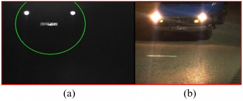
The proposed method can correctly recognize 98 out of 100 images, and in the RFCN method this number is 91, and in the combination of YOLO algorithm with VGG neural network this number is 96. Another important point is the execution time of this proposed method due to the use of the distillation technique and the YOLO V5 algorithm and the Mobilenet neural network, which, as mentioned above, is around 0.1 seconds, which is significantly different from 0.25 seconds in other methods. As you can see in the Figure 7, image 7(a) was recorded by the camera when the car passed, and Figure 7(b) is the reconstructed image under the same conditions, with the improvement of the image quality by the detection device.
This method has been implemented using 7737 images recorded at night and 3614 images of separated frames from videos based on database images. Achieving image recognition accuracy with a factor of 96% in conditions where the images are separated from the video or recorded at night shows the proper performance of this method. While accuracy in the RFCN method in the same conditions is almost 81%. Of course, some mistakes of the neural network in the diagnosis due to the similarity of the types of cars are also undeniable. but in the combination of YOLO algorithm with VGG neural network accuracy in the same conditions is almost 89%.
The impossibility of recording the image of all the components of the vehicle is one of the reasons for not correctly identifying the vehicle. Taking a picture of a part of the car cannot help in this case, and it requires extensive imaging to separate the vehicles from each other and identify them better. With this method, the level of sensitivity is reduced to see the image better and separate vehicles from each other more accurately.
Vehicles in bad weather conditions (snow), adverse weather conditions, implementation device, separation of vehicles are given in Figures 7-11.
Figure 7. Vehicles in low light conditions
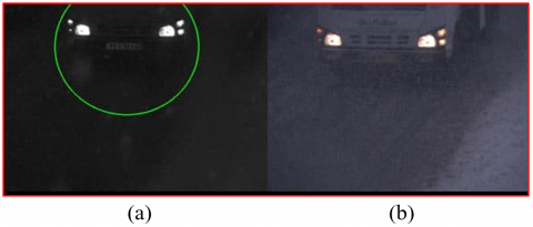
Figure 8. Vehicles in bad weather conditions (snow)
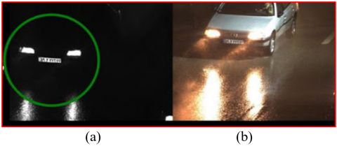
Figure 9. Adverse weather conditions
Figure 10. Implementation device
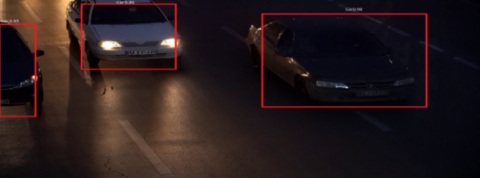
Figure 11. Separation of vehicles
Based on statistical analysis, we compare the proposed method with the vehicle network detection method using the R-FCN neural network and combining the YOLO algorithm with the VGG neural network, which has the following innovations compared to these methods.
a) Vehicle detection accuracy:
The results show that in different environmental conditions and the simultaneous presence of several types of vehicles in the image, the proposed method can perform a more accurate classification than the R-FCN method. The total efficiency of four classes in the proposed method is about 98% and in the R-FCN method, it is about 91% and the combination of the YOLO algorithm with the VGG neural network method has an efficiency of 97%.
Since the MobileNet convolution neural network and YOLO algorithm along with spatial filter are used, the processing speed of calculations is increased and as a result, the performance of accuracy has increased compared to those of the other methods (object detection) compared to the R-FCN method. In the proposed method, due to the use of a spatial filter, the objects in the frame of an image are more prominent, which causes a better recognition of the object in the image in the before-processing part, further, the use of the MobileNet neural network along with the Yolo algorithm has a significant effect on increasing the accuracy of vehicle detection.
b) Processing speed:
In the proposed method, the processing speed is approximately 0.001 seconds, and in the R-FCN method, it is 0.02 seconds, and the combination of the YOLO algorithm with the VGG neural network, it is 0.01 seconds.
In the proposed method, the processing speed of vehicle detection has been improved, and the reason for that is the use of the Yolo algorithm. This algorithm is applied to all sections in parallel, regardless of which category each section falls into. After the complete identification of the objects, it connects them, and detects the type of vehicle. This algorithm is real-time and can identify 40 objects in one image and solves the problem of multiple images. This algorithm has reduced the learning rate in the training process, and the training time and improved the processing speed.
Another reason the proposed method improves the performance of the processing speed and that is the use of a spatial filter. By highlighting the objects of an image, the spatial filter improves the performance of the processing speed in the proposed method.
c) Accuracy criteria:
In the proposed method of the YOLO algorithm, it has correctly recognized about 98 images out of every 100 images the accuracy is about 98%. Therefore, the detection of the desired object in the proposed method has increased compared to the R-FCN method and the YOLO algorithm with the VGG neural network.
The reason for the high accuracy standard in the proposed method is the use of the image registration method before pre-processing. First, in image registration, images are collected and prepared from different databases. It is worth mentioning that the researcher has also collected pictures of different environmental conditions in the country. First, noise removal is done before preprocessing, and it is done with image quality improvement processes. The process of improving image quality results in more suitable images for display or image processing.
d) Detection accuracy in different atmospheric conditions and noisy images:
In our method, in the image registration section, images are first collected and prepared from different databases. It is worth mentioning that the researcher has also collected images from different environmental conditions of the country, these images were prepared from different weather conditions of the country. Then, using spatial filter and data augmentation techniques, the image is prepared for processing. This has increased the accuracy in different atmospheric conditions and noisy images, and the vehicle detection accuracy is about 96%.
e) Multiplicity of images:
The proposed method, using the Yolo algorithm, will be able to identify 40 objects in the image at the same time.
f) Separation of vehicles that overlap each other:
Depending on the selection of different weights, a wide range of image processing operations can be performed through convolution.
The utilization of the Yolo algorithm has made it possible to separate the components of an image from each other when all details are clear.
Practical applications of the proposed method
The ability to charge intelligent tolls
Thanks to the registration of all traffic, the system can be used to collect tolls.
In addition, if it is necessary to apply restrictions and obstacles based on the type of vehicles or their number plates, this can easily be done, for example.
- Prohibiting heavy vehicles during the day.
- Prohibiting heavy vehicles from using a particular road on public holidays.
- Scope of the traffic plan.
- Prohibiting public vehicles on suburban roads.
- Traffic of government vehicles in the desired area.
- Traffic of special vehicles (ambulances, disabled vehicles, buses, etc.) on emergency lanes.
Limitations of the proposed method
Considering that the efficiency is around 98%, but there are still limitations such as blurred images, we need a more powerful processor.
It is suggested that due to limitations such as the processing speed of objects in the images, the trained neural network in the proposed method was compressed, resulting in the loss of a small amount of trained data, thus requiring hardware with high processing power, such as FPGA implementation. In FPGA, there is no need to compress the network as it has powerful processors for data processing.
It can be concluded that the combined method of the YOLO V5 algorithm and the Mobilenet neural network has an acceptable performance in detecting the type and speed of vehicles, and the possibility of implementing and exploiting it as an Android application is one of the other features of this method. Also, based on the results obtained, the implementation of this method shows its better performance compared to other methods. In this method, features such as: increasing the accuracy of vehicle detection, reducing the calculation load, increasing the accuracy criterion, detection accuracy in different atmospheric conditions, solving the problem of multiple images, separating vehicles that have overlaps, using different databases for better training as well as size reduction of the neural network.
[1] Stewart, B.D., Reading, I., Thomson, M.S., Binnie, T.D., Dickinson, K.W., Wan, C.L. (1994). Adaptive lane finding in road traffic image analysis. In Seventh International Conference on Road Traffic Monitoring and Control, 1994. London, UK, pp. 133-136. https://doi.org/10.1049/cp:19940441
[2] Zhigang, Z., Huan, L., Pengcheng, D., Guangbing, Z., Nan, W., Wei-Kun, Z. (2018). Vehicle target detection based on R-FCN. In 2018 Chinese Control And Decision Conference (CCDC), Shenyang, China, pp. 5739-5743. https://doi.org/10.1109/CCDC.2018.8408133
[3] Hadi, R.A., Sulong, G., George, L.E. (2014). Vehicle detection and tracking techniques: A concise review. arXiv Preprint arXiv: 1410.5894. https://doi.org/10.5121/sipij.2013.5101
[4] Kim, J.B., Park, H.S., Park, M.H., Kim, H.J. (2001). A real-time region-based motion segmentation using adaptive thresholding and K-means clustering. In AI 2001: Advances in Artificial Intelligence: 14th Australian Joint Conference on Artificial Intelligence Adelaide, Australia, Springer Berlin Heidelberg, 14: 213-224. https://doi.org/10.1007/3-540-45656-2_19
[5] Enkelmann, W. (1991). Obstacle detection by evaluation of optical flow fields from image sequences. Image and Vision Computing, 9(3): 160-168. https://doi.org/10.1016/0262-8856(91)90010-M
[6] Won, Y., Nam, J., Lee, B.H. (2000). Image pattern recognition in natural environment using morphological feature extraction. In Advances in Pattern Recognition: Joint IAPR International Workshops SSPR 2000 and SPR 2000 Alicante, Spain, Springer Berlin Heidelberg, pp. 806-815. https://doi.org/10.1007/3-540-44522-6_83
[7] Nasehi, M., Ashourian, M., Moalem, P. (2020). An overview of the type of vehicle detection techniques. Majlesi Journal of Telecommunication Devices, 9(3): 133-137. https://doi.org/10.30486/mjtd.2023.1990441.1040
[8] Li, J., Liu, Y., Tageldin, A., Zaki, M.H., Mori, G., Sayed, T. (2015). Automated region-based vehicle conflict detection using computer vision techniques. Transportation Research Record, 2528(1): 49-59. https://doi.org/10.3141/2528-06
[9] Tang, T., Zhou, S., Deng, Z., Zou, H., Lei, L. (2017). Vehicle detection in aerial images based on region convolutional neural networks and hard negative example mining. Sensors, 17(2): 336. https://doi.org/10.3390/s17020336
[10] Dubuisson, M.P., Jain, A.K. (1995). Contour extraction of moving objects in complex outdoor scenes. International Journal of Computer Vision, 14(1): 83-105. https://doi.org/10.1007/BF01421490
[11] Oliveira, M., Santos, V. (2008). Automatic detection of cars in real roads using haar-like features. Department of Mechanical Engineering, University of Aveiro, 3810. https://www.researchgate.net/publication/267863282_Automatic_Detection_of_Cars_in_Real_Roads_using_Haar-like_Features.
[12] Huang, R., Pedoeem, J., Chen, C. (2018). YOLO-LITE: A real-time object detection algorithm optimized for non-GPU computers. In 2018 IEEE International Conference on Big Data (Big Data), Seattle, WA, USA, pp. 2503-2510. https://doi.org/10.1109/BigData.2018.8621865
[13] Li, Y., Song, B., Kang, X., Du, X., Guizani, M. (2018). Vehicle-type detection based on compressed sensing and deep learning in vehicular networks. Sensors, 18(12): 4500. https://doi.org/10.3390/s18124500
[14] Hicham, B., Ahmed, A., Mohammed, M. (2018). Vehicle type classification using convolutional neural network. In 2018 IEEE 5th International Congress on Information Science and Technology (CiSt), Marrakech, Morocco, pp. 313-316. https://doi.org/10.1109/CIST.2018.8596500
[15] Sheng, M., Liu, C., Zhang, Q., Lou, L., Zheng, Y. (2018). Vehicle detection and classification using convolutional neural networks. In 2018 IEEE 7th Data Driven Control and Learning Systems Conference (DDCLS), Enshi, China, pp. 581-587. https://doi.org/10.1109/DDCLS.2018.8516099
[16] Wang, X., Zhang, W., Wu, X., Xiao, L., Qian, Y., Fang, Z. (2019). Real-time vehicle type classification with deep convolutional neural networks. Journal of Real-Time Image Processing, 16: 5-14. https://doi.org/10.1007/s11554-017-0712-5
[17] Nasehi, M., Ashourian, M., Emami, H. (2022). Fast detection of vehicle type and position in images based on deep neural network. Scientific Journal of Electronical & Cyber Defence, 10(2).
[18] Nasehi, M., Ashourian, M., Emami, H. (2022). Vehicle type, color and speed detection implementation by integrating VGG neural network and YOLO algorithm utilizing raspberry Pi hardware. Journal of AI and Data Mining, 10(4): 579-588. https://doi.org/10.22044/jadm.2022.11915.2338
[19] Hicham, B., Ahmed, A., Mohammed, M. (2018). Vehicle type classification using convolutional neural network. In 2018 IEEE 5th International Congress on Information Science and Technology (CiSt), Marrakech, Morocco, pp. 313-316. https://doi.org/10.1109/CIST.2018.8596500
[20] Nelson, J., Solawetz, J. (2020). Responding to the Controversy about YOLOv5. Roboflow: Roboflow News.