Ying Tian![]() | Majid Khan Majahar Ali*
| Majid Khan Majahar Ali*![]() | Lili Wu
| Lili Wu![]() | Tao Li
| Tao Li![]()
© 2024 The authors. This article is published by IIETA and is licensed under the CC BY 4.0 license (http://creativecommons.org/licenses/by/4.0/).
OPEN ACCESS
The purpose of this research is to investigate the use of information visualisation in deep learning and big data analytics. First, we present a notion that is crucial to the production of visualisations: visualisation repositioning. We can relocate visualisations and extract data from static photos using a pattern recognition-based approach, which frees up more time for artists to create and lessens the workload of designers. Next, we present VisCode, an application that may be used to encode unprocessed data into static images for superior visualisation repositioning. VisCode offers two sorts of repositioning: thematic (which applies several colour themes for the user to select) and representational (which encodes raw data and visualisation types into static visualisation graphics in JSON format). In order to demonstrate VisCode's potential utility and usefulness in the information visualisation space, we conclude with a sample application that involves moving a colour density map visualisation.
information visualization, big data, deep learning, pattern recognition, VisCode
The rapid increase in data volume and the explosion of information have become commonplace in the current digital era. Technological advancements provide us access to vast amounts of data from multiple sources, many of which exhibit high-dimensional characteristics such as image data [1]. However, visualizing and understanding high-dimensional data is challenging. It is often difficult to reveal the inherent structure and qualities of such data using traditional 2D and 3D visualization techniques [2]. Therefore, developing visualization methods for high-dimensional data has become crucial. Over the past decade, two-dimensional (2D) visualization techniques have been the primary method for effectively representing data [3]. While these techniques have proven useful in various cases, researchers and analysts continue to seek new ways to overcome the limitations associated with two-dimensional visualization, such as redundancy in data point interpretation, ambiguous patterns, and limited representation range [4].
When dealing with high-dimensional data, machine learning techniques are essential. These techniques allow us to create lower-dimensional representations that can visualize potential correlations between data, thus enhancing our understanding of the data [5]. Humans are naturally adapted to a three-dimensional environment, where daily movements, interactions, and experiences are intuitive. Therefore, it is questionable why we should limit our understanding of the complexity of high-dimensional data within the constraints of a 2D paradigm. The current technological constraints force us to adapt to a 2D perspective [6].
By utilising the ability of human vision to detect patterns, trends, and anomalies, data visualisation seeks to facilitate the understanding of data meaning [7]. To aid comprehend, recall, and judge circumstances, sensory reasoning can simply be used in place of cognitive reasoning using well-structured visual representations. People of all skill levels can benefit from visual representations of data that increase its accessibility and interest in order to investigate and evaluate the phenomena it expresses [8]. The primary goal of data visualisation is to effectively communicate the meaning of data through the use of visually appealing representations that are appropriate for the data's properties.
A primary objective of data visualisation is to enhance individuals' consciousness and understanding of data [9]. When it comes to sharing visualisation information over the Internet, images are a more practical and extensively processed medium than sending massive amounts of raw data directly. However, once the original detailed information (such as data points, axes text, and colours) is converted into pixel values, it becomes challenging to reconstruct the original information from the created images [10]. We attempt to minimally disrupt the carrier visual design in order to encode additional information in order to tackle this challenge.
In this research, VisCode is presented, a framework that utilizes encoder-decoder networks to embed and extract hidden information in visualized images. The challenges related to the visualization of high-dimensional, large-scale data are explored, alongside various approaches to its visualization. A two-dimensional space with a few key variables can be used to represent high-dimensional data. Projection tracing can be utilized to identify intriguing low-dimensional perspectives, or more variables can be visualized in graphs with different aesthetic qualities. Techniques such as dithering and alpha blending are discussed for resolving the overlapping point problem in large-scale data. The visualization of interactive Web applications using R tools such as tabplot, scagnostics, and other packages is also covered.
The paper concludes by summarizing the key points of the work and discussing the likely future direction of machine learning-based approaches to high-dimensional data visualization. It is hoped that this paper will provide readers with a deeper understanding of the concepts and applications of high-dimensional data visualization techniques, enabling more creative and adaptable applications to real-world problems.
The field of data visualisation research is still expanding. Researchers are using developing technology and cognitive theories to better understand data as the world gets bigger. We are dedicated to figuring out how to accomplish this, particularly in light of the intricacy of high-dimensional and time-series data.
The concept of high-dimensional space is hard for humans to grasp. Diverse visualisation techniques have surfaced in recent years to tackle this issue. Dimensionality reduction is a key method in the study and visualisation of high-dimensional datasets. Modern nonlinear techniques like t-SNE and Umap are a step away from the original linear algorithms like Principal Component Analysis (PCA) and Multi-Dimensional Scaling (MDS) [11-15]. Finding the ideal dimensionality reduction settings is a challenging task, though. Incorrect distance computations, deceptive shapes, or exaggerated results can come from selecting the wrong parameters. Furthermore, dimensionality reduction may result in information loss and the inability to preserve all of the original dataset's properties [16-18].
Therefore, a variety of visualisation strategies are needed for analysing high-dimensional datasets. Unitary (also known as atomic) visualisation techniques are frequently used in this context; they employ distinct visual markers to represent each data item [19]. Aggregate visualisation methods, on the other hand, merge several data elements into a single visualisation aggregate. The capacity to display both general trends and specific anomalies is a benefit of unit visualisation [20]. Units also allow you to work directly with each data item, for example, by utilising tooltips to get more specific information. Kiviat charts, scatter plot matrices, pixel bar charts, and parallel coordinates are common techniques for unit visualisation.
Glyphs are now being utilised in DR graphs to highlight significant dataset dimensions. Our objective is to give data scientists and domain specialists an easily accessible integrated picture of the data. We chose to add glyphs to the DR plot in order to improve it for this reason. Each data record is represented as a glyph in a glyph-based visualisation, which is a tiny, independent visualisation object. The graphical characteristics of the glyph, such as size, shape, colour, and orientation, can be mapped to the dimensions of the data [21]. Subsets of dimensions can produce easily recognisable composite visual elements, and patterns combining more than three dimensions are easier to discern than other techniques.
Improving people's comprehension and perception of data is the main objective of data visualisation. Images are a more common and convenient way to share visualisation information than directly transmitting vast volumes of raw data [22]. It gets more challenging to extract the original data from the created images, such as data points, coordinate axis text, and colours, once the raw data has been converted into pixel values. By reducing interference, we try to incorporate more information into the visualisation design in order to overcome this difficulty [23].
Our suggested VisCode technology embeds and recovers hidden information from visual images using an encoder-decoder network. Figure 1 shows the three primary components that make up the VisCode model's structure:
Figure 1. Key components of the VisCode system
In Figure 1, in order to make it easier to identify prominent elements for visualisation, the visual significance network (b) first analyses the input graphical chart (a) and creates a visual importance map. Subsequently, the encoder network (c) incorporates encrypted data into the graphical diagram (a). The carrier graph image and the QR code image are incorporated into vectors through the feature extraction technique. These two vectors are then supplied into the automatic encoding stage after being joined (shown in the illustration as yellow rectangles). The user (e) receives the encoded image (d), which they can then digitally transmit to other people. If the user wants to view certain data that is concealed within the chart, they can upload the encoded image to the decoder network (f). The user obtains the decoded information (g) following data recovery and error correction.
The preparation phase, which consists of a text transformation model and a visual importance network, involves the visual importance network. We use a network to describe the visual importance of the input data graph since the semantic properties of data visualisation differ from those of natural images. The encoder network will be constrained by the importance maps that are produced. We transform the pure information into a series of QR codes rather than binary data in order to address the error correction issue.
4.1 Aesthetic qualities or visual performance attributes
The constraint of visualising data is that it can only be represented in two dimensions. In statistics, a scatterplot is typically used to visualise two variables of continuous data; for three or more continuous variables, a scatterplot matrix may be utilised. More variables can be analysed together than with a scatterplot when using a scatterplot matrix, which is a scatterplot that pairs two variables and shows them as a matrix [24]. But as the number of variables rises, so does the size of the scatterplot matrix and the number of scatterplots that need to be looked at, which makes the whole more difficult to comprehend. Data visualisation gets more challenging as data complexity rises. Numerous approaches have been put out to solve this issue. First of all, it's a technique for including multiple variables into a single scatterplot by utilising visually striking characteristics like colour, size, and shape. Four variables are represented in a single scatterplot, for instance, if two continuous variables are shown in a scatterplot with one categorical variable displayed in a different colour for each category and another categorical variable displayed in a different shape for each category.
This scatterplot was used to conduct a high-dimensional, large-scale data visualisation study on the gender of the personnel, as seen in Figure 2. The size of the dots on the graph, as well as their colour, provide information about the number of individuals in the group (size). This allows for the expression of more information when all five variables are shown simultaneously in a single scatter plot. However, there is a feature that makes the information that the picture can convey evident, even though it expresses a lot of information in a single picture and is drawn in a sophisticated way.
To make the information easier to interpret, Figure 3 uses facets to divide the identical data as Figure 2 into four scatter plots. Rather than graphing all the data on one graph, the multifarious technique divides the data into categories of categorical variables. The multidimensional approach, in contrast to Figure 2, is helpful when there is a lot of overlap between data sets.
The ggplot2 package, which comes with R, is used in Figure 2 and Figure 3. Graph grammars [25], the theory of which was established by Wilkinson in 2006, are transformed by ggplot2 into a hierarchical syntax for graphs that is readily used in R. This one will assist you. A graph grammar is a collection of succinct definitions of graph elements organised as a grammar that covers everything from data to graph plotting. It includes statistical computation, which is broken down into seven phases: statistical, geometric, coordinate, and aesthetic. Variable selection, data transformation, algebra, scaling, and standard adjustment are all included in the grammar. This makes it easier to communicate information gleaned from the graph's data or conclusions.
Figure 2. Scatterplots of different shapes, colors and sizes
Figure 3. Scatterplot
Group A's 1,000 random numbers from uniform (0,1) and Group B's (800 random numbers from uniform (0,1) and 200 random numbers from N (0.7, 0.052) plots are shown in Figure 4.
Figure 4. Comparison of distribution maps
Data overlap is the main issue when it comes to visualising vast volumes of data. Group A and Group B's distributions are shown in Figure 4. Group B is made up of 800 random numbers created from a normal distribution with a uniform distribution between 0 and 1, a mean of 0.7, and a standard deviation of 0.05. Group A is made up of 1000 random numbers generated from a uniform distribution between 0 and 1. Group B's distribution is a random number with a 0.05 standard deviation and a mean of 0.7. There are 200 arbitrary numbers in it. Since most of the dots in the parallel dot plot (Figure 4 (a)) overlap, it cannot be properly referred to as a dot plot because it depicts 1000 dots between 0 and 1, one for each observation in each group. The display of this data does not show the difference in distribution between A and B as a line between 0 and 1. Figure 4 (b) depicts a box-and-line plot that is parallel to each group. The plot indicates that groups A and B have distinct median and quartiles, but the minimum and maximum values are the same. Though it is simple to use boxplots to evaluate the overall distribution, there are limits when attempting to obtain a thorough picture of the distributional properties of the actual data because boxplots are drawn using only five summary statistics. The jitter attribute is used to plot the points in Figure 4 (c); in Panel B, the points are dispersed between 0 and 1. Specifically, it is immediately evident that there are more points grouped around 0.7. Dithering is a technique used to prevent overlapping points by adding minute mistakes, or noise, to each point's value. This can be used to determine the distribution of enormous data more precisely.
5.1 Alpha hybrid
A scatterplot by itself is unable to identify the distribution of the data when the quantity of data is very large, i.e., large-scale data (see Figure 5 (a)). Consequently, scatterplots and alpha blending can be utilised together. In a scatterplot, alpha blending is employed to make points that overlap look translucent. There are more points visible the more transparent something is.
Figure 5. Plots of group B (30,000 random numbers in N (0.7, 0.052) and group A (70,000 random numbers in uniform (0, 1) and 200 random numbers in N (0.7, 0.052) (100,000 random numbers in uniform (0, 1))
Figure 6. The average maths, reading, and science test results for all nations in PISA 2012
Figure 7. Overall academic ability of 15-year-old students in each country
The parts of the image that overlap more frequently appear darker, while the parts that overlap less frequently appear brighter, especially when the amount of data is quite vast, as in the instance of 100,000 bits of data. Using ggplot2's alpha option, one way to achieve this is by using alpha blending. Alpha has a value between 0 and 1, where 0 denotes total transparency and 1 denotes total opacity. The scenario with 100,000 data volume per set is shown in Figure 5. The image is displayed using only the scatterplot in Figure 5 (a). Even in the case of using a scatterplot, there are enough observations in each group because all the points overlap, indicating that the distribution of the data cannot be recognized using only a scatterplot. Figure 5 (b) is a box-and-line plot that does not show much difference compared to the box-and-line plot in Figure 4 (b). Figure 5 (c) using alpha=0.01, the difference in distribution between groups A and B can be easily seen. Thus, by using alpha blending and scatter plots with different alpha values depending on the amount of data, you can plot images that make it easier to understand the distribution.
5.2 Using summary statistics
Box-and-line plots utilising summary statistics for each group are displayed in Figure 5. While they don't offer comprehensive details about the data distribution, they are helpful in analysing the distribution as a whole. One method for organising data for visualisation when there is a lot of it is to compute summary statistics, arrange the data by purpose, then graph the data in a clear and understandable way. We refer to this as infoviz, or information visualisation. Setting a clear purpose and defining summary statistics that are appropriate for the purpose are crucial steps towards achieving this goal.
A graph titled "Figure 6" was created by removing and arranging solely the data that was pertinent to student performance from the PISA 2012 data. PISA 2012 is an international student assessment programme in which 65 nations take part with the primary goal of determining each country's 15-year-old pupils' overall academic competency in mathematics. In addition to other student-related statistics, the data include test results in science, math, and reading. Figure 6 compares gender disparities in science, math, and reading across national boundaries. The median scores in science, math, and reading for each gender and nation were determined and provided for this purpose. Boys do better in mathematics than girls do in most countries, although within each nation, there are not statistically significant variations between male and female arithmetic ability. In most countries, male and female students perform similarly when it comes to science achievement. Nonetheless, when it comes to reading achievement, female students outperform male students globally, with the gaps in scores between the sexes being larger than in other domains. Plotting statistics on relevant issues in a readily comparable fashion is a core method of information visualisation when dealing with such large-scale data.
6.1 Introduction to charts
A R tool called tabplot is made for displaying vast volumes of data. Data can be categorised using tabplot according to particular variables, and the data can then be arranged for visualisation according to each category. Every row in the plot denotes a category, and every column a variable. The mean of each category is displayed as a bar chart for continuous data and as a stacked bar chart for categorical variables.
Using nine variables from the PISA 2012 dataset, Figure 7 displays a graph created with the tableplot function from the tabplot package (note that there is a separate R package called tableplot, but it is different from tabplot). PISA 2012 is an international assessment that covers 65 nations and aims to determine each country's 15-year-old students' overall academic competence, with a primary concentration on maths. Italy led in median maths scores, but China led in average maths scores. In terms of math achievement mean score rankings, South Korea came in last and Italy first. Math proficiency (MATH.SCORE), gender (GENDER), parental income (WEALTH), and availability to either public or private coaching are among the variables for each nation or region.
While more boys tend to have the lowest maths results in China and Korea, boys outnumber girls in all four countries with the highest maths scores. In Peru, the percentage of female pupils rises as the grade level falls, whereas in Italy, male and female students are distributed equally throughout all grades with the exception of the upper grades. For instance, there is a strong positive link in Peru that is similarly present in other nations between family wealth and grades. This relationship is not as important in Korea as it is in the other nations. Each of the four nations has a different amount of time dedicated to learning at universities or with private tutors. Repetition is uncommon in China, where over 20% of lower school pupils repeat a grade, while it is common in Korea. For instance, compared to China, a far higher number of pupils in Italy and Peru repeat a grade, with over 50% of lower division students in Peru doing so. In the majority of other countries, math anxiety tends to rise as grade level falls; but, in Korea, math anxiety tends to fall again for the lowest grades. For instance, it can be observed that in Korea, the amount of time spent studying maths outside of class steadily declines from the top to the bottom. In Italy, it is evident that students spend more time studying maths outside of class the lower their grade, but in China, the distribution is similar for the majority of grades with the exception of the lower grades. This indicates that maths can be fully caught up in Italy with classroom instruction. With the exception of the top rankings, the most of the distributions in the case of Peru are comparable. This makes it simple to compare and analyse multidimensional data by charting and tabulating the different variables for every nation.
6.2 Checking scatterplot features (scagnostics)
Large numbers of variables make it more difficult to check the link between individual variables because the scatterplot matrix's size grows as the number of variables does. With the use of the R package scagnostics, one can ascertain from the scatterplot matrix the properties of each scatterplot (such as outliers, skewness, lumpiness, sparsity, striping, and convexity), as well as the extent and degree to which the data resembles a line. We compute the values of the nine features to see if they form a chord or a line, and if they are monotonically growing or decreasing (monotonic). The data can be arranged into nine variables and as many observations as there are distributions using these eigenvalues.
The scatterplot matrix for each of the nine variables in the Korean PISA2012 data is displayed in Figure 8. Private rest time is shown in the figure by the scatterplot with a monotonically increasing/decreasing trend. GENDER * REPEAT is represented by the largest scatterplot with a linearity of 1, while REPEAT * MATH.OUTLESSON is represented by the smallest scatterplot. The scatterplots that exhibit a high degree of data clustering are often those that do not include the GENDER*REPEAT variable [26].
Figure 8. Distribution of Korea in PISA2012
7.1 Source code integration in visualisations
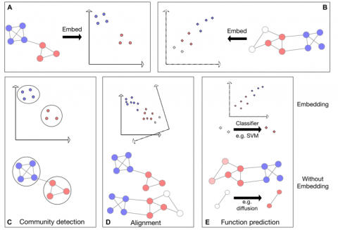
Because of restrictions on servers and network access, dynamic web pages cannot be presented with the same flexibility as static graphics. As a result, one crucial way to visualise shared information is via presenting static graphics. However, compared to web-based visualisation apps, static picture presentation has certain drawbacks. To assist users in delving further into the data content, advanced information visualisation toolkits typically include a variety of interaction modes, including the ability to select a time period, data region, map level, and perform click-and-drag operations. A few instances of interactive information labelling with embedded source code are displayed in Figure 9. Second, Figure 9 (a) shows the initial scenario that interaction can reflect; as Figure 9 (b) illustrates, information cannot be presented properly when the image resolution is low since static images are primarily kept in bitmap format. Third, as demonstrated in Figure 9 (c), the use of a three-dimensional format can help the viewer observe the pattern from various angles, which is not possible with static visualisation images. Fourth, as Figure 9 (d) illustrates, animations are frequently employed in temporal data visualisations to display data from various periods expressed in time steps; Figure 9 (e) shows the predictive performance of the function. A good example is the dynamic map of the world's population and income created by Hans Rosling.
Figure 9. Three examples of applications that incorporate source code into visualisations
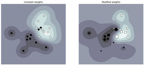
Figure 10. Repositioned colour density map visualization
7.2 Visual repositioning (VR)
For visualisations recorded in a format (like JSON), high-quality visual retargeting can be accomplished without pattern recognition if raw data is encoded as static images using VisCode. We use both representation retargeting and topic retargeting in our implementation. First, we create a static visualisation image in JSON format by encoding the raw data and visualisation type. The data will be shown in the designated type of visualisation image upon decoding. As seen in Figure 10, the user receives an encoded static image as input and an alternative visualisation style as output. Redirecting in this way is known as representational redirection. Second, we may provide consumers with a selection of various colour themes based on pre-existing representations. The term "theme redirection" refers to this colour theme change feature. Rich colour schemes and visual styles can be obtained with this VisCode application. The encoded colour density map can have its raw dispersion data retrieved using VisCode's decoding tool. Figure 10 illustrates an example of a relocated colour density map visualisation. New density maps with customised bandwidths can be created using this scatter data and the kernel density technique.
This paper presents the VisCode model, an encoder-decoder network technique for embedding and extracting hidden information in visualised images. It is possible to incorporate secret information into diagrams and retrieve it using a decoder network by utilising the visual significance network and text transformation model. By reducing interference and incorporating more information into the visualisation design, the suggested VisCode expands the possibilities in the field of data visualisation while enhancing data transmission security and efficiency.
We present a range of techniques in high-dimensional data visualisation to address the problems of data overlap and distribution comprehension. We may more precisely determine the distribution of data by using dithering techniques and Alpha blending algorithms. This is particularly useful when visualising massive amounts of data. In the meanwhile, we may more easily comprehend the general distribution and trends of vast volumes of data by evaluating and charting aggregated information. Lastly, we demonstrate the R big data visualisation tabplot package, which offers a means of classifying data according to particular variables and presenting them in a comprehensible manner. We can learn more about the connections between relevant variables and international students' academic performance by examining and visualising the PISA 2012 dataset.
Overall, by presenting the VisCode paradigm and a range of data visualisation techniques, this study shows some creative advancements in the field of information visualisation. We will keep looking at new visualisation tools and approaches in the future to handle the volume and complexity of data that is growing, as well as to increase the efficacy and efficiency of data analysis.
[1] Tejedor-García, C., Escudero-Mancebo, D., Cámara-Arenas, E., González-Ferreras, C., Cardeñoso-Payo, V. (2020). Assessing pronunciation improvement in students of English using a controlled computer-assisted pronunciation tool. IEEE Transactions on Learning Technologies, 13(2): 269-282. https://doi.org/10.1109/TLT.2020.2980261
[2] Pourhosein Gilakjani, A., Rahimy, R. (2020). Using computer-assisted pronunciation teaching (CAPT) in English pronunciation instruction: A study on the impact and the Teacher’s role. Education and information technologies, 25(2): 1129-1159. https://link.springer.com/article/10.1007/s10639-019-10009-1.
[3] Lan, E.M. (2022). A comparative study of computer and mobile-assisted pronunciation training: The case of university students in Taiwan. Education and Information Technologies, 27(2): 1559-1583. https://link.springer.com/article/10.1007/s10639-021-10647-4.
[4] Rogerson-Revell, P.M. (2021). Computer-assisted pronunciation training (CAPT): Current issues and future directions. RELC Journal, 52(1): 189-205. https://doi.org/10.1177/0033688220977406
[5] Saleh, A.J., Gilakjani, A.P. (2021). Investigating the impact of computer-assisted pronunciation teaching (CAPT) on improving intermediate EFL learners’ pronunciation ability. Education and Information Technologies, 26: 489-515. https://link.springer.com/article/10.1007/s10639-020-10275-4.
[6] Asrifan, A., Zita, C.T., Vargheese, K.J., Syamsu, T., Amir, M. (2020). The effects of call (computer assisted language learning) toward the students’ English achievement and attitude. Journal of Advanced English Studies, 3(2): 94-106.
[7] Xiao, W., Park, M. (2021). Using automatic speech recognition to facilitate English pronunciation assessment and learning in an EFL context: Pronunciation error diagnosis and pedagogical implications. International Journal of Computer-Assisted Language Learning and Teaching (IJCALLT), 11(3): 74-91. https://doi.org/10.4018/IJCALLT.2021070105
[8] Cengiz, B.C. (2023). Computer-assisted pronunciation teaching: An analysis of empirical research. Participatory Educational Research, 10(3): 72-88. https://doi.org/10.17275/per.23.45.10.3
[9] Ulangkaya, Z.K. (2021). Computer assisted language learning (CALL) activities and the students’ English oral proficiency. Randwick International of Education and Linguistics Science Journal, 2(3): 307-314. https://doi.org/10.47175/rielsj.v2i3.301
[10] Bozorgian, H., Shamsi, E. (2020). Computer-assisted pronunciation training on Iranian EFL learners’ use of suprasegmental features: A case study. Computer-Assisted Language Learning Electronic Journal, 21(1): 93-113. https://old.callej.org/journal/21-2/Bozorgian-Shamsi2020.pdf.
[11] Sabir, I.S., Afzaal, A., Begum, G., Sabir, R.I., Ramzan, A., Iftikhar, A. (2021). Using computer assisted language learning for improving learners linguistic competence. Multicultural Education, 7(4): 81-94. http://ijdri.com/me/wp-content/uploads/2021/04/9.pdf.
[12] Enayati, F., Gilakjani, A.P. (2020). The impact of Computer assisted language learning (CALL) on improving intermediate EFL learners' vocabulary learning. International Journal of Language Education, 4(1): 96-112. https://doi.org/10.26858/ijole.v4i2.10560
[13] Chidananda, K., Kumar, A.P.S. (2023). A robust multi descriptor fusion with One-Class CNN for detecting anomalies in video surveillance. International Journal of Safety and Security Engineering, 13(6): 1143-1151. https://doi.org/10.18280/ijsse.130618
[14] Reda, N.H., Abbas, H.H. (2024). 3D human facial traits’ analysis for ethnicity recognition using deep learning. Ingénierie des Systèmes d’Information, 29(2): 501-514. https://doi.org/10.18280/isi.290211
[15] Jiang, Y., Chun, D. (2023). Web-based intonation training helps improve ESL and EFL Chinese students' oral speech. Computer Assisted Language Learning, 36(3): 457-485. https://doi.org/10.1080/09588221.2021.1931342
[16] Hanon, W., Salman, M.A. (2024). Integration of ML techniques for early detection of breast cancer: Dimensionality reduction approach. Ingénierie des Systèmes d’Information, 29(1): 347-353. https://doi.org/10.18280/isi.290134
[17] Hussein, S.S., Rashidi, C.B.M., Aljunid, S.A., Salih, M.H., Abuali, M.S., Khaleel, A.M. (2023). Enhancing cardiac arrhythmia detection in WBAN sensors through supervised machine learning and data dimensionality reduction techniques. Mathematical Modelling of Engineering Problems, 10(6): 2051-2062. https://doi.org/10.18280/mmep.100615
[18] Ramsankar, A.D., Krishnamoorthy, A. (2024). Exploring metric dimensions for dimensionality reduction and navigation in rough graphs. Mathematical Modelling of Engineering Problems, 11(4): 1037-1043. https://doi.org/10.18280/mmep.110421
[19] Tseng, W.T., Chen, S., Wang, S.P., Cheng, H.F., Yang, P.S., Gao, X.A. (2022). The effects of MALL on L2 pronunciation learning: A meta-analysis. Journal of Educational Computing Research, 60(5): 1220-1252. https://doi.org/10.1177/07356331211058662
[20] Mohsen, M.A., Mahdi, H.S. (2021). Partial versus full captioning mode to improve L2 vocabulary acquisition in a mobile-assisted language learning setting: Words pronunciation domain. Journal of Computing in Higher Education, 33(2): 524-543. https://link.springer.com/article/10.1007/s12528-021-09276-0.
[21] Sadiq, A.H.B., Razaq, H.R., Mustafa, K. (2023). Tutoring speech organs with computer-assisted language learning. Jahan-e-Tahqeeq, 6(3): 95-107. https://www.jahan-e-tahqeeq.com/index.php/jahan-e-tahqeeq/article/view/915.
[22] Chatterjee, S. (2022). Computer assisted language learning (CALL) and mobile assisted language learning (MALL); Hefty tools for workplace English training: An empirical study. International Journal of English Learning & Teaching Skills, 4(2): 1-7. https://doi.org/10.15864/ijelts.4212
[23] Kruk, M., Pawlak, M. (2023). Using internet resources in the development of English pronunciation: The case of the past tense-ed ending. Computer Assisted Language Learning, 36(1-2): 205-237. https://doi.org/10.1080/09588221.2021.1907416
[24] Tejedor-García, C., Escudero-Mancebo, D., Cardeñoso-Payo, V., González-Ferreras, C. (2020). Using challenges to enhance a learning game for pronunciation training of English as a second language. IEEE Access, 8: 74250-74266. https://doi.org/10.1109/ACCESS.2020.2988406
[25] Detey, S., Fontan, L., Le Coz, M., Jmel, S. (2020). Computer-assisted assessment of phonetic fluency in a second language: A longitudinal study of Japanese learners of French. Speech Communication, 125: 69-79. https://doi.org/10.1016/j.specom.2020.10.001
[26] Zhang, C., Li, M., Wu, D. (2022). Federated multidomain learning with graph ensemble autoencoder GMM for emotion recognition. IEEE Transactions on Intelligent Transportation Systems, 24(7): 7631-7641. https://doi.org/10.1109/TITS.2022.3203800