Ning Ma![]() | Songwen Jin*
| Songwen Jin*![]() | Yanming Zhao
| Yanming Zhao![]()
© 2024 The authors. This article is published by IIETA and is licensed under the CC BY 4.0 license (http://creativecommons.org/licenses/by/4.0/).
OPEN ACCESS
At this stage, the 3D graph convolution algorithm has the following problems: (1) Neighbor space selection problem; (2) Feature extraction and fusion problem of different depth map convolution algorithms; (3) Multi-view parallel feature fusion problem. Based on this, "Multi-domain adaptive graph convolution algorithm based on visual computing theory and its scene segmentation application" is proposed. First, inspired by the 3D vision of primates, a 3D visual computing theory is proposed; and propose an adaptive graph convolution algorithm based on the 3D visual selectivity theory. It solves the problem of neighbor space selection for 3D graph convolution; secondly, inspired by the single-link serial processing mode of primate visual information, a single-link depth adaptive graph convolution algorithm based on 3D visual selectivity is constructed to learn and refuse the different depth visual features of the same sub-space of 3D point cloud; Finally, inspired by the multi-link parallel processing model of primate visual information, we improved the single-link algorithm and constructed a multi-link depth adaptive graph convolution algorithm based on 3D visual selectivity to learn and integrate global visual features of different link; and using the MLP algorithm with shared weights to achieve object segmentation.On ShapeNetPart and custom Mortise_and_Tenon_DB, Compare with PointNet, PointNet++, KPConv deform, 3D GCN and other algorithms. Verify the segmentation performance and geometric invariance of this algorithm. The experimental results: The segmentation performance of the algorithm of this article is good, and the segmentation success rate reaches 90.9%; the algorithm of this article has strong geometric invariance, Rotation and translation transformations are geometrically invariant, and Scaling transformation has finite geometric invariance in the interval [-0.15,0.15].
visual selectivity, graph convolution, multi-view, visual information processing pattern, information fusion
Breakthroughs in 3D sensor technology [1] that overcome the precision bottleneck of point cloud collection can capture accurate point cloud datasets, providing a data foundation for the rapid advancement of 3D point cloud data processing algorithms. These advancements have achieved good research and application results in fields such as drone control [2], autonomous driving [3], augmented reality [4], and medical image processing [5].
Conventional convolution algorithms based on 2D structured spaces cannot be directly applied to semi-structured 3D point cloud spaces. Based on this, researchers have proposed point cloud space structuring algorithms, direct point cloud processing algorithms, and direct structuring algorithms to address the issue of spatial feature extraction in semi-structured spaces.
Point cloud space structuring algorithms essentially solve the problem of structuring 3D point cloud data by structuring 3D point cloud space, facilitating the direct or expanded application of two-dimensional convolution methods to this 3D structured space. The main methods include: voxel-based approaches [6-8] and multi-view methods [9-11]. However, the structuring algorithms for 3D point cloud data have the following shortcomings: (1) Structuring of 3D space results in overlap of some data, compromising the purity and completeness of the original data points. (2) The process of structuring 3D space increases the complexity of the algorithms and reduces their performance. (3) Polarized structuring (such as the view method) loses three-dimensional topological structure information, affecting the recognition performance of the algorithms.
Therefore, direct point cloud processing algorithms have been proposed, which do not require structuring of 3D point cloud datasets and perform feature learning directly on the original datasets, attempting to address the aforementioned shortcomings. These include: PointNet [12], PointNet++ [13], and subsequent improvements to these algorithms [14-16].
Practice has shown that structured information expressed by spatial topological structure is an essential feature of 3D point clouds, and neither spatial structuring algorithms nor direct point cloud processing methods can effectively solve the learning and representation of 3D point cloud spatial structuring information. Graph structure is an excellent way to learn and represent spatial structuring information. Thus, the graph convolution method has become a direction for 3D point cloud research [17-20], achieving certain research and application progress.
The Dynamic Graph Convolutional Neural Network (DGCNN) algorithm [21] constructs local graph structures by identifying the nearest neighbors of 3D points in feature space and then performing edge convolution operations to extract features. Shen et al. [22] extended this idea and further learned spatial topological information during the feature aggregation process. Relation-Shape Convolutional Neural Network (RS-CNN) [23] applies the weighted sum of neighboring node features, where each weight is learned using an MLP based on the geometric relationship between the two points. These efforts aim to learn the local topological features of three-dimensional point clouds. 3D-GCN [24] uses a deformable 3D kernel to learn information from 3D point clouds and addresses the disorder and unstructured nature of point cloud data through graph-based max pooling methods, proposing a universal model concept. The GCN algorithm based on visual selectivity [25] proposes a method that combines point cloud information with point cloud topological structure features, establishing a graph convolution computation method. It effectively solves the problem of learning and integrating global and local features. The multi-view depth-adaptive GCN [26] method, integrating visual computing techniques with GCN algorithms, addresses the inability of existing GCNs to effectively learn the correlation between different scale visual features under multi-view (multi-domain) conditions. Point cloud transformer [27] presents a novel framework named Point Cloud Transformer (PCT) for point cloud learning. PCT is based on Transformer, which achieves huge success in natural language processing and displays great potential in image processing. TransNet [28] proposes a novel downsampling model based on the transformer-based point cloud sampling network (TransNet) to efficiently perform downsampling tasks. The proposed TransNet utilizes self-attention and fully connected layers to extract meaningful features from input sequences and perform downsampling.
Despite the theoretical and practical research achievements in 3D point cloud processing through GCN methods, there are still shortcomings: (1) The selection of neighboring space for graph convolution and spatial selection for information aggregation lacks theoretical support. (2) How to integrate features at different scales in deep graph convolution algorithms. (3) The algorithms do not utilize multi-view information for parallel fusion models, achieving parallel extraction and fusion of visual features, which results in single visual feature structures, weak correlations, and low classification accuracy.
Based on this, this study proposes an adaptive GCN algorithm based on visual computing theory and discusses its application in scene segmentation. The paper expands the theory of 2D visual selectivity to form a theory of 3D visual selectivity and proposes an adaptive graph convolution algorithm based on 3D visual selectivity (abbreviated as AGCNTDVS). Combining this algorithm with deep learning theory, we form a single-linkage depth-adaptive GCN algorithm based on 3D visual selectivity (abbreviated as SD-AGCNTDVS), which extracts visual features at different depths and effectively integrates them. Inspired by the parallel visual information processing pattern of primates, building on the single-linkage algorithm, we construct a multi-linkage deep adaptive GCN algorithm based on 3D visual selectivity (abbreviated as MD-AGCNTDVS), extracting and optimizing visual features from different linkages.
Therefore, the innovations of this paper include:
(1) Theoretically, inspired by the 3D vision of primates [29], we propose a theory of 3D visual computation. Based on 3D spatial visual selectivity, we propose the AGCNTDVS algorithm, which addresses the issues of spatial partitioning and information aggregation in graph convolution, and adaptively learns the global and local features of 3D point clouds.
(2) Inspired by the serial visual information processing pattern of primates, we integrate the AGCNTDVS algorithm with deep graph convolution learning theory to construct a SD-AGCNTDVS algorithm, which learns deep abstract features of 3D point clouds at various depths and achieves feature integration.
(3) Inspired by the parallel visual information processing pattern of primates [30], and using viewpoints as a standard, we expand the SD-AGCNTDVS algorithm to construct the MD-AGCNTDVS algorithm to learn multi-linkage features, forming a feature fusion matrix, and representing the optimal visual area.
(4) We apply this algorithm to the custom Mortise_and_Tenon_DB dataset for the digital reconstruction of the joint structure, achieving adaptive segmentation of mortise and tenon structures. This validates the correctness of the structural segmentation and provides effective support for the intelligent design of ancient Chinese buildings.
2.1 Theory of visual selectivity in 3D space
The visual selectivity of primates indicates that the function of visual cells is characterized by "like attracts like, differences repel", expressed through the receptive fields of visual neurons. Based on this, the theory of 3D visual selectivity is proposed: (1) In 3D space, the visual selectivity of visual cells also follows the characteristic of "like attracts like, differences repel"; (2) It is represented through the 3D receptive field (spatial topological structure) of points, i.e., the intrinsic characteristics of a point and its spatial structure with neighboring points, which is invariant. (3) Based on the above points (1) and (2), by dividing according to the function of the receptive field, 3D visual space can be partitioned, and this partitioning has a reasonable basis in visual physiology theory.
2.2 Theory of 3D graph convolution and its computational methods
Research on GCN based on spatial maps describes graph convolution as a method of aggregating features from neighbors, including three steps: classification, aggregation, and activation.
Spatial Classification: Inspired by the theory of 3D visual selectivity, a clustering segmentation algorithm is used to perform spatial division of the 3D GCN algorithm, dividing the $3 \mathrm{D}$ point cloud space, $\Omega$, into $\mathrm{K}$ subspaces, i.e., $\Omega=$ $\cup_{k=1}^K \Omega_k\left(o_k, R_k\right)$, and $\bigcap_{k 1=1}^K \Omega_k\left(o_{k 1}, R_{k 1}\right)=\Phi$, while $k 1 \neq k$. Each subspace $\Omega_k\left(o_{k 1}, R_{k 1}\right)$ contains points with simila receptive fields.
Therefore, the receptive field in $3 \mathrm{D}$ visual space is defined as: When $q \in \Omega_k\left(o_k, R_k\right)$, the receptive field of point includes two parts of information: the information of point and the spatial structural relationship between $q$ and neighboring nodes in $\Omega_k\left(o_k, R_k\right)$, expressed as:
$\left\{\begin{array}{c}\operatorname{TDRF}_q\left(o_k, R_k\right)=\left\{(\text { inform_feature }(q), \text { toplogical_feature }(q)) \mid \forall q \in \Omega_k\right\} \\ \text { inform_feature }(q, t)=(x, y, z, \varphi, \text { other_global_feature }), q \in \Omega_k \text { and dist }(\mathrm{p}, \mathrm{q})<\varepsilon \\ \text { topological_feature }(q)=\Phi\left(\left(\alpha, \beta, \gamma, \rho, \Delta, w_i^{j k}\right)_{m n}\right) \\ \Omega_k\left(o_k, R_k\right)=M_P(R)=M_i^j(R)=\left\{P_j \mid\left\|P_j-P_i\right\| \leq R, i, j=1,2,3, \ldots\right\}\end{array}\right.$ (1)
Here, $\Omega_k\left(o_k, R_k\right)$ represents a hypersphere in visual space with center $o_k$ and radius $R_k$. In $\Omega_k$, visual cells have the same or similar functions and stable spatial structures.
In the visual space $\Omega_k$, the information (global attributes) features of observation point $\forall p_i \in \Omega_k$ are represented as: $(x, y, z, \varphi$,other_global_feature), where $x, y, z$ denote the global spatial location of point $p_i$, parameter $\varphi$ represents the number of topological divisions in the global visual space; other_global_feature indicates other global spatial features of the point, such as curvature and normal vectors.
In the visual space $\Omega_k\left(o_k, R_k\right)$, the spatial topological information of observation point $p_j$ is represented as $\left(\alpha, \beta, \gamma, R, w_i^{j k}\right)$, where parameters $\alpha, \beta, \gamma, R$ describe the local visual topological structure of the observation point $p_j$, where azimuth angles $\alpha, \beta, \gamma$ respectively represent the local topological structure parameters of the visual space of vector $\overrightarrow{P_l P_j} ; R$ is the magnitude of vector $\overrightarrow{P_l P_j}$, representing the spatial distribution range of this vector. Parameter $w_i^{j k}$ represents the minimum or sub-minimum number of points forming a stable local visual structure in the visual space $\Omega\left(R, P_i\right)$, referred to as the richness of the receptive field; matrix $\left(\alpha, \beta, \gamma, \rho, \Delta, w_i^{j k}\right)_{m n}$ represents the local spatial topological set of observation point $p_j$, which learns the essential features of the set through mapping $\Phi$, with these features being stable. In this paper, $\Phi=M L P$.
Therefore, the spatial receptive field $T D R F_q\left(o_k, R_k\right)$ is an integration of local and global features, which better learns and expresses the visual information of 3D point clouds; here, when $\lim \left(\left\|\overrightarrow{P_2 P_j}\right\| / R\right) \rightarrow o(0)$, the points in the visual space $\Omega\left(o_k, R_k\right)$ have stable and similar receptive fields, forming a smaller receptive field space through clustering.
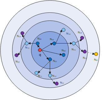
Thus, according to the above definitions, the $3 \mathrm{D}$ point cloud space receptive field and the graph convolution algorithm are described as Figure 1.
(a) Global Ω space of the point cloud
(c) K-nearest neighbor relationships of point $p$ in $\Omega_k\left(o_k, R_k\right)$
(d) Spatial structure $T D R F(p, R)$ of the subspace $\Omega_k\left(o_k, R_k\right)$
Figure 1. Space of three-dimensional point clouds and their graph convolution
2.3 Theory of 3D visual information processing links
The visual information processing of primates includes both serial and parallel modes, which are deeply integrated to form optimal visual information features. Based on this, a single-linkage hierarchical serial visual information processing mode and a multi-linkage parallel processing mode based on a single link are formed in the theory of visual computation. The single-linkage hierarchical serial visual information processing mode can complete the extraction and integration of the same visual information at different depths, and it has a strong capability for deep feature abstraction learning for deep learning of visual information [27-29], but it lacks dependency learning of visual information. The multi-linkage parallel processing mode, created based on the single-linkage hierarchical serial visual information processing mode, achieves deep integration of multiple single-linkage visual information, implements inter-linkage feature dependency learning, and extracts the integrated features of information from different visual links. This solves the dependency of visual features and enhances the expressive power of visual features.
Based on the theoretical analysis mentioned above, this paper proposes and implements three algorithms: AGCNTDVS, SD-AGCNTDVS, and MD-AGCNTDVS.
3.1 The AGCNTDVS
Inspired by the theory of 3D visual space selectivity, this algorithm integrates 3D visual selectivity with graph convolution algorithms, proposing the AGCNTDVS. The main steps of AGCNTDVS include spatial selection, information aggregation, and activation, detailed as follows.
(a) K-nearest neighbor clustering space division diagram
(b) Graph convolution information aggregation diagram
Figure 2. Information aggregation method of graph convolution based on visual selectivity
(1) Spatial Selection
Inspired by the theory of 3D visual selectivity, the selection process mainly targets the global visual space $\Omega$, utilizing the K-means clustering method to achieve the subdivision of the global space into subspaces, denoted as $\Omega=\bigcup_{k=1}^{k=K} \Omega_k\left(o_k, R_k\right)$ Elements within $\Omega_k$ have the same or similar functions (receptive fields).
(2) Information Aggregation
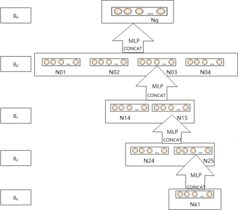
In the visual subspace $\Omega_k\left(o_k, R_k\right)$, for $\forall q \in \Omega_k$, the spatial topological information of observation point $q$ and its Lnearest neighborhood $\Omega_{\text {Neighbor }}\left(R_L, q\right), L=0,1,2, \ldots,, K$ is represented as vector $\mu=\left(\alpha, \beta, \gamma, R, w_i^{j k}\right)$. In this paper, the function $\Phi=$ MLP, meaning a MLP is used to learn the spatial topological structure between neighbors (Figure 2). Therefore, the information aggregation of observation point $q$ and its neighborhood $\Omega_{\text {Neighbor }}\left(R_L, q\right)$ are represented as:
$\begin{gathered}\text { topological_Feature }\left(R_i, q\right)= \\ \operatorname{MLP}\left(\operatorname{CONCAT}\left(\left(\operatorname{MAP}\left(R_i, N_0^j\right), j=\right.\right.\right. \\ \left.\left.\left.1,2,3 \ldots, \text { nember }\left(\Omega_{\text {Neighbor }}\left(R_L, q\right)\right),\right)\right)\right)\end{gathered}$ (2)
$\begin{gathered}\operatorname{MAP}\left(R_i, N_i^j\right)= \\ \operatorname{MLP}\left(\operatorname{CONCAT}\left(\left(\operatorname{MAP}\left(R_{i-1}, N_{i-1}^j\right), j=\right.\right.\right. \\ \left.\left.\left.1,2,3 \ldots, \operatorname{nember}\left(\Omega_{\text {Neighbor }}\left(R_L, q\right)\right)\right)\right)\right)\end{gathered}$ (3)
Inspired by visual selectivity theory, topological_Feature has a stable number of points and stable spatial structure, and for $\forall \mathrm{q} \in \Omega_k\left(o_k, R_k\right)$, point $q$ has a stable number of points and structure, which is independent of the input point order.
(3) Activation
To increase the non-linearity of the features, the algorithm uses the ReLU(R) activation function, with different pooling radii used for different visual areas.
The pseudocode for the AGCNTDVS algorithm is shown in Table 1.
Table 1. Pseudocode for the AGCNTDVS algorithm
|
Input: point cloud data $(\Omega)$; hyperparameter $R$; observation point $p$ |
|
Produce: S1: Selection and k-nearest neıghbor initıalızation. On the global point cloud visual space $\Omega$, execute the K-means clustering algorithm, $\cup_{k=1}^{k=K} \Omega_k(R, p)=R F K N N(\Omega)$, and $\bigcap_{k=1}^{k=K} \Omega_k(R, p)=$ $\Phi, \forall q \in \Omega_k(R, p)$, initialize the k-th order neighbor space $\Omega_{\text {Neighbor }}(q, k)$ and its virtual edge structure (for specifying neighbor relationships) based on "closest distance most similar function". $t_1=1, k=1$. S2: Feature selection and aggregation. On the neighborhood $\Omega\left(R_L, q\right)$ of point $q$, perform feature selection and aggregation through iterations of features corresponding to neighborhoods from $R_0$ to $R_K$ using Formulas (2) and (3). S3: Activation. Perform RELU(R) activation on aggregated features to increase the non-linearity of the features. S4: If $t_1 \leq\left\|\Omega_k(R, p)\right\|$, the algorithm goes back to step S2; otherwise, after completing 3D graph convolution calculations for $\Omega_k(R, p)$, proceed to step $\mathrm{S} 5$. S5: If $\mathrm{k} \leq \mathrm{K}$, the algorithm returns to step S2; otherwise, after completing 3D graph convolution calculations for the global point cloud visual space $\Omega$, the algorithm ends. |
|
Output: Graph convolution Local_feature $(p)$ of point $p$ in the neighborhood $\Omega_k(R, p)$ and the set of clustering radii $\{\mathrm{r}\}$. |
3.2 The SD-AGCNTDVS
Table 2. Pseudocode for the SD-AGCNTDVS algorithm
|
Input: point cloud data $(\Omega)$; hyperparameter R; observation point $P_i$; Network depth parameter L. |
|
Produce: S1: Parameter Initialization. Initialize the network depth parameter Net_Deep_Len $=1$; select observation set $\Omega_k\left(R, p_i\right) \subset \Omega$ S2: 3D Visual Depth Calculation. In the 3D visual set $\Omega_k\left(R, P_i\right)$, sequentially execute the AGCNTDVS. The process involves: AGCNTDVS ${ }^{\text {Net_Deep_Len }+1}=$ AGCNTDVS ${ }^{\text {Net_Deep_Len }}\left(\Omega_k\left(R, P_i\right)\right) \quad, \quad$ incrementing Net_Deep_Len by 1, and linking the generated features of different layers in sequence. S3: If Net_Deep_ Len $\leq \mathrm{L}$, the algorithm loops back to step S2. Otherwise, the SD- AGCNTDVS algorithm ends, and deep feature extraction is complete. |
|
Output: Output features formed by linking visual features at different depths. |
Inspired by the serial processing mode of 3D visual information, this paper integrates the AGCNTDVS algorithm with deep learning theory to construct the SD-AGCNTDVS. The AGCNTDVS algorithm extracts abstract visual features of the 3D point cloud from different depths and merges these features to form complex visual features, enhancing the capability of the algorithm to extract visual features and enriching the expression of visual features. Thus, the pseudocode for the SD-AGCNTDVS is shown in Table 2.
3.3 Semantic segmentation algorithm based on SD-AGCNTDVS
Use the SD-AGCNTDVS algorithm for semantic segmentation of three-dimensional point cloud data, achieving multi-scale feature aggregation of the $3 \mathrm{D}$ point cloud collection and using a per-point classification shared MLP algorithm. Since the algorithm uses a pooling mechanism, the feature lengths of three-dimensional point cloud data between different layers do not match. Based on this, the following feature filling operation, the Fill_algorithm, is defined:
$\text { Fill }_{\text {algorithm }}=T D E F_q(p, R)= \\
\operatorname{argmin}\left(T D E F_{\bar{q}, r}(p, R)\right), \text { and } \bar{q} \in \dot{U} U(q, r)$ (4)
Here, $q$ is the point to be filled, and $\dot{U}(q, r)$ represents the punctured r-neighborhood of point $q$.
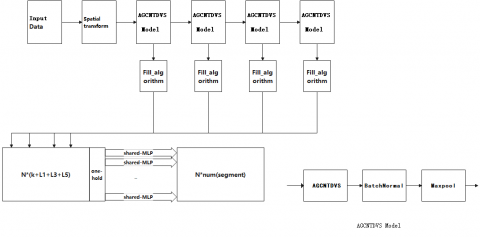
Thus, the model for the semantic segmentation algorithm based on the SD-AGCNTDVS (abbreviated as SSMAGCNTDVS) is given below (Figure 3).
(1) Traditional segmentation algorithms
Figure 3. The 3D SSM-AGCNTDVS model based on the AGCNTDVS algorithm
3.4 The MD-AGCNTDVS
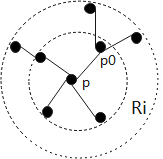
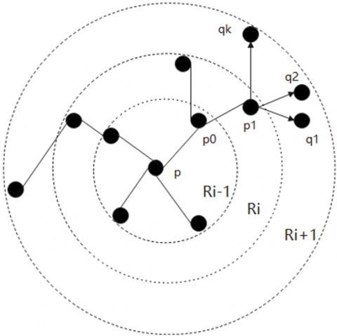
The AGCNTDVS extracts deep visual features of the 3D point cloud; it has not studied the breadth visual features of the 3D point cloud and the correlation of its breadth features. The clustering radius r of the AGCNTDVS algorithm determines the learning of breadth features and the analysis and application of feature correlations, with a microscopic analysis as shown in Figure 4.
The above figure shows that different visual neighborhoods $R$ correspond to different neighborhoods of point $p$; on different neighborhoods, the features of point $p$ aggregated by the AGCNTDVS algorithm vary; when $R$ is too small, the visual region $\Omega_q(R, p)$ of point $p$ is too small, leading to insufficient expressive regions for the graph convolution, resulting in poor completeness; when $R$ is too large, the visual region $\Omega_q(R, p)$ is too large, containing different functional cells, and the visual information within the region does not satisfy visual selectivity, resulting in poor purity of visual features extracted from the $\Omega_k\left(R, P_i\right)$ collection; therefore, the hyperparameter $R$ is set during the experimental process.
Based on this, this paper proposes the MD-AGCNTDVS, which adaptively extracts features within several consecutive visual regions corresponding to different $R$ values, to learn the optimal or suboptimal global and local spatial features, addressing the shortcomings of the SD-AGCNTDVS algorithm. The pseudocode for the MD-AGCNTDVS is shown in Table 3.
a) $R_{i-1}$ order visual region
b) $R_i$ order visual region
c) $R_{i+1}$ order visual region
Figure 4. Microscopic relationship between visual regions and feature extraction by the 3D GCN algorithm
Table 3. Pseudocode for the MD-AGCNTDVS algorithm
|
Input: point cloud data $(\Omega(R, p)$; hyperparameter set $\mathrm{R}$; observation point $p$ (set $p$ is the triplet of continuous natural number); Network depth parameter L. |
|
Produce: S1: Algorithm Initialization: Based on the hyperparameter $R$, generate neighborhoods $\Omega\left(R_1, p\right), \Omega\left(R_2, p\right), \ldots, \Omega\left(R_{N 0}, p\right)$, where $R_1 \leq R_2 \leq \cdots \leq R_{N 0}$ S2: Multi-feature learning: Start multiple GPUs or threads to parallelly learn visual features from different visual regions $\Omega\left(R_i, p\right)$ : $\operatorname{TDEF}\left(p, R_i\right)=$ Single link deep AGCNTDVS $\left(\Omega\left(R_i, p\right)\right)$ S3: Multi-domain feature fusion learning: $H\left(T D E F\left(p, R_{-} i\right)\right)$, where $H(\cdot)$ is a feature fusion function. |
|
Output: Output different depth visual features and their fusion features. |
3.5 Application model of MD-AGCNTDVS for 3D point cloud segmentation
The function H(·) fuses the segmentation results of the multi-domain adaptive GCN algorithm based on visual computing theory. In this paper's experiments, it can be implemented using an MLP algorithm, or through algorithms like MaxPool.
$\begin{aligned} & H(.)=\operatorname{MLP}\left(\operatorname{MDDVSA3DGCN}\left(\mathrm{R}_i\right)\right) \\ & \text { or } \operatorname{MaxPool}\left(\operatorname{MDDVSA3DGCN}\left(R_i\right)\right)\end{aligned}$ (5)
Here, the MaxPool algorithm learns the global maximum of different visual region features, representing global features and ignoring the details of features, with a lower time complexity. Meanwhile, the MLP algorithm learns the fused features of different visual regions, including the correlation between various features, hence, the features are more representative, but the feature fusion has higher time complexity.
3.6 Algorithm invariance
Existing works such as [14, 21, 23, 26, 31-34] have reported good geometric invariance performance, but they typically consider global coordinates or require point cloud normalization to mitigate this data variation, which could limit their invariance. The algorithm in this paper learns directional information and its directional selectivity within local receptive fields through 3D convolution kernels, and these features are formed independently of specific positions and distances, further enhanced by pooling mechanisms to improve the algorithm’s geometric invariance. Therefore, the algorithm exhibits good translational, scale, and rotational invariance.
4.1 Dataset
To verify the 3D object segmentation capability of the algorithm in this paper, the ShapeNetPart dataset [35] was used as the validation database, consisting of 16,881 CAD models of 16 object types, with each point in an object corresponding to a part label. There are a total of 50 categories, with each object type having 2 to 6 part categories available. For comparison with traditional algorithms, this experiment extracted 1024 points from each 3D model for training and testing.
4.2 Evaluation method
This paper uses the mean Intersection over Union (mIoU) to assess segmentation performance, which is the average IoU for each part type within the object category.
IoU is a concept used in object detection. IoU calculates the overlap rate between the "predicted bounding box" and the "actual bounding box"—that is, the ratio of their intersection to their union. The ideal situation is complete overlap, i.e., the ratio is 1.
$\operatorname{IoU}\left(S_{\text {Predict }}, S_{\text {True }}\right)=\frac{S_{\text {Predict }} \cap S_{\text {True }}}{S_{\text {Predict }} \cup S_{\text {True }}}$ (6)
Meanwhile, the mIoU is the average of the IoUs for all shape instances within that object category, expressed as:
$m I o U=\frac{1}{N} \sum_{i=1}^N I o U(i)$ (7)
Here, N represents the number of instances in the object, and in this experiment, N = 16.
4.3 Network configuration
The model architecture is shown in Figure 5. The feature extraction part consists of 5 layers, with kernel numbers (2, 3, 5, 7, 9) at relevant layers, and two 3D Graph Max pooling layers deployed with a fixed sampling rate r=6. Features for segmentation are formed by connecting features from layer outputs at different scales; an additional one-hot vector indicates the object type connected to the aforementioned features; followed by an MLP layer that fuses multi-link visual features based on the generated fusion feature. A shared-weight MLP layer is used to classify each point's segmentation label. We trained our algorithm using the ADAM optimizer with a learning rate of 0.001, decaying by half every 10 epochs.
4.4 Comparative experiment of algorithms
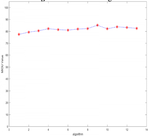
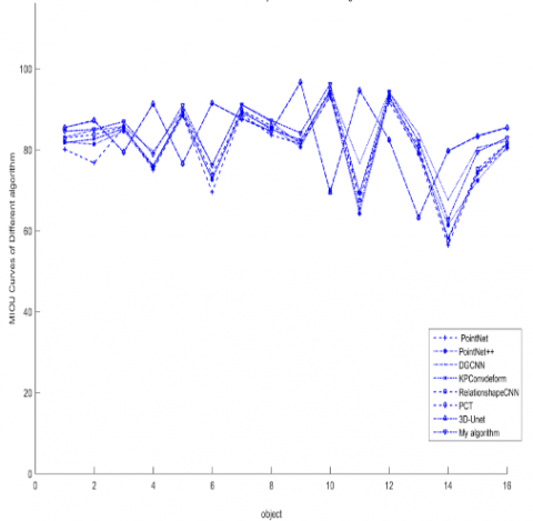
On the ShapeNetPart dataset, using mIOU as the evaluation standard and employing the network parameters set in Section 4.3, a comparative experiment between the MD-AGCNTDVS algorithm and traditional algorithms was conducted, and the results are shown in Figure 6.
Figure 5. Semantic segmentation network for 3D point cloud based on MD-AGCNTDVS
(a) MIOU curves of different algorithms
(b) MIOU curves of different algorithms for the same object
(c) MIOU of the different object
(d) Relationship curves between objects, algorithms and MIOU value
Figure 6. Relationship curves between objects, algorithms and MIOU value on the ShapeNetPart dataset
Experimental results show that on the ShapeNetPart dataset, when compared with algorithms such as Kd-Net [32], MRTNet [33], PointNet [12], KCNet [34], RS-Net [23], SO-Net [35], PointNet++ [13], DGCNN [21], KPConv deform [36], Relation shape CNN [37], PCT [27] ,3D-Unet [28] and myalgorithm and, our algorithm achieved segmentation results that are comparable to or better than the most recent methods, this proves that our algorithm is correct and feasible, and it possesses significant algorithmic advantages.
4.5 Validation of geometric invariance
On the ShapeNetPart dataset, and using mIOU as the evaluation standard, the geometric invariance of the MD-AGCNTDVS algorithm was validated with the network parameters set in Section 4.3 (Table 4).
Table 4. Geometric invariance performance comparison table
|
Object |
GT |
KPConv [25] |
Shift |
Scaling |
PointNet++ [13] |
Shift |
Scaling |
|
Airplan |
|
||||||
|
chair |
|||||||
|
Motorbike |
|
|
|||||
|
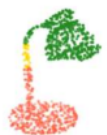
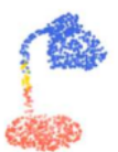
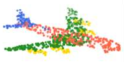
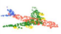
Lamp |
|
|
|||||
|
Object |
GT |
3D GCN [24] |
shift |
scaling |
My paper |
shift |
scaling |
|
Airplan |
|
|
|
|
|||
|
chair |
|
|
|||||
|
Motorbike |
|
|
|||||
|
Lamp |
|
|
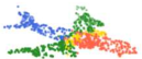
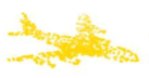
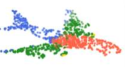
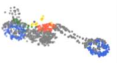
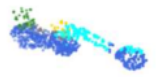
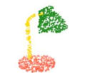
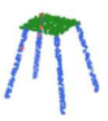
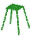
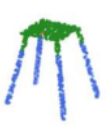
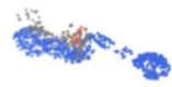
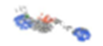
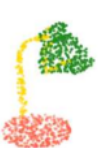
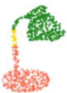
Experiments demonstrate that on the ShapeNetPart dataset for part segmentation visualization, the segmentation outputs of our algorithm were compared with those from KPConv [34], PointNet++ [23], and 3D GCN [24]. It showed that our algorithm possesses good geometric invariance. Here, GT (Ground Truth) represents the true part labels on the ground.
4.6 Experiments on traditional Chinese architectural mortise and tenon structure object segmentation
Mortise and tenon structures are fundamental elements of traditional Chinese architecture. According to the functional needs of the building, traditional Chinese architectural support structures are optimized combinations of several mortise and tenons and Dougong structures, forming a perfect mechanical support structure. Thus, the mortise and tenon structure and its application research are important research areas in traditional Chinese architecture and play a significant role in the development of Chinese architecture. To verify the capability of our algorithm in segmenting traditional Chinese architectural mortise and tenon structures, traditional Chinese architecture includes 32 common types of mortise and tenon structures. This project selected 16 types of mortise and tenon structures to form the 3D point cloud database Mortise_and_Tenon_DB, which serves as the validation database. This dataset consists of 15,330 CAD models of 16 object types, with each point in an object corresponding to a part label. For comparison with traditional algorithms, this experiment extracted 1024 points from each 3D model for training and testing.
On the Mortise_and_Tenon_DB dataset, using mIOU as the evaluation standard, and employing the network parameters set in Section 4.3, a comparative experiment was conducted between the MD-AGCNTDVS algorithm and traditional algorithms, and the comparative experiment results are shown in Figure 7.
(a) MIOU curves of different algorithms
(b) MIOU curves of different algorithms for the same object
(c) MIOU of the different object
(d) Relationship curves between objects, algorithms and MIOU value
Figure 7. Relationship curves between objects, algorithms and MIOU value on Mortise_and_Tenon_DB
The results demonstrate that on the Mortise_and_Tenon_DB dataset, when compared with algorithms such as Kd-Net [34], MRTNet [34], PointNet [12], KCNet [22], RS-Net [23], SO-Net [26], PointNet++ [13], DGCNN [36], KPConv deform [25], 3D GCN [24], PCT [27], 3D-Unet [28] and myalgorithm, our algorithm achieved segmentation results that are comparable to or better than traditional methods. This confirms that our algorithm is correct and feasible, and it has considerable algorithmic advantages.
In this experiment, 10 classes were randomly selected from the Mortise_and_Tenon_DB database to verify the geometric invariance of the proposed algorithm, where the scaling transformation was defined as isotropic scaling transformation along three axes; the parameter $\vartheta$ represents the scaling size of the point cloud set, expressed as a percentage relative to the GT model. To truly reflect the impact of the 3D model's own changes during geometric transformations on the algorithm's segmentation performance, we define a geometric transformation evaluation coefficient:
$\rho=\frac{\text { mIOU(Geometric_transformation_object })}{\text { mIOU(mate_object })}$ (8)
Here, eometric_transformation_object represents the mIOU value of a transformed set, and mIOU (mate_object) represents the $\mathrm{mIOU}$ value without geometric transformations; the evaluation coefficient $\rho$ indicates the extent to which which geometric transformations affect the algorithm, with the mIOU calculation method referred to in Formula (X). The results of the geometric invariance experiments are shown in Table 5 and Figures 8 and 9.
Table 5. Results of the geometric invariance experiments
|
Object Name |
PointNet |
PointNet++ |
KPConv deform |
||||||
|
Translation |
Rotation |
Scaling |
Translation |
Rotation |
Scaling |
Translation |
Rotation |
Scaling |
|
|
CST |
0.99 |
1.00 |
0.96 |
0.99 |
1.00 |
0.96 |
0.99 |
1.00 |
0.96 |
|
IST |
0.99 |
1.00 |
0.97 |
0.99 |
1.00 |
0.97 |
0.99 |
1.00 |
0.97 |
|
HHT |
0.99 |
1.00 |
0.95 |
0.99 |
1.00 |
0.95 |
0.97 |
1.00 |
0.95 |
|
WLT |
0.99 |
1.00 |
0.96 |
0.94 |
1.00 |
0.96 |
0.99 |
1.00 |
0.96 |
|
MST |
0.99 |
1.00 |
0.93 |
0.99 |
1.00 |
0.93 |
0.99 |
1.00 |
0.93 |
|
TST |
0.99 |
1.00 |
0.96 |
0.99 |
1.00 |
0.96 |
0.99 |
1.00 |
0.96 |
|
BPT |
0.99 |
1.00 |
0.94 |
0.95 |
1.00 |
0.94 |
0.98 |
1.00 |
0.94 |
|
SIT |
0.99 |
1.00 |
0.96 |
0.99 |
1.00 |
0.96 |
0.99 |
1.00 |
0.96 |
|
RAT |
0.99 |
1.00 |
0.99 |
0.99 |
1.00 |
0.99 |
0.99 |
1.00 |
0.99 |
|
PST |
0.99 |
1.00 |
0.98 |
0.99 |
1.00 |
0.98 |
0.99 |
1.00 |
0.98 |
|
Object Name |
3D GCN |
My algorithm |
My algorithm |
||||||
|
Translation |
Rotation |
Scaling |
Translation |
Rotation |
Scaling |
Translation |
Rotation |
Scaling |
|
|
CST |
0.99 |
1.00 |
0.96 |
0.99 |
1.00 |
0.96 |
0.99 |
1.00 |
0.96 |
|
IST |
0.99 |
1.00 |
0.97 |
0.99 |
1.00 |
0.97 |
0.99 |
1.00 |
0.97 |
|
HHT |
0.96 |
1.00 |
0.95 |
0.94 |
1.00 |
0.95 |
0.99 |
1.00 |
0.95 |
|
WLT |
0.99 |
1.00 |
0.96 |
0.99 |
1.00 |
0.96 |
0.99 |
1.00 |
0.96 |
|
MST |
0.99 |
1.00 |
0.93 |
0.99 |
1.00 |
0.93 |
0.99 |
1.00 |
0.93 |
|
TST |
0.99 |
1.00 |
0.96 |
0.97 |
1.00 |
0.96 |
0.99 |
1.00 |
0.96 |
|
BPT |
0.96 |
1.00 |
0.94 |
0.99 |
1.00 |
0.94 |
0.99 |
1.00 |
0.94 |
|
SIT |
0.99 |
1.00 |
0.96 |
0.99 |
1.00 |
0.96 |
0.99 |
1.00 |
0.96 |
|
RAT |
0.99 |
1.00 |
0.99 |
0.99 |
1.00 |
0.99 |
0.99 |
1.00 |
0.99 |
|
PST |
0.99 |
1.00 |
0.98 |
0.99 |
1.00 |
0.98 |
0.99 |
1.00 |
0.98 |
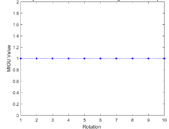
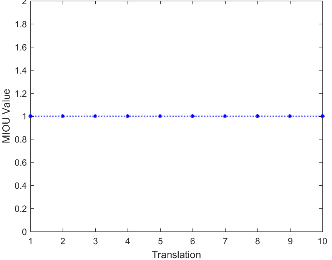
(a) Rotation invariant analysis
(b) Translation invariant analysis
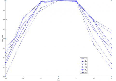
(c) Scala invariant analysis
Figure 8. Geometric invariant analysis on Mortise_and_Tenon_DB
In this experiment, the results show that under limited set transformation conditions, for the 10 models randomly selected from the Mortise_and_Tenon_DB database, the value of the algorithm parameter $\rho$ approaches 1 in the translation and rotation transformation tests, indicating strong geometric invariance of our algorithm. In the scaling transformation tests, due to overlapping of some points within the visual space leading to point loss, the value of the algorithm parameter $\rho$ did not stabilize near 1, indicating weaker geometric invariance of our algorithm. Furthermore, as the compression rate increases, more points are lost during scaling transformations, the spatial structure is disrupted, and the scalability and invariance of the algorithm decrease.
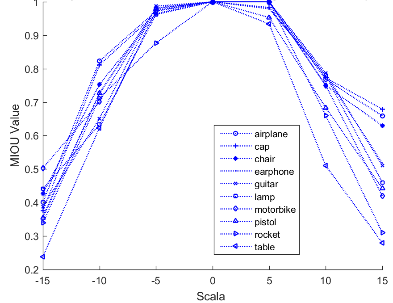
(a) Rotation invariant analysis
(b) Translation invariant analysis
(c) Scala invariant analysis
Figure 9. Geometric invariant analysis on the ShapeNetPart dataset
This paper proposes "Multi-domain adaptive graph convolution algorithm based on visual computing theory and its scene segmentation application". Inspired by the 3D vision of primates, a 3D vision computing theory is proposed; based on this, the algorithm of nearest neighbor space range of graph convolution is definition, and an adaptive graph convolution algorithm based on 3D vision selectivity is proposed. Inspired by the serial/parallel processing model of primate visual information, a single-link/multi-link depth adaptive graph convolution algorithm based on 3D visual selectivity is constructed to learn and integrate the depth and breadth visual features of point clouds. and global and local visual features; the MLP algorithm with shared weights is used to achieve object segmentation. On ShapeNetPart and custom Mortise_and_Tenon_DB, compare with algorithms such as PointNet, PointNet++, KPConv deform, 3D GCN and My algorithm to verify the segmentation performance and geometric invariance of this algorithm. The experimental results show that the algorithm of this paper has good segmentation performance, and the segmentation success rate reaches 90.9%; the algorithm in this paper has strong geometric invariance, rotation and translation transformations have geometric invariance, and in the interval [-0.15,0.15], the telescopic transformation has limited geometric invariance. transsexual.
Future optimizations of the algorithm will focus on two main aspects to improve performance:
(1) Verify the feasibility and advantages of this algorithm on more data sets (especially large scene data sets), and prove the universality of the algorithm.
(2) The multi-link parallel depth vision algorithm involves many parameters, the parameter settings are more complex, and parameter optimization and algorithm problems are prominent. Parameter optimization and adaptive setting are important follow-up research directions.
(3) The algorithm parameter setting determines the computational complexity of the algorithm, and determines the time and space complexity of the algorithm. With the improvement of algorithm optimization methods, the time and space complexity of the algorithm under optimization conditions will be further explored.
This work is supported by The Introduce intellectual resources Projects of Hebei Province of China in 2023 (The depth computing technology of double-link based on visual selectivity, Grant No.:2060801), the Key R&D Projects in Hebei Province of China (Grant No.: 19210111D); The Special project of sustainable development agenda innovation demonstration area of the R&D Projects of Applied Technology in Chengde City of Hebei Province of China (Grant No.: 202205B031, 202205B089, 202305B101). Higher Education Teaching Reform Research Projects of National Ethnic Affairs Commission of the People's Republic of China in 2021 (Grant No.: 21107,21106); Wisdom Lead Innovation Space Projects (Grant No.: HZLC2021004).
[1] Zamanakos, G., Tsochatzidis, L., Amanatiadis, A., Pratikakis, I. (2021). A comprehensive survey of LIDAR-based 3D object detection methods with deep learning for autonomous driving. Computers & Graphics, 99: 153-181. https://doi.org/10.1016/j.cag.2021.07.003
[2] Peters, A., Knoll, A.C. (2024). Robot self-calibration using actuated 3D sensors. Journal of Field Robotics, 41(2): 327-346. https://doi.org/10.1002/rob.22259
[3] Abbasi, R., Bashir, A.K., Alyamani, H. J., Amin, F., Doh, J., Chen, J. (2022). Lidar point cloud compression, processing and learning for autonomous driving. IEEE Transactions on Intelligent Transportation Systems, 24(1): 962-979. https://doi.org/10.1109/TITS.2022.3167957
[4] Mahmood, B., Han, S., Lee, D.E. (2020). BIM-based registration and localization of 3D point clouds of indoor scenes using geometric features for augmented reality. Remote Sensing, 12(14): 2302. https://doi.org/10.3390/rs12142302
[5] Abreu de Souza, M., Alka Cordeiro, D.C., Oliveira, J.D., Oliveira, M.F.A.D., Bonafini, B.L. (2023). 3D multi-modality medical imaging: Combining anatomical and infrared thermal images for 3D reconstruction. Sensors, 23(3): 1610. https://doi.org/10.3390/s23031610
[6] Shi, S., Jiang, L., Deng, J., Wang, Z., Guo, C., Shi, J., Li, H. (2023). PV-RCNN++: Point-voxel feature set abstraction with local vector representation for 3D object detection. International Journal of Computer Vision, 131(2): 531-551. https://doi.org/10.1007/s11263-022-01710-9
[7] Wang, Z., Wei, Y., Rao, Y., Zhou, J., Lu, J. (2023). 3d point-voxel correlation fields for scene flow estimation. IEEE Transactions on Pattern Analysis and Machine Intelligence, 45(11): 13621-13635. https://doi.org/10.1109/TPAMI.2023.3294355
[8] Liu, Z., Tang, H., Lin, Y., Han, S. (2019). Point-voxel CNN for efficient 3D deep learning. Advances in Neural Information Processing Systems, 32, arXiv:1907.03739. https://doi.org/10.48550/arXiv.1907.03739
[9] Rubino, C., Crocco, M., Del Bue, A. (2017). 3D object localisation from multi-view image detections. IEEE Transactions on Pattern Analysis and Machine Intelligence, 40(6): 1281-1294. https://doi.org/10.1109/TPAMI.2017.2701373
[10] Lin, D., Li, Y., Cheng, Y., Prasad, S., Nwe, T.L., Dong, S., Guo, A. (2022). Multi-view 3D object retrieval leveraging the aggregation of view and instance attentive features. Knowledge-Based Systems, 247: 108754. https://doi.org/10.1016/j.knosys.2022.108754
[11] Hong, R., Hu, Z., Wang, R., Wang, M., Tao, D. (2016). Multi-view object retrieval via multi-scale topic models. IEEE Transactions on Image Processing, 25(12): 5814-5827. https://doi.org/10.1109/TIP.2016.2614132
[12] Qi, C.R., Su, H., Mo, K., Guibas, L.J. (2017). Pointnet: Deep learning on point sets for 3d classification and segmentation. In Proceedings of the IEEE Conference on Computer Vision and Pattern Recognition, Honolulu, HI, USA, pp. 652-660. https://doi.org/10.1109/CVPR.2017.16
[13] Qi, C.R., Yi, L., Su, H., Guibas, L.J. (2017). Pointnet++: Deep hierarchical feature learning on point sets in a metric space. Advances in Neural Information Processing Systems, arXiv:1706.02413. https://doi.org/10.48550/arXiv.1706.02413
[14] Özbay, E., Cinar, A.C. (2019). A comparative study of object classification methods using 3D Zernike moment on 3D point clouds. Traitement du Signal, 36(6): 549-555. https://doi.org/10.18280/ts.360610
[15] Nguyen, T.A., Lee, S. (2018). 3D orientation and object classification from partial model point cloud based on pointnet. In 2018 IEEE International Conference on Image Processing, Applications and Systems (IPAS), Sophia Antipolis, France, pp. 192-197. https://doi.org/10.1109/IPAS.2018.8708896
[16] Cao, P., Chen, H., Zhang, Y., Wang, G. (2019). Multi-view frustum pointnet for object detection in autonomous driving. In 2019 IEEE International Conference on Image Processing (ICIP), Taipei, Taiwan, pp. 3896-3899. https://doi.org/10.1109/ICIP.2019.8803572
[17] Zhao, Y.M., Su, G.A., Yang, H., Zhao, T.S., Jin, S.W., Yang, J.N. (2022). Graph convolution algorithm based on visual selectivity and point cloud analysis application. Traitement du Signal, 39(5): 1507-1516. https://doi.org/10.18280/ts.390507
[18] Wang, Y., Geng, G., Zhou, P., Zhang, Q., Li, Z., Feng, R. (2022). GC-MLP: Graph convolution MLP for point cloud analysis. Sensors, 22(23): 9488. https://doi.org/10.3390/s22239488
[19] Fan, H.Y., Zhao, Y.M., Su, G.A., Zhao, T.S., Jin, S.W. (2023). The multi-view deep visual adaptive graph convolution network and its application in point cloud. Traitement du Signal, 40(1): 31-41. https://doi.org/10.18280/ts.400103
[20] Qian, G., Abualshour, A., Li, G., Thabet, A., Ghanem, B. (2021). PU-GCN: Point cloud upsampling using graph convolutional networks. In Proceedings of the IEEE/CVF Conference on Computer Vision and Pattern Recognition, Nashville, TN, USA, pp. 11683-11692. https://doi.org/10.48550/arXiv.1912.03264
[21] Wang, Y., Sun, Y., Liu, Z., Sarma, S.E., Bronstein, M.M., Solomon, J.M. (2019). Dynamic graph CNN for learning on point clouds. ACM Transactions on Graphics, 38(5): 1-12. https://doi.org/10.1145/3326362
[22] Shen, Y., Feng, C., Yang, Y., Tian, D. (2018). Mining point cloud local structures by kernel correlation and graph pooling. In Proceedings of the IEEE Conference on Computer Vision and Pattern Recognition, Salt Lake City, UT, USA, pp. 4548-4557. https://doi.org/10.1109/CVPR.2018.00478
[23] Liu, Y., Fan, B., Xiang, S., Pan, C. (2019). Relation-shape convolutional neural network for point cloud analysis. In Proceedings of the IEEE/CVF Conference on Computer Vision and Pattern Recognition, Long Beach, CA, USA, pp. 8895-8904.
[24] Lin, Z.H., Huang, S.Y., Wang, Y.C.F. (2020). Convolution in the cloud: Learning deformable kernels in 3D graph convolution networks for point cloud analysis. In Proceedings of the IEEE/CVF Conference on Computer Vision and Pattern Recognition, Seattle, WA, USA, pp. 1800-1809. https://doi.org/10.1109/CVPR42600.2020.00187
[25] Zhao, Y., Su, G., Yang, H., Zhao, T., Jin, S., Yang, J. (2022). Graph convolution algorithm based on visual selectivity and point cloud analysis application. Traitement du Signal, 39(5): 1507-1516. https://doi.org/10.18280/ts.390507
[26] Fan, H., Zhao, Y., Su, G., Zhao, T., Jin, S. (2023). The multi-view deep visual adaptive graph convolution network and its application in point cloud. Traitement du Signal, 40(1): 31-41. https://doi.org/10.18280/ts.400103
[27] Guo, M.H., Cai, J.X., Liu, Z.N., Mu, T.J., Martin, R.R., Hu, S.M. (2021). Pct: Point cloud transformer. Computational Visual Media, 7: 187-199. https://doi.org/10.1007/s41095-021-0229-5
[28] Lee, H., Jeon, J., Hong, S., Kim, J., Yoo, J. (2023). TransNet: Transformer-based point cloud sampling network. Sensors, 23(10): 4675. https://doi.org/10.3390/s23104675
[29] Zhao, Y., Yang, H., Su, G. (2021). Design and application of a slow feature algorithm coupling visual selectivity and multiple long short-term memory networks. Traitement du Signal, 38(5): 1521-1530. https://doi.org/10.18280/ts.380529
[30] Fan, H., Zhao, Y., Su, G., Zhao, T., Jin, S. (2023). The multi-view deep visual adaptive graph convolution network and its application in point cloud. Traitement du Signal, 40(1): 31-41. https://doi.org/10.18280/ts.400103
[31] Chang, A.X., Funkhouser, T., Guibas, L., Hanrahan, P., Huang, Q., Li, Z., Yu, F. (2015). Shapenet: An information-rich 3D model repository. arXiv preprint arXiv:1512.03012. https://doi.org/10.48550/arXiv.1512.03012
[32] Klokov, R., Lempitsky, V. (2017). Escape from cells: Deep Kd-networks for the recognition of 3D point cloud models. In Proceedings of the IEEE International Conference on Computer Vision, Venice, Italy, pp. 863-872. https://doi.org/10.1109/ICCV.2017.99
[33] Huang, Q., Wang, W., Neumann, U. (2018). Recurrent slice networks for 3D segmentation of point clouds. In Proceedings of the IEEE Conference on Computer Vision and Pattern Recognition, Salt Lake City, UT, USA, pp. 2626-2635. https://doi.org/10.1109/CVPR.2018.00278
[34] Shen, Y., Feng, C., Yang, Y., Tian, D. (2018). Mining point cloud local structures by kernel correlation and graph pooling. In Proceedings of the IEEE Conference on Computer Vision and Pattern Recognition, Salt Lake City, UT, USA, pp. 4548-4557. https://doi.org/10.1109/CVPR.2018.00478
[35] Li, J., Chen, B.M., Lee, G.H. (2018). So-net: Self-organizing network for point cloud analysis. In Proceedings of the IEEE Conference on Computer Vision and Pattern Recognition, Salt Lake City, UT, USA, pp. 9397-9406. https://doi.org/10.1109/CVPR.2018.00979
[36] Thomas, H., Qi, C.R., Deschaud, J.E., Marcotegui, B., Goulette, F., Guibas, L.J. (2019). Kpconv: Flexible and deformable convolution for point clouds. In Proceedings of the IEEE/CVF International Conference on Computer Vision, Seoul, Korea, pp. 6411-6420. https://doi.org/10.1109/ICCV.2019.00651
[37] Liu, Y., Fan, B., Xiang, S., Pan, C. (2019). Relation-shape convolutional neural network for point cloud analysis. In Proceedings of the IEEE/CVF Conference on Computer Vision and Pattern Recognition, Long Beach, CA, USA, pp. 8895-8904. https://doi.org/10.1109/CVPR.2019.00910