Islam Hassani*![]() | Redha Bendoumia
| Redha Bendoumia![]() | Abderrezak Guessoum
| Abderrezak Guessoum![]() | Ahcene Abed
| Ahcene Abed![]()
© 2024 The authors. This article is published by IIETA and is licensed under the CC BY 4.0 license (http://creativecommons.org/licenses/by/4.0/).
OPEN ACCESS
In communication systems as public switched telephone networks and tele-and-vision-conferencing system, addressing the challenge of sparse acoustic echo is of paramount importance. The sparse impulse response identification is very essential in acoustic echo cancellation systems (AEC) exactly in sparse acoustic environments. This paper introduces an enhanced improved proportionate normalized-least-mean-square (IP-NLMS) algorithm, utilizing efficient variable step-size parameters and adapting only the active coefficients based on selection bloc for reducing the computational complexity. The proposed Variable Selection Coefficients IP-NLMS algorithm (VSC-IP-NLMS) focuses on adapting the selected active coefficients of the sparse impulse response (SIR), in order to both accuracy and convergence speed. Extensive simulations conducted under various sparse environments confirm the efficacy of the proposed algorithm. As important characteristic of this proposed VSC-IP-NLMS, it achieves these remarkable results with significantly reduced computational complexity compared to sparse and variable adaptive filtering algorithms, offering a promising avenue for improving the quality of communication systems.
adaptive filter, IP-NLMS algorithm, sparse impulse responses, communication system, variable step-size
Recently, the rise of telecommunications has facilitated the adoption of digital communication tools, enabling people to make phone calls virtually from any location around the world. However, the conversation is sometimes not clear in non-quiet places, this disturbance is called noise, which generates a weak communication between correspondents. Recently, several research papers have been published based on adaptive filtering algorithms, which have been implemented on several telecommunication fields, such as acoustic echo and noise reduction to accelerate the convergence adaptation and enhancing the quality of conversations [1-3]. Adaptive filtering algorithms are largely used in acoustic echo cancellation [4-6]. Several researches have been conducted to address the identification problem in the time domain and in the frequency domain [7, 8]. We cite for example, the basic Least Mean Square (LMS) and normalized LMS version which are extensively used especially for their simplicity of implementations. Other filtering algorithms have been proposed for AEC applications [9-11]. The problem of echo becomes more complex in situations where the excitation signal is strongly non-stationary and the echo path is variable. To give the solution for all these problems, an echo canceller can be employed, where the Impulse Response (IR) identification is done by using digital Finite IR filter (FIR) [12-14].
Generally, in an adaptive filtering algorithm, the increase in the adaptation step-size, results to very fast convergence speed with important fluctuations around the average trajectory. Recently, several algorithms based on variable step-sizes are proposed to solve the problems mentioned above, using several criteria [15-17]. All these variable step-size adaptive filtering versions can theoretically be used to eliminate the fluctuations but exactly when the echo channel is characterized by a dispersive IR. In some applications, the acoustic environment is characterized by SIR. In this case, the adaptive filtering algorithms presented previously give a poor performance in terms of convergence speed and final steady-state regime. To resolve this problem in sparse environment case, several versions of adaptive filtering algorithms have been developed such as the proportionate NLMS algorithm (PNLMS) [18]. Another algorithm called the IP-NLMS has been also proposed to find the solution with dispersive or sparse environments [19]. These algorithms update a large part of adaptive filter coefficients to reach acceptable performances. Complexity reduction of the adaptive algorithms is an essential solution for the real-time implementation of AEC systems [18-20].
Noting that the non-sparse NLMS algorithm presents a poor performance exactly in acoustical sparse impulse responses system. While the IP-NLMS algorithm performs better in these situations, but it requires a high computational complexity. To resolve these problems, we introduce an improved version called the Variable Selection Coefficients IP-NLMS algorithm (VSC-IP-NLMS). This new algorithm reduces computational complexity by focusing only on active coefficients adaptation for resolving the problem of IP-NLMS. As we propose to use an efficient variable step-sizes to accelerate the convergence rate and minimize the final steady-state error. This new approach balances efficiency performance with very low computational complexity exactly in sparse impulse responses systems.
The remaining parts of this paper are divided into the following sections: in the second section, the description of AEC system adapted by non-proportionate NLMS and improved proportionate algorithms is given; then, the proposed IP-NLMS algorithm is developed in the third section. The fourth section is dedicated to experimental results of the proposed algorithm compared to the sparsity-aware NLMS versions. Finally, a conclusion is done in the last section.
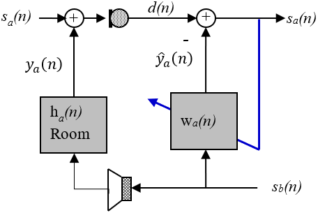
A teleconferencing system consists of two conference rooms in both of which microphones and loudspeakers are installed. The loudspeaker and microphone are related with acoustic channel formed by large reflections at the boundaries of the closed environments. The far-end speech played in the loudspeakers that is captured by the microphone signal is transmitted back to the far-end. The loudspeaker signal (signal of second room $\mathrm{B}, s_b(n)$) in both cases is convoluted by the locale room IR, $h_a(n)$. However, the first signal $s_a(n)$ is filtered by the impulse response $h_b(n)$.
$y_b(n)=s_b(n) * h_a(n)$ (1)
$y_a(n)=s_a(n) * h_b(n)$ (2)
where, $\left({ }^*\right)$ is the convolution operation. The two echo paths $h_a(n)$ and $h_b(n)$ represent the result of the reflection and the attenuation of the sound by the walls and the objects in the two rooms. In any teleconferencing system, it is very important to eliminate the two acoustic echoes $y_a(n)$ and $y_b(n)$ added in the two microphones installed in two rooms using two acoustic echo cancellation systems. In the AEC system, the adaptive filter is employed to identify the room IR. The filter needs to be updated continuously, because the characteristics of the room vary in time with the movement of people and objects [4, 5]. In Figure 1, $s_b(n)$ is convoluted by $\operatorname{IR} h_a(n)$ of room, and then captured, simultaneously, by a microphone with the $s_a(n)$. In other hand, $s_b(n)$ is convoluted by an updating filter $w_a(n)$ that is used to estimate the $\operatorname{IR} h_a(n)$, and subtracted from the output microphone $d(n)$. Noting that, the output signal of $w_a(n)$ represents the acoustic echo estimation.
To update the adaptive filter $w_a(n)$, we use the error signal during silent periods of $s_a(n)$. This error is given by:
$e(n)=d(n)-\hat{y}(n)$ (3)
$d(n)=s_a(n)+s_b(n) * h_a(n)$ (4)
$\hat{y}(n)=s_b(n) * w_a(n)$ (5)
Inserting Eq. (4) and Eq. (5) in Eq. (3), we obtain
$e(n)=s_a(n)+s_b(n) * h_a(n)-s_b(n) * w_a(n)$ (6)
$e(n)=s_a(n)+s_b(n) *\left[h_a(n) * w_a(n)\right]$ (7)
In the steady-state regime, the filter $w_a(n)$ converges to the room IR (i.e., $h_a(n)=w_{a, o p t}(n)$), and the calculated error becomes:
$e(n)=s_a(n)$ (8)
Figure 1. Basic AEC system
2.1 Classical adaptive filtering algorithms
According to Eq. (8), we note that the resulting error $e(n)$ is used to approximate the near-end speaker $s_a(n)$. This result is obtained after convergence of optimal coefficients $w_{a, o p t}(n)$ to the coefficients of the real impulse response $h_a(n)$. The LMS algorithm is the most commonly used due to its simplicity of implementation, its reduced complexity and its numerical stability, but this latter has some drawbacks such as: its poor performances against long and time varying echo paths; its very sensitivity against non-stationarity input signals.
To make the convergence behavior independent of input energy of adaptive filter, the NLMS algorithm derived from the LMS has been proposed. This normalized version is one of the most used adaptive algorithms in AEC applications. The NLMS reduces the MSE values between desired-response signal and filter output [1-3]. Eq. (9) presents the update recursive formula produced by this algorithm:
$\boldsymbol{w}_{\boldsymbol{a}}(n+1)=\boldsymbol{w}_{\boldsymbol{a}}(n)+\frac{\mu \boldsymbol{s}_{\boldsymbol{b}}(n) e(n)}{\boldsymbol{s}_{\boldsymbol{b}}^T(n) \boldsymbol{s}_{\boldsymbol{b}}(n)}$ (9)
A very small parameter $\xi_{\text {nlms }}$ must be added in the denominator to overcome the problem of division by zero when the quantity $\left[\mathbf{s}_{\boldsymbol{b}}^{\mathrm{T}}(n) \mathbf{s}_b(n)\right]$ takes small values or a zero value. Therefore, the finale equation is given by:
$\boldsymbol{w}_{\boldsymbol{a}}(n+1)=\boldsymbol{w}_{\boldsymbol{a}}(n)+\frac{\mu \boldsymbol{s}_{\boldsymbol{b}}(n) e(n)}{\boldsymbol{s}_{\boldsymbol{b}}^{\boldsymbol{T}}(n) \boldsymbol{s}_{\boldsymbol{b}}(n)+\xi_{n l m s}}$ (10)
where, $\mu$ takes its values between 0 and 2 [1-3].
2.2 Sparse adaptive filtering algorithms
Practically in teleconferencing AEC systems, the length of the acoustic IR $h(n)$ can reach 2048 filter taps which is equivalent to a duration of about 256 ms. The acoustic sparse system is characterized by impulse responses that have the great part of its taps are absent or close to zero (i.e. inactive coefficients) and only a few coefficients have large magnitudes (active coefficients) [18-20].
Several sparsity-aware adaptive algorithms have been developed to identify the sparse IR exactly to improve the NLMS algorithm’s poor performances in teleconferencing systems. Duttweiler propose the Proportionate NLMS algorithm [20], in order to increase the initial convergence speed, by giving a large adaptation gain to large coefficients, in the other hand, it provides a minimal gain of adaptation for small coefficients, which results to a poor convergence rate after the initial phase.
It is crucial to highlight that PNLMS algorithm can be deteriorated when the echo path is a dispersive type. Benesty and Gay [19] proposed the IP-NLMS algorithm. This algorithm is a combination between non-proportionate and proportionate NLMS adaptation. The update formula of the IP-NLMS is described by:
$\boldsymbol{w}_{\boldsymbol{a}}(n+1)=\boldsymbol{w}_{\boldsymbol{a}}(n)+\frac{\mu Q(n) \boldsymbol{s}_{\boldsymbol{b}}(n) e(n)}{\boldsymbol{s}_{\boldsymbol{b}}^T(n) Q(n) \boldsymbol{s}_{\boldsymbol{b}}(n)+\xi_{I P}}$ (11)
The diagonal control matrix $Q(n)$ is used to determine exact step-size value of each coefficient. This matrix is defined as follows:
$Q(n)=\left[\begin{array}{cccc}q_1(n) & 0 & \cdots & 0 \\ 0 & q_2(n) & \cdots & 0 \\ \vdots & \vdots & \ddots & \vdots \\ 0 & 0 & \cdots & q_M(n)\end{array}\right]$ (12)
where, $\operatorname{Diag}\{Q(n)\}=\left[q_1(n), q_2(n), \ldots, q_M(n)\right]$ and $M$ is the SIR length. The diagonal elements of $Q(n)$ is denoted by $q_m(n)$ which are estimated as
$q_m(n)=\frac{(1-\alpha)}{2 M}+\frac{(1+\alpha)\left|\boldsymbol{w}_{a, m}(n)\right|}{2\left\|\boldsymbol{w}_a(n)\right\|_1+\varphi}$ (13)
$\left|\mathbf{w}_{a, m}(n)\right|_1$ is defined as the $l_1$-norm
$\left\|\boldsymbol{w}_a(n)\right\|_1=\sum_{i=1}^M \boldsymbol{w}_{a, i}(n)$ (14)
where, $\xi_{I P}=((1-\alpha) / 2 M) \xi_{n l m s}$ and $\alpha$ is a control parameter must be fixed between -1 and 1. Exactly at the initial convergence of adapting filter, we use the small number that introduced to prevent numerator from the division by zero. The IP-NLMS algorithm becomes identical to the basic NLMS when $\alpha=-1$, also, if this scalar equals to 1 , the two algorithms IP-NLMS and P-NLMS become similar. In AEC applications, the suitable choices of $\alpha$ are $\alpha=0,-0.5$ or -0.75 [20].
3.1 Proposition methodology
For a long adaptive filter application in AEC system, the complexity load of IP-NLMS version is very important compared with the basic-NLMS. In long SIR, large inactive coefficients (very small, equal or close to zero) are present, and only a few active coefficients that have large magnitudes. The active coefficients number of adaptive filter for Sparse IR identification is an important parameter.
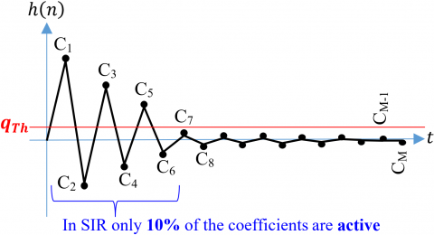
Figure 2. Active coefficient selection procedure
We note that $C_i$ are the coefficients of the sparse impulse response. For example, in Figure 2, the all coefficients greater than a threshold value $q_{T h}$ are considered as active coefficients $\left(C_1, C_2, C_3, C_4\right.$ and $\left.C_5\right)$ and all others coefficients are inactive or not important. It is very important to adapt only the active coefficients to minimize the computational complexity. For this objective, we suggest a modified adaptive filtering NLMS with very low complexity by adapting only the active coefficients by using an active coefficients selection bloc based on averaging constant detection approach.
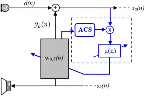
The new AEC system in SIR based on the selection of active coefficients and variable step-sizes parameters with low complexity is illustrated in Figure 3.
Figure 3. AEC system based on proposed algorithm with ACS is active coefficient selection
In new AEC system, we proposed to implement new bloc used to select the active coefficient of adaptive filter. After this step, we proposed to adapt only these active coefficients (presented by new adaptive filter $\mathbf{w}_{a, S}(n)$) to decrease the complexity load. In the proposed structure presented in Figure 3, we propose to adapt only the new active coefficients vector combined with the new variable step-sizes parameters that are updated recursively. The new adaptation formula is written as:
$\begin{gathered}\boldsymbol{w}_{a, S}(n+1)= \\ \boldsymbol{w}_{\boldsymbol{a}, S}(n)+\frac{\mu_s(n) Q_S(n) \boldsymbol{s}_{b, S}(n) e(n)}{\boldsymbol{s}_{b, S}^T(n) Q_S(n) \boldsymbol{s}_{b, S}(n)+\xi_{I P, S}}\end{gathered}$ (15)
where, $\boldsymbol{w}_{\boldsymbol{a}, S}(n)$ represents the new vector contains only active coefficients of original adaptive filter without the small and inactive coefficients one.
3.2 Diagonal control matrix $Q_s(n)$
In this proposed version, we use new diagonal control matrix $Q_S(n)$ that is introduced to determine and adapt only the active filter coefficients. This matrix is written as:
$Q_S(n)=\left[\begin{array}{cccc}q_{S, 1}(n) & 0 & \cdots & 0 \\ 0 & q_{S, 2}(n) & \cdots & 0 \\ \vdots & \vdots & \ddots & \vdots \\ 0 & 0 & \cdots & q_{S, M}(n)\end{array}\right]$ (16)
where, $\operatorname{diag}\left\{Q_S(n)\right\}=\left[q_{s, 1}(n), q_{S, 2}(n), \ldots, q_{S, M}(n)\right]$. The modified diagonal coefficients of $Q_S(n)$ is denoted by $q_{S, j}(n)$ with $0 \leq j \leq M-1$ which are estimated as:
$q_{S, j}(n)=\frac{(1-\alpha)}{2 M}+\frac{(1+\alpha)\left|\boldsymbol{w}_{a, S, j}(n)\right|}{2\left\|\boldsymbol{w}_{a, S}(n)\right\|_1+\varphi}$ (17)
To select exactly the active coefficients of $\boldsymbol{w}_{a, S}(n)$, we propose as a first step to calculate the threshold using the mean value of the matrix diagonal elements that is given by:
$q_{T h}=\gamma \sum_{j=1}^M q_{S, j}(n)$ (18)
As a second step, we find the $S$ active filter coefficients by omparing each element of step-size control matrix with the alculated threshold value.
$\left\{\begin{array}{l}\text { if } q_j(n) \geq q_{T h} \rightarrow w_j(n) \text { is an active coefficient } \\ \text { if } q_j(n)<q_{T h} \rightarrow w_j(n) \text { is an inactive coefficient }\end{array}\right.$
$\left\{\begin{array}{l}\text { Active coefficient } \rightarrow w_j(n) \text { is adapt in Algorithm } \\ \text { Inactive coefficient } \rightarrow w_j(n) \text { is non }- \text { adapt }\end{array}\right.$
Finally, we extract all $j$ positions of active coefficients that is used to identify the new vector of active coefficients of Sparse IR. This latter apply that we adapt only efficient S coefficients, and $\xi_{I P, S}$ is a scalar regularization parameter defined as, $\xi_{I P, S}=((1-\alpha) / 2 S) \xi_{n l m s}$. The detailed steps of active coefficients selection are presented in Figure 4.
Figure 4. Detailed steps of active coefficients selection with variable step-size parameter
3.3 Optimal step-size estimation
Employing variable step-sizes is a crucial technique that enhances convergence and adaptability. Instead of using a fixed step-size, which may lead to slow progress or overshooting, variable step-sizes allow the algorithm to adjust its steps dynamically. By decreasing the step-size in regions where the function is in decreasing and increasing it in flatter areas, the algorithm can efficiently navigate complex, irregular, or non-conditioned optimization problems. The role of the weight-error vectors $\boldsymbol{\epsilon}(n)$ becomes apparent in the adaptation process, where they serve as a means to quantify the disparity between the desired optimum tap-weight vector $\boldsymbol{h}_a(n)$ and the estimated coefficients filter $\boldsymbol{w}_{\boldsymbol{a}, \boldsymbol{S}}(n)$.
$\boldsymbol{\epsilon}(n)=\boldsymbol{h}_a(n)-\boldsymbol{w}_{a, S}(n)$ (19)
The mean-square deviation (MSD) quantifies the average squared disparity between the desired and actual weight-error vectors, thereby providing a measure of how closely the adaptive filters approximate the desired impulse response. A lower MSD signifies a higher degree of accuracy and, consequently, better overall performance. The equation for calculating the MSD is as follows:
$c(n)=E\left[\|\boldsymbol{\epsilon}(n)\|^2\right]=E\left\lceil\left\|\boldsymbol{h}_a(n)-\boldsymbol{w}_{a, S}(n)\right\|^2\right\rceil$ (20)
After substituting Eq. (20) into basic-NLMS Eq. (10) and performing the necessary calculations to determine the squared Euclidean model:
$\begin{gathered}c(n)-c(n-1)=\mu_1^2 E\left[\frac{e(n)^2}{s_{b, s}^T(n) s_{b, s}(n)+\xi_{n l m s}}\right] \\ -2 \mu_1 E\left[\frac{\epsilon^T(n-1) s_{b, s}(n) e(n)}{s_{b, s}^T(n) s_{b, s}(n)+\xi_{n l m s}}\right]\end{gathered}$ (21)
By observing that $c(n)-c(n-1)=f(\mu)$, selecting an optimal value of $\mu$ that maximizes the function $f(\mu)$ guarantees the most substantial reduction in the mean-square deviation (MSD) from one iteration ( $n-1)$ to the next $(n)$, resulting in $c(n)$ being less than $c(n-1)$. In simpler terms, this means that by choosing the right step-size, we can significantly enhance the algorithm's performance in minimizing the error between the desired output and the actual output at each iteration. This, in turn, leads to a more efficient adaptation process. Considering $c(n)<c(n-1)$, it follows that $f(\mu)$ is less than zero, allowing us to express the relationship as follows:
$\begin{gathered}\mu^2 E\left[\frac{e(n)^2}{s_{b, s}^T(n) s_{b, s}(n)+\xi_{n l m s}}\right] \\ -2 \mu E\left[\frac{\epsilon^T(n-1) s_{b, s}(n) e(n)}{s_{b, S}^T(n) s_{b, S}(n)+\xi_{n l m s}}\right]<0\end{gathered}$ (22)
Based on Eq. (22), the optimal step-size parameter is given by:
$\mu_{o p t}<2\left\{\frac{E\left[\frac{\epsilon^T(n-1) s_{b, S}(n) e(n)}{\left.s_{b, s}^T(n) s_{b, S}(n)+\xi_{n l m s}\right]}\right]}{E\left[\frac{e(n)^2}{s_{b, S}^T(n) s_{b, S}(n)+\xi_{n l m s}}\right]}\right\}$ (23)
We note that
$\mu_{o p t}<2 \vartheta(n)$ (24)
Using the NLMS algorithm and referring to Eq. (25), the optimal step-size value is constrained within the range of $0<$ $\mu_{o p t}<2$. This constraint is dependent on the small parameter $\vartheta(n)$, which is provided as a variable:
$\vartheta(n)<1$ (25)
In the following section, we introduce our innovative approach to parameterize $\mu(n)$ through recursive estimations. This novel adaptation enables us to derive recursive formulas for $\mu_{o p t}$. In the optimal situation, the input signal, denoted as $\mathbf{s}_{b, S}(n)$, for the adaptive filter $\boldsymbol{w}_{\boldsymbol{a}, S}(n)$, and the estimated output error $e(n)$, tend to become decorrelated signals. However, the small parameter $\vartheta(n)$ can be estimated by examining the cross-correlation function between the input signal $\mathbf{s}_{b, S}(n)$ and the output error $e(n)$. We now propose an alternative method for estimating this small quantity $\vartheta(n)$ using a newly derived quantity, $\tilde{\vartheta}(n)$, which is based on minimizing the cross-correlation between $e(n)$ and $\mathbf{s}_{b, S}(n)$.
$\tilde{\vartheta}(n)=\frac{\|\boldsymbol{G}(n)\|^2}{c+\|\boldsymbol{G}(n)\|^2}$ (26)
with $0<c$ and $\left\{c+\|\mathbf{G}(n)\|^2\right\}>\|\mathbf{G}(n)\|^2$. applies that $\tilde{\vartheta}(n)<1$. We note also that the proposed estimation of optimal step-size parameter is presented as
$\mu_{o p t}<2 \times \tilde{\vartheta}(n)$ (27)
We substitute the value of 2 with $\mu_{\max }$, a selection has a purpose for achieving the fastest convergence rate while observing to the condition $\mu_{\max }<2$. Our proposition involves the recursive estimation of the optimal variable step-size parameter, which can be computed as:
$\tilde{\mu}_{o p t}(n)=\mu_{\max } \times \frac{\|\boldsymbol{G}(n)\|^2}{c+\|\boldsymbol{G}(n)\|^2}$ (28)
The vector $\boldsymbol{G}(n)$ is estimated through the minimization of a cross-correlation function between the input signal $\mathbf{s}_{b, S}(n)$ and the output error signal $e(n)$. The estimation of this vector is expressed as follows:
$\boldsymbol{G}(n)=k \boldsymbol{G}(n-1)+(1-k) \frac{s_{b, S}^T(n) e(n)}{s_{b, S}^T(n) s_{b, S}(n)+\varepsilon}$ (29)
with $0<k<1$. The final variable step-size parameter used in updating equation is controlled and adapted using the next condition to guarantee the convergence of adaptive filters,
$\mu(n)= \begin{cases}\mu_{\min } & \text { if } \tilde{\mu}_{o p t}(d)<\mu_{\min } \\ \tilde{\mu}_{o p t}(d) & \text { otherwise }\end{cases}$ (30)
$\mu_{\min }$ represents the potential minimum value necessary to ensure the highest level of quality.
4.1 Signals and parameters of simulation environment
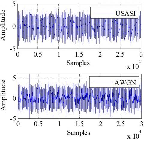
The simulation involves comparing the performance of the Proposed algorithm with three other algorithms: the Basic-NLMS (fixed-and-non-proportionate step-size), the IP-NLMS [19] (fixed-and-proportionate step-size) and the VSS-NLMS [21] (variable-and-nonproportionate step-size). These algorithms are implemented and tested in the MATlab environment. Two types of input signals are used for testing the performances of these algorithms: USASI-noise (USA Standards Institute) and Additive White Gaussian Noise (AWGN). The statistical characteristics of USASI-noise are: a spectrum close to the average spectrum of the speech signal, a spectral range of $32 d B$ and a power of $\sigma_x^2=0.33$. These signals represent the background noise that the AEC system needs to cancel it (see Figure 5). We note that the sparse impulse responses are used to model the characteristics of real rooms. These responses are crucial for simulating the acoustic environment accurately.
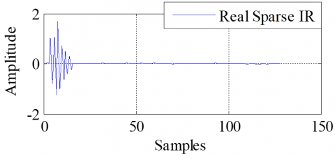
The sparse impulse response is designed with a specific number of active coefficients representing $10 \%$ of the impulse response length. This indicates that only a part of the impulse response is active, which is a common scenario in realacoustic room environments, see Figure 6.
Figure 5. Time evolution of USASI signal and AWGN
Figure 6. SIR, M = 128 with 12 active coefficients
Table 1. Numerical values of simulated adaptive algorithms
|
Algorithms |
Parameters |
|
Basic-NLMS |
$\mu=0.9, \xi_{\text {nlms }}=10^{-6}$ |
|
IP-NLMS |
$\mu=0.9, \xi_{I P}=((1-\alpha) / 2 M) \xi_{n l m s}, \alpha=-0.5$, $\varphi=10^{-6}$ |
|
VSS-NLMS |
$\begin{gathered}\mu_{\max }=0.9, \mu_{\min }=0.02, c=0.00009, k=0.999, \\ \xi_{\text {VSS }}=10^{-6}\end{gathered}$ |
|
Proposed VSC-IP-NLMS |
$\begin{gathered}\mu_{\max }=0.9, \mu_{\min }=0.02, c=0.00009, k=0.999, \\ \xi_{I P, S}=\xi_{I P}, \alpha=-0.5, \varphi=10^{-6}\end{gathered}$ |
The input signals are sampled at 8 kHz, which is the suitable sampling frequency for the applications of speech communication. The simulation is performed over 60 000 iterations, which implies that the algorithms are tested for various scenarios to assess their convergence and performance.
The input Signal-to-Noise Ratio (SNR) is fixed at a high value of 90 dB, indicating that the input signals have a minimal amount of noise compared to the desired signal. Numerical values of the parameters are presented in Table 1.
As criteria of evaluation, we have used subjective and objective criteria. Three subjective measures are used to evaluate the performance of the proposed algorithm: (i) time evolution of the error signals, (ii) the obtained adaptive filters and (iii) the evolution of variable step-size parameters. These measures help assess how well the AEC system cancels the echo and adapts time varying changes. A deep analysis can be also done using the objective criteria, such as: (i) Mean Square Error (MSE) and (ii) Echo Return Loss Enhancement (ERLE). These metrics provide quantifiable measures of how well the AEC system reduces echo and enhances the quality of the desired signals.
The objective evaluation criterion MSE is defined by the following formula:
$M S E_{d B}=10 \log _{10}\left(E\left\|e(n)^2\right\|\right)$ (31)
The other objective evaluation criterion ERLE measures the amount of attenuated echo signal in AEC applications, that is expressed by:
$E R L E_{d B}=10 \log _{10}\left(\frac{E\left\|d(n)^2\right\|}{E\left\|e(n)^2\right\|}\right)$ (32)
4.2 Subjective criteria results
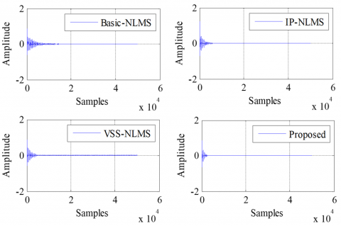
In this subsection, we present the time evolution of all error signals $e(n)$ obtained by the proposed algorithm compared with the desired signal, when using the AWGN signal as input signal. Figure 7 shows the signals of the output error obtained by the four algorithms.
Figure 7. Temporal evolution of error signals
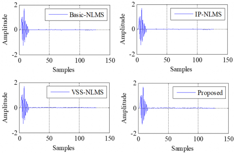
Figure 8. Estimated sparse filters
Figure 8 displays a comparison between the actual coefficients of the sparse filter obtained by four algorithms. The simulations conducted in these figures are performed using the parameter values of Table 1.
Figure 7 presents the signals of the output error obtained by the four different algorithms. These algorithms are used to estimate and adapt to a desired signal with an input signal corrupted by AWGN. The objective is to reach to error signals close to zero, indicating that the algorithms are effectively minimizing the difference between the estimated and desired signals. This figure likely shows how the proposed VSC-IP-NLMS algorithm outperforms the three other algorithms in terms of error signal convergence.
The proposed VSC-IP-NLMS algorithm, show the fastest convergence, that means it reaches a small error signal quickly. We can say that the proposed algorithm is highly efficient for adapting the noisy input signal and approximating the desired signal accurately. The comparison between these error signals helps assess the algorithms performance in terms of signal estimation.
The goal of Figure 8 is examining how well these adaptive filters can approximate the true sparse filter coefficients to the change of input conditions. The Figure 8 demonstrates that proposed and all presented algorithms are estimating the sparse filter coefficients.
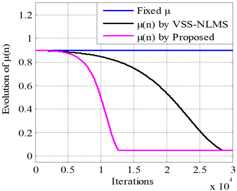
In Figure 9, we illustrate the changes in a particular variable step-sizes parameter achieved by the proposed VSC-IP-NLMS algorithm.
Figure 9. Variable step-size evolution
In Figure 9, the variable step-size values achieved by the proposed VSC-IP-NLMS algorithm are compared with those obtained by the VSS-NLMS algorithm and the Basic fixed-step-size NLMS. The results provide insights into how effectively the proposed algorithm adjusts its step-size during the simulation. A key observation to make here is that the proposed VSC-IP-NLMS algorithm is expected to exhibit the most minimizing and efficient adaptation of step-sizes, which means that it rapidly reduces the step-size when the error signal is close to the steady-state regime, which contributes to faster convergence and minimizes the risk of divergence.
4.3 Convergence rate by MSE criteria
In this section, the primary focus centers on evaluating the convergence speed performance of all algorithms within the context of sparse impulse response identification. The assessment of convergence speed is quantified through the evolution of MSE values, where low MSE values corresponds to high accuracy, indicating a small difference between estimated and desired signals. In the other hand, high MSE values corresponds to large errors and, consequently, less effective algorithm performance.
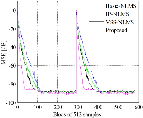
Figure 10. Convergence speed with USASI noise, for M = 128 and Ms = 12
Figure 11. Convergence speed with USASI noise, for M = 256 and Ms = 25
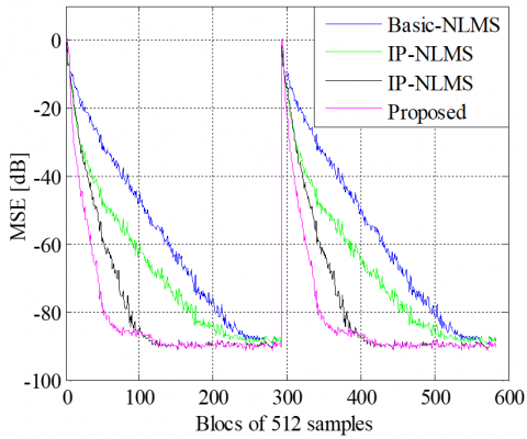
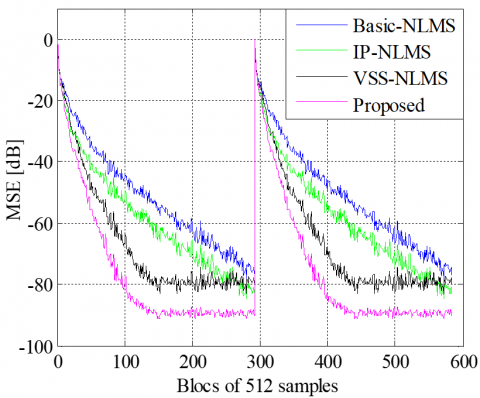
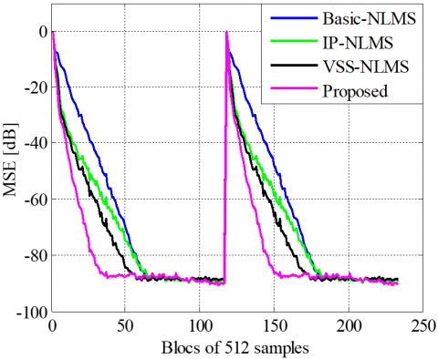
Figure 12. Convergence speed with USASI noise, for M = 512 and Ms = 51
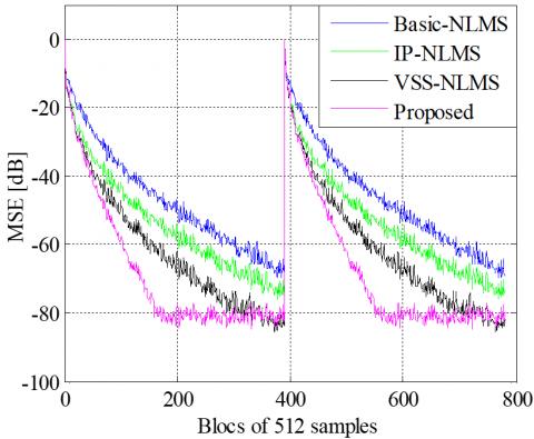
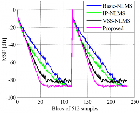
Figure 13. Convergence speed with USASI noise, for M = 1024 and Ms = 102
The measure of tracking capability is derived from an analysis of how rapidly the adaptive filter can adapt to new noise conditions and changes in the impulse response. In this context, it is worth noting that tracking capability performance is a vital aspect of this research.
Figures 10-13 serve as visual representations of the evolution of the MSE when the algorithms are simulated with USASI noise. The input SNR is fixed at a constant value of 90 dB. Experiments are performed under four different sparse acoustic systems, each with different lengths of M, specifically 128, 256, 512, and 1024. The input SNR conditions are maintained at the consistent level of 90 dB.
From Figures 10-13, we can conclude that: (i) Basic-NLMS exhibits a relatively slower convergence rate than IP-NLMS. Its MSE values are higher, indicating that it is less effective for sparse impulse response identification and the tracking capability. (ii) IP-NLMS shows remarkable convergence speed. Its MSE values decrease rapidly and efficiently tracks and estimates desired signals. (iii) The behavior of the VSS-NLMS algorithm is better than Basic-NLMS and IP-NLMS in terms of convergence speed and MSE values. But we note that the final MSE values obtained by this algorithm are high. (vi) The proposed algorithm consistently outperforms all others. It exhibits the fastest convergence and the lowest MSE values, indicating their exceptional ability to track and accurately estimate desired signals, it can be considered as a best candidate in sparse systems.
Figures 14-17 provide experimental results of how the proposed algorithm behaves when operating in the presence of a challenging noise environment, specifically AWGN, with a steady Signal-to-Noise Ratio (SNR) of 90 dB, with different degrees of sparsity.
Figure 14. Convergence speed with AWGN signal, for M = 128 and Ms = 12
Figure 15. Convergence speed with AWGN signal, for M = 256 and Ms = 25
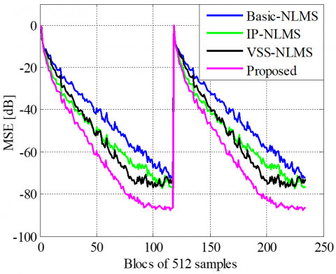
Figure 16. Convergence speed with AWGN signal, for M = 512 and Ms = 51
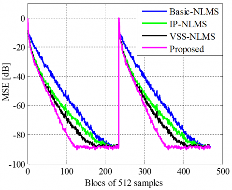
Figure 17. Convergence speed with AWGN signal, for M = 1024 and Ms = 102
Based on these figures, the IP-NLMS algorithm shows a rapid convergence rate and consistently achieves low Mean Square Error (MSE) values compared with Basic-NLMS which presents a slower convergence rate and higher MSE values. As we note that the VSS version gives a fast convergence compared to Basic-NLMS and high MSE values compared to IP-NLMS algorithm. All Figures prove the consistent superiority of the proposed algorithm. It shows a fast convergence with the lowest MSE in AWGN conditions.
All MSE figures confirm that the proposed algorithm has the best performance in USASI and AWGN noise scenarios and with time varying SIR. In terms of statistical analysis, the proposed algorithm converges faster than the other algorithms to the power of the input noise. Its capacity to estimate desired signals and to adapt the changes of noise conditions, gives it a priority to be selected as the best candidates for achieving high-quality noise reduction in real-world speech applications. The superiority of this algorithm is obtained from its selective adaptation of active coefficients. This approach offers a distinct advantage in real-world applications. The adaptation of the proposed algorithm is focused exclusively on the active coefficients, which results to a reduced complexity.
4.4 Echo Return Loss Enhancement criteria
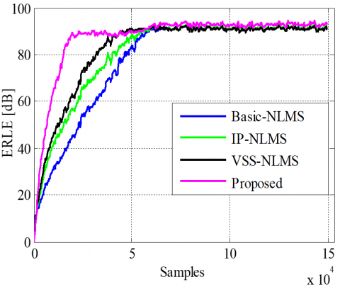
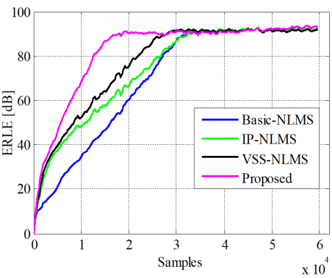
Now, we evaluate the performance of proposed VSC-NLMS and presented algorithms using the ERLE (Echo Return Loss Enhancement) criterion. The ERLE is a critical measure, reflecting the algorithm ability to enhance the quality of acoustic signals by reducing the presence of unwanted echoes. A high ERLE values indicate a more effective algorithm in minimizing echo interference, while low ERLE values signify a poor performance. Figures 18-21 present the evolution of the ERLE when the algorithms are subjected to the input signal of USASI noise. The input SNR is set to 90 dB for all the following evaluations.
Figure 18. ERLE evaluation with USASI noise, for M = 128 and Ms = 12
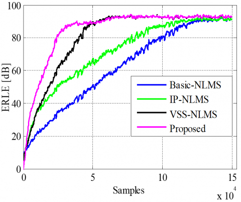
Figure 19. ERLE evaluation with USASI noise, for M = 256 and Ms = 25
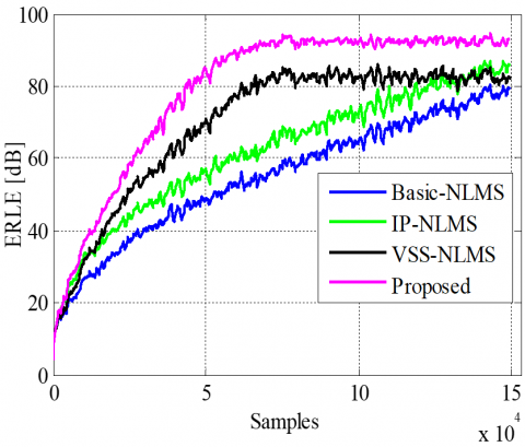
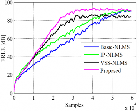
Figure 20. ERLE evaluation with USASI noise, for M = 512 and Ms = 51
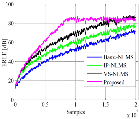
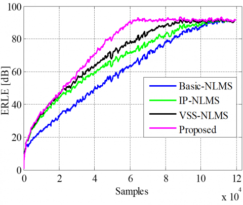
Figure 21. ERLE evaluation with USASI noise, for M = 1024 and Ms = 102
Figure 22. ERLE evaluation with AWGN signal, for M = 128 and Ms = 12
Figure 23. ERLE evaluation with AWGN signal, for M = 256 and Ms = 25
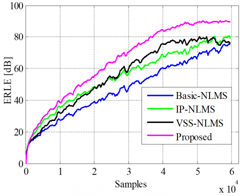
Figure 24. ERLE evaluation with AWGN signal, for M = 512 and Ms = 51
Figure 25. ERLE evaluation with AWGN signal, for M = 1024 and Ms = 102
Figures 18-21 offer a comprehensive analysis of the algorithm performance with respect to the ERLE criterion for two different input signals, the results consistently maintain a high input SNR of 90 dB. After careful examination of all presented ERLE results, it becomes evident that the proposed algorithm outperforms the other algorithms in terms of ERLE enhancement. With an input signal of USASI noise, the proposed algorithm shows high ERLE values for different impulse response lengths, of 128, 256, 512, and 1024.
The ERLE values results obtained in case of AWGN signal are presented in Figures 22-25 for filters lengths, 128, 256, 512 and 1024, respectively. These visual representations offer a comprehensive view of the algorithm performance under different conditions, focusing on their effectiveness in reducing echo interference and enhancing acoustic signal quality. Nothing that we have used the same parameters values presented previously in Table 1.
In the presence of AWGN noise, the proposed algorithm gives superior ERLE values compared to the other algorithms. This show that the proposed algorithm is robust in reducing echo interference under real-world noise scenarios. These findings strongly indicate that the proposed algorithm presents the best solution for enhancing ERLE. The ability of the proposed algorithm to outperform the state of art algorithms in reducing echo interference and improving acoustic signal quality results.
The superior ERLE performance of the proposed algorithm can be attributed to two key characteristics embedded within its design. (i) First, it employs the strategy of minimizing variable step-sizes. This strategic choice allows the algorithm to dynamically adjust its learning rate, ensuring that it converges to the optimum while maintaining stability. By minimizing step-sizes, the algorithm can tune its adaptation process, effectively reducing echo interference and enhancing acoustic signal quality. (ii) Secondly, the algorithm demonstrates its effective performances by adapting only the active coefficient after an adaptive selection process. This means that it focuses its adaptation efforts on the most relevant and impactful coefficients, rather than expending time on irrelevant or less influential ones. By prioritizing active coefficients, the algorithm optimizes its echo reduction capabilities, further contributing to its remarkable ERLE.
4.5 Proposed algorithm performance
In this section, we present the performance of proposed algorithm in term of convergence rate, steady-state error and computational complexity. In Table 2, we present the convergence rate and final MSE values presented previously in section 4.2 exactly for M = 512 and Ms = 51.
Table 2. Performance of proposed algorithm in term of convergence rate and final MSE values
|
Performance |
Algorithms |
USASI |
AWGN |
|
Convergence rate [Bloc] |
Basic- NLMS |
290 |
118 |
|
IP-NLMS |
270 |
110 |
|
|
VSS- NLMS |
150 |
100 |
|
|
Proposed |
140 |
96 |
|
|
Final MSE values [dB] |
Basic- NLMS |
-75 |
-70 |
|
IP-NLMS |
-80 |
-75 |
|
|
VSS- NLMS |
-80 |
-75 |
|
|
Proposed |
-89 |
-86 |
Based on Table 2, we note that the IP-NLMS algorithm and VSS version demonstrate rapid convergence and consistently low Mean Square Error (MSE) values compared to Basic-NLMS, which exhibits slower convergence and higher MSE values. As we can observe the superiority of the proposed algorithm, very fast convergence rate with the lowest MSE values for two situations, USASI and AWGN signals.
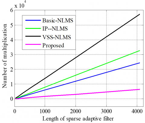
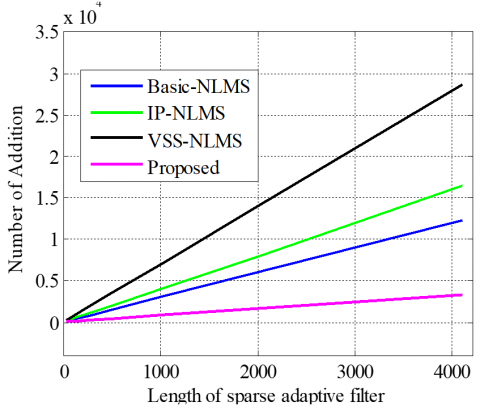
We thoroughly examine the complexities of Basic-NLMS, IP-NLMS, and VSS-NLMS algorithms in comparison to our proposed VSC-IP-NLMS algorithm. We gauge complexity by analyzing the number of multiplications and additions required for each weight update process. Our comparative simulations encompass various sparse impulse responses with different coefficient counts (M = 32, 64, 128, 256, 512, 1024, and 2048). Our proposed algorithm offers a distinct advantage in computational efficiency by exclusively adapting the active coefficients, which constitute only 10% of the total coefficients in sparse impulse responses. This advantage is clearly evident as we adapt only these 10% active coefficients. The theoretical complexity analysis of the four algorithms is summarized in Table 3. Figures 26 and 27 showcase the computational complexity (multiplication and addition operations) across simulations with varying coefficient counts.
Table 3. Theoretical computational complexities, in function of real filter length M and selected active coefficients Ms with Mp: Multiplication and Ad: Addition
|
Algorithms |
Mp |
Ad |
|
NLMS |
6M+4 |
3M+3 |
|
IP-NLMS |
8M+2 |
4M+3 |
|
VSS-NLMS |
14M+8 |
7M+4 |
|
Proposed |
16MS+8 |
8MS+4 |
Figure 26. Computational complexities of all algorithms in terms of multiplication
Figure 27. Computational complexities representation of all algorithms in terms of addition
Based on Table 3, Figure 26, and Figure 27, firstly, as both the filter length (M) and the number of active coefficients (Ms) increase, there's a noticeable uptick in computational cost, suggesting a linear relationship with multiplications and additions. Secondly, among NLMS, IP-NLMS, and VSS-NLMS algorithms, basic NLMS consistently exhibits the lowest computational complexities for M, demanding the fewest multiplications and additions. IP-NLMS follows with higher complexities but offers improved convergence. VSS-NLMS, though the most complex, provides enhanced performance features. Finally, our proposed algorithm emerges with the lowest computational complexities, demonstrating superior efficiency. For instance, at M = 2048 with selected coefficients of Ms = 204, it requires 3,272 multiplications and 1,640 additions, reinforcing its computational advantage over alternatives.
In this paper, we have addressed the critical issue of sparse acoustic impulse response identification, by introducing the Variable Selection Coefficients IP-NLMS algorithm. This proposed algorithm, equipped with efficient variable step-size parameters, focuses on adapting only the active coefficients of the Sparse Impulse Response (SIR). The extensive simulations conducted under various sparse acoustic environments confirm its exceptional efficacy in convergence rate and improving signal quality. The performance evaluation of the proposed algorithm shows the superiority of this latter compared with the state of art algorithms. In the presence of both USASI noise and AWGN signal, it exhibits fast convergence by maintaining the lowest MSE values and best ERLE level for different SIRs. The combination of minimized variable step-sizes and the focus on relevant coefficients results to a powerful, efficient, and robust algorithm. We know that the adaptive algorithms for system identification have significant potential for real-world implementation in various applications for example enhancing the speech quality in case of echo cancellation. However, there are several challenges and limitations that need to be considered for practical implementation, such as: computational complexity, convergence speed, nonlinear distortions and impulse response variability. As a final conclusion, the proposed VSC-IP-NLMS algorithm proposed in this paper offers a promising solution for addressing sparse acoustic impulse response identification. Its exceptional performance, adaptability, and efficiency make it a valuable contribution to the field of acoustic echo cancellation, noise reduction and various real-world applications.
|
AEC |
Acoustic echo cancellation |
|
IP-NLMS |
Improved proportionate NLMS |
|
VSC-IP-NLMS |
Variable Selection Coefficient IP-NLMS |
|
SIR |
Sparse impulse response |
|
LMS |
Least mean square |
|
IR |
Impulse response |
|
FIR |
Finite impulse response |
|
NLMS |
Normalized LMS |
|
PNLMS |
Proportionate NLMS |
|
ACS |
Active coefficient selection |
|
MSD |
Mean-square deviation |
|
USASI |
USA standards institute noise |
|
AWGN |
Additive white gaussian noise |
|
dB |
Decibel |
|
VSS-NLMS |
Variable step-size NLMS |
|
ERLE |
Echo return loss enhancement |
|
MSE |
Mean square error |
|
SNR |
Signal-to-noise ratio |
|
Greek symbols |
|
|
µ |
Fixed step-size |
|
µ(n) |
Variable step-size |
|
µmax |
Maximal step-size value |
|
µmin |
Minimal step-size value |
|
$\alpha$ and $\varphi$ |
Control parameters of sparse adaptation |
|
$c$ and $k$ |
Control parameters of VSS adaptation |
|
$\xi_{n l m s}$, $\xi_{I P}, \xi_{I P, S}$ and $\xi_{V S S}$ |
Very small constants used to avoid division by zero |
|
$\boldsymbol{\epsilon}(n)$ |
Weight-error vectors |
|
Subscripts |
|
|
M |
Length of real sparse impulse response |
|
Ms |
Number of selected active coefficients |
[1] Ramdane, M.A., Benallal, A., Maamoun, M., Hassani, I. (2022). Partial update simplified fast transversal filter algorithms for acoustic echo cancellation. Traitement du Signal, 39(1): 11-19. https://doi.org/10.18280/ts.390102
[2] Bendoumia, R., Kerkar, M., Bouzekkar, S.A. (2019). Acoustic noise reduction by new sub-band forward symmetric adaptive decorrelation algorithms. Applied Acoustic, 152: 118-126. https://doi.org/10.1016/j.apacoust.2019.03.030
[3] Sandoval-Ibarra, Y., Diaz-Ramirez, V.H., Kober, V.I., Karnaukhov, V.N. (2016). Speech enhancement with adaptive spectral estimators. Journal of Communications Technology and Electronics, 61: 672-678. https://doi.org/10.1134/S1064226916060218
[4] Saleem, N., Khattak, M.I., Perez, E.V. (2019). Spectral phase estimation based on deep neural networks for single channel speech enhancement. Journal of Communications Technology and Electronics, 64: 1372-1382. https://doi.org/10.1134/S1064226919120155
[5] Hamidia, M., Amrouche, A. (2016). Improved variable step-size NLMS adaptive filtering algorithm for acoustic echo cancellation. Digital Signal Processing, 49: 44-55. https://doi.org/10.1016/j.dsp.2015.10.015
[6] Hassani, I., Arezki, M., Benallal, A. (2020). A novel set membership fast NLMS algorithm for acoustic echo cancellation. Applied Acoustics, 163: 107210. https://doi.org/10.1016/j.apacoust.2020.107210
[7] Jayakumar, E.P., Sathidevi, P.S. (2018). An integrated acoustic echo and noise cancellation system using cross-band adaptive filters and wavelet thresholding of multitaper spectrum. Applied Acoustics, 141: 9-18. https://doi.org/10.1016/j.apacoust.2018.05.029
[8] Chen, K., Xu, P.Y., Lu, J., Xu, B.L. (2009). An improved post-filter of acoustic echo canceller based on subband implementation. Applied Acoustics, 70(6): 886-893. https://doi.org/10.1016/j.apacoust.2008.10.004
[9] Hamidia, M., Amrouche, A. (2023). A new fast double-talk detector based on the error variance for acoustic echo cancellation. Traitement du Signal, 40(2): 701-707. https://doi.org/10.18280/ts.400229
[10] Samuyelu, B., Kumar, P.R. (2019). Robust normalized subband adaptive filter for acoustic noise and echo cancellation systems. Advances in Modelling and Analysis B, 62(2-4): 61-71. https://doi.org/10.18280/ama_b.622-405
[11] Siva Priyanka, S., Kishore Kumar, T. (2021). Signed convex combination of fast convergence algorithm to generalized sidelobe canceller beamformer for multi-channel speech enhancement. Traitement du Signal, 38(3): 785-795. https://doi.org/10.18280/ts.380325
[12] Lindstrom, F., Schuldt, C., Claesson, I. (2007). An improvement of the two-path algorithm transfer logic for acoustic echo cancellation. IEEE Transactions on Audio, Speech, and Language Processing, 15(4): 1320-1326. https://doi.org/10.1109/TASL.2007.894519
[13] Abadi, M.S.E., Moradiani, F. (2013). A unified approach to tracking performance analysis of the selective partial update adaptive filter algorithms in nonstationary environment. Digital Signal Processing, 23(3): 817-830. https://doi.org/10.1016/j.dsp.2012.12.012
[14] Hassani, I., Benallal, A., Bendoumia, R. (2022). Double-talk robust fast converging and low complexity algorithm for acoustic echo cancellation in teleconferencing system. In Artificial Intelligence and Heuristics for Smart Energy Efficiency in Smart Cities: Case Study: Tipasa, Algeria, pp. 409-420. https://doi.org/10.1007/978-3-030-92038-8_41
[15] Mayyas, K. (2005). Performance analysis of the deficient length LMS adaptive algorithm. IEEE Transactions on Signal Processing, 53(8): 2727-2734. https://doi.org/10.1109/TSP.2005.850347
[16] Bendoumia, R. (2019). Two-channel forward NLMS algorithm combined with simple variable step-sizes for speech quality enhancement. Analog Integrated Circuits and Signal Processing, 98: 27-40. https://doi.org/10.1007/s10470-018-1269-3
[17] Pauline, S.H., Samiappan, D., Kumar, R., Anand, A., Kar, A. (2020). Variable tap-length non-parametric variable step-size NLMS adaptive filtering algorithm for acoustic echo cancellation. Applied Acoustics, 159: 107074. https://doi.org/10.1016/j.apacoust.2019.107074
[18] Duttweiler, D.L. (2000). Proportionate normalized least-mean-squares adaptation in echo cancelers. IEEE Transactions on Speech and Audio Processing, 8(5): 508-518. https://doi.org/10.1109/89.861368
[19] Benesty, J., Gay, S.L. (2002). An improved PNLMS algorithm. In 2002 IEEE International Conference on Acoustics, Speech, and Signal Processing, Orlando, FL, USA, pp. II-1881-II-1884. https://doi.org/10.1109/ICASSP.2002.5744994
[20] Deng, H., Doroslovacki, M. (2005). Improving convergence of the PNLMS algorithm for sparse impulse response identification. IEEE Signal Processing Letters, 12(3): 181-184. https://doi.org/10.1109/LSP.2004.842262
[21] Shin, H.C., Sayed, A.H., Song, W.J. (2004). Variable step-size NLMS and affine projection algorithms. IEEE Signal Processing Letters, 11(2): 132-135. https://doi.org/10.1109/LSP.2003.821722