Resmi R Nair*![]() | Senthamizh Selvi Ranganathan
| Senthamizh Selvi Ranganathan![]()
©2024 The authors. This article is published by IIETA and is licensed under the CC BY 4.0 license (http://creativecommons.org/licenses/by/4.0/).
OPEN ACCESS
In image denoising, particularly under the influence of Gaussian and mixed noise, the challenge of preserving edge integrity while eliminating noise is paramount. This is largely due to the tendency of Gaussian noise removal techniques to induce edge blurring. Within this context, diffusion smoothing algorithms emerge as a potent solution, offering the dual benefits of image smoothing and edge preservation. The present study conducts a comprehensive review of four foundational diffusion smoothing algorithms and introduces a novel, unified model for the diffusion algorithm class. This model posits that any diffusion function fundamentally relies on a statistical estimation operation, such as mean, weighted mean, median, mode, and adaptive weighted mean, among others. Consequently, existing diffusion models can be reinterpreted through this unified framework, facilitating the development of new models aimed at enhancing filter performance and reducing computational complexity. Adhering to the unified model, four innovative diffusion smoothing models were formulated. The performance of these models was subjected to both qualitative analysis and evaluation based on standard performance metrics. Results demonstrate that the proposed models maintain satisfactory performance levels, even in scenarios characterized by high noise intensities, outperforming traditional diffusion models. This study underscores the versatility and efficacy of the unified model in refining image denoising techniques, thereby contributing significantly to the field of image processing.
image denoising, diffusion smoothing, partial differential equation, mixed noise
Noise is an inevitable part of an image. Noise may be naturally introduced into an image at any phase of image acquisition, processing, transmission, or retrieval. Noise actually degrades the visual quality of the image as well as destroys important information present in it. There are different types of noise available: Gaussian noise, impulse noise, speckle noise, and so on. Gaussian noise is an additive noise model. In the additive noise model, a noise signal is added to the original pixel values of the image to produce the corrupted image pixels. In contrast, impulse noise and speckle noise are multiplicative noise models. In the multiplicative noise model, the noise signal gets multiplied by the original pixel values of the image and produces the corrupted image pixels. Image denoising is an essential preprocessing stage in all image processing techniques. The removal of Gaussian noise is well developed using mean and adaptive mean filtering techniques. Even though the well-established methods effectively remove high-density Gaussian noise, they smooth the image without sufficient edge and fine detail preservation. Well-known methods are available for the reduction of high-density impulse noise using median and adaptive median techniques [1-3]. All the denoising methods based on median filtering remove impulse noise by preserving edge information without providing any smoothing effect. Smoothing of images with edge preservation is required in some applications. Image diffusion, analogous to heat diffusion based on a partial differential equation, is capable of providing image smoothing. Witkin explored the potential of partial differential equations in image processing and proposed scale-space filtering, which produces a family of scaled images ranging from fine scale to coarse scale [4]. Scale-space images are achieved by convolving a Gaussian function with an image by varying a scale parameter. The scale-space filtering method produces isotropic image smoothing; hence, edge details are not preserved. The scale space filtering is mathematically expressed in Eq. (1).
$\begin{gathered}U(x, y ; t)=U(x, y)^* \cdot G(x, y ; t) \\ G(x, y ; t)=\frac{1}{2 \pi t} e^{-\left(x^2+y^2\right) / 2 t}\end{gathered}$ (1)
where, $U(x, y)$ is the initial image, $G(x, y ; t)$ is -Gaussian kernel, $U(x, y ; t)$ is the scale-space of the initial image, $(x, y)$ is the spatial co-ordinates and $t$ is the time parameter.
The isotropic diffusion equation can be expressed as:
$\begin{aligned} & \frac{\partial U}{\partial t}=D\left[\frac{\partial^2 U}{\partial x^2}+\frac{\partial^2 U}{\partial y^2}\right] \\ & U_t=D\left[U_{x x}+U_{y y}\right]\end{aligned}$ (2)
where, $U=U(x, y)$ is the initial image and $D$ is the diffusion coefficient.
The numerical solution for the isotropic diffusion equation is:
$\begin{gathered}U_{i, j}(t+\Delta t)=U_{i, j}(t) \\ +D \frac{\Delta t}{(\Delta x)^2}\left[\begin{array}{c}\left(U_{i, j-1}-U_{i, j}\right)+\left(U_{i, j+1}-U_{i, j}\right)+ \\ \left(U_{i-1, j}-U_{i, j}\right)+\left(U_{i+1, j}-U_{i, j}\right)\end{array}\right] \\ U_{i, j}(t+\Delta t)=U_{i, j}(t) \\ +D \lambda\left[\nabla_N U+\nabla_S U+\nabla_E U+\nabla_W U\right]\end{gathered}$ (3)
where, $\lambda=\frac{\Delta t}{(\Delta x)^2}$ is the step size parameter and $\nabla_N U, \nabla_S U, \nabla_E U$, $\nabla_W U$ are the gradients along the north, south, east and west directions respectively, known as the directional derivatives.
Mathematical modelling of the scale space based isotropic diffusion filtering is expressed as:
$U_{i, j}^{n+1}=U_{i, j}^n+\alpha\left[\nabla_N U+\nabla_S U+\nabla_E U+\nabla_W U\right]_{i, j}^n$ (4)
where, $\alpha=D \lambda$ and $n$ is an index.
Since the isotropic diffusion model fails to preserve edge information, Perona-Malik (PM) introduced the anisotropic diffusion model, which provides good image smoothing with edge preservation. PM modified scale-space-based isotropic diffusion to an anisotropic diffusion filter by changing the constant diffusion coefficient to a gradient-dependent diffusion coefficient [5]. Therefore, the diffusion is prominent in intra regions and less or no diffusion along the edges. Thus, the image is smoothed while the edges are preserved in anisotropic diffusion. Since Gaussian noise is additive noise, PM anisotropic diffusion reduces Gaussian noise effectively. On the other hand, the impulse noise is a multiplicative noise, and, hence, the performance of the PM anisotropic diffusion is very poor under impulse noise perturbation. The PM anisotropic diffusion algorithm serves as a foundational algorithm for many developments in the diffusion class of image denoising.
According to PM anisotropic diffusion, there is:
$U_t=\nabla \cdot(g(x, y ; t) \nabla U)$ (5)
where, $g(x, y ; t)$ is the direction dependent diffusion coefficient.
Mathematical modelling of the PM anisotropic diffusion is expressed as:
$\begin{gathered}U_{i, j}^{n+1}=U_{i, j}^n+\alpha\left[g\left(\nabla_N U\right) \nabla_N U+g\left(\nabla_S U\right) \nabla_S U+\right. \\ \left.g\left(\nabla_E U\right) \nabla_E U+g\left(\nabla_W U\right) \nabla_W U\right]_{i, j}^n\end{gathered}$ (6)
where, the diffusion coefficients are functions of image gradient $\nabla U$ and are expressed as:
$g(\nabla U)=e^{\left(-(\nabla U / K)^2\right)}$ (7a)
$g(\nabla U)=\frac{1}{1+\left(\frac{\nabla U}{K}\right)^2}$ (7b)
where, $K$ is a constant.
From the perspective of robust statistics, Michael J. Black formulated a statistical interpretation of anisotropic diffusion and derived a diffusion coefficient based on Tukey’s bi-weight robust error norm [6].
$g(\nabla U)=\left\{\begin{array}{ccc}\frac{1}{2} & {\left[1-\left(\frac{\nabla U}{K_e}\right)^2\right]} & \\ 0 & \text { otherwise }\end{array} \quad|\nabla U| \leq K_e\right.$ (8)
$K_e=\frac{K}{\sqrt{5}}$
Ling and Bovik [7] modified the PM anisotropic diffusion algorithm suitable for impulse and mixed noise (Gaussian noise and impulse noise) removal. The algorithm has two stages: the first stage is a diffusion stage where anisotropic diffusion with a Tukey bi-weight diffusion coefficient is used, and the second stage is a median filtering of the diffused image.
Stage 1:
$\begin{gathered}U_{i, j}^{n+1}=U_{i, j}^n+\alpha\left[g\left(\nabla_N U\right) \nabla_N U+g\left(\nabla_s U\right) \nabla_S U+\right. \\ \left.g\left(\nabla_E U\right) \nabla_E U+g\left(\nabla_W U\right) \nabla_W U\right]_{i, j}^n \\ g(\nabla U)=\left\{\begin{array}{ccc}\frac{25}{16 K} & {\left[1-\left(\frac{\nabla U}{\sqrt{5 K}}\right)^2\right]} & 2 \\ 0 & \text { otherwise } & |\nabla U| \leq \sqrt{5 K}\end{array}\right.\end{gathered}$ (9)
Stage 2:
$U_{i, j}^{n+1}=\operatorname{Median}\left(U_{i, j}^{n+1}, \mathrm{~W}\right)$
where, $K$ is a constant and $W$ is the local window size for median filtering, normally $3 \times 3$.
An adaptive anisotropic diffusion filter was developed by Ham et al. [8] in which the diffusion coefficient value adaptively changes based on the neighboring pixel values. Therefore, the filter performs well in impulse noise and mixed-noise situations.
$\begin{gathered}U_{i, j}^{n+1}=U_{i, j}^n+\alpha \frac{\left[g\left(\nabla_N U\right) \nabla_N U+g\left(\nabla_S U\right) \nabla_S U+g\left(\nabla_E U\right) \nabla_E U+g\left(\nabla_W U\right) \nabla_W U\right]_{i, j}^n}{\left[g\left(\nabla_N U\right)+g\left(\nabla_S U\right)+g\left(\nabla_E U\right)+g\left(\nabla_W U\right)\right]_{i, j}^n}\end{gathered}$ (10)
The diffusion coefficient used is $g(\nabla U)=\frac{1}{1+\left(\frac{\nabla U}{K}\right)^2}$, where $K$ is a constant.
According to the literature, the diffusion class of filters provides smoothing. The basic PM anisotropic diffusion algorithm smooths things out while keeping the edges when Gaussian noise is present. Developing a diffusion algorithm that provides good smoothing and efficient impulse noise removal is a challenging task. The other modified versions of the PM anisotropic diffusion algorithm tried to achieve this by modifying the diffusion coefficient function, introducing additional stages, and using the adaptive anisotropic diffusion algorithm [9-13]. However, these modified algorithms failed to produce significant results in the context of impulse noise removal with image smoothing. The Anisotropic diffusion model has diverse applications across image processing domains [14-21].
In Section 2, a novel, unified model for the diffusion class of images is proposed. Any existing image diffusion algorithm can be reframed in accordance with the proposed unified model. In Section 3, four foundational diffusion algorithms are reframed in accordance with the unified model. Four new image diffusion algorithms for mixed noise removal based on the unified model are proposed in Section 4. The performance of the four proposed models is discussed in Section 5.
A search for the common ground among diffusion-based robust filters reveals that robust diffusion smoothing algorithms have two or more stages of operation, namely, preprocessing, diffusion, and post-processing. It is proposed that image diffusion is a computational process that simulates the physics of mass, charge, and energy transport. The computational process is a composite signal processing operation $T$ such that $U_{\text {out }}=T\left[U_{i n}\right]$, where $U_{\text {out }}$ is the processed output image and $U_{i m}$ is the corrupted input image. The signal processing operation $T$ on an input image corrupted by impulse noise is a composite operation consisting of three distinct operations $T_0, T_1$, and $T_2$, where $T_0$ is preprocessing, $T_1$ is diffusion, and $T_2$ is post processing. In the simplest of the situation, preprocessing $T_0$ and post processing $T_2$ may be absent. Let:
$U_{i, j}^{n+1}=T\left[U_{i, j}^n\right]$ (11)
be a Markov process, where $T$ is the signal processing operation on input $U_{i, j}^n$ and $U_{i, j}^{n+1}$ is the output, $T$ is a combination of three operations $T_0, T_1$, and $T_2$. The preprocessing operation $T_0$ can be a median sorting or a selection logic procedure applied on the pixel intensity values of the image, such that:
$\widehat{U}_{i, j}^n=T_0\left[U_{i, j}^n\right]$ (12)
where, the cap symbol represents an estimate in a general statistical sense. The second operation $T_1$ is the diffusion stage operation and the diffusion process is based on a statistical estimation operation [22] on the directional derivatives $\nabla_1 \widehat{U}_{i, j}^n, \nabla_2 \widehat{U}_{i, j}^n, \nabla_3 \widehat{U}_{i, j}^n, \ldots \ldots \ldots, \nabla_N \widehat{U}_{i, j}^n$.
Mathematically, the diffusion stage is represented as:
$\begin{gathered}\widehat{U}_{i, j}^{n+1}=\widehat{U}_{i, j}^n+\alpha T_1\left[\nabla_1 \widehat{U}_{i, j}^n, \nabla_2 \widehat{U}_{i, j}^n, \nabla_3 \widehat{U}_{i, j}^n, \ldots \ldots \ldots, \nabla_N \widehat{U}_{i, j}^n\right]\end{gathered}$ (13)
where, $\nabla_1 \widehat{U}_{i, j}^n, \nabla_2 \widehat{U}_{i, j}^n, \nabla_3 \widehat{U}_{i, j}{ }^n, \ldots \ldots \ldots, \nabla_N \widehat{U}_{i, j}{ }^n$ represent the directional derivatives of $\widehat{U}_{i, j}^n$. Let Eq. (13) be written as:
$\widehat{U}_{i, j}^{n+}=\widehat{U}_{i, j}^n+\alpha T_1\left[\nabla_k \widehat{U}_{i, j}^n\right]$ (14)
where, $k=1$ to $N$.
Let Eq. (14) be written as:
$\widehat{U}_{i, j}^{n+1}=\widehat{U}_{i, j}^n+\alpha \hat{\theta}(F)$ (15)
where, $\alpha$ is the control parameter and $\hat{\theta}(F) \triangleq T_1\left[\nabla_k \widehat{U}_{i, j}^n\right], k=1$ to $N, T_l$ is a statistical estimation operation such that $\hat{\theta}(F)$ mean, weighted mean, median, mode and adaptive weighted mean so on; if $k=1$ to 4.
$\begin{gathered}\hat{\theta}(F)=T_1\left[\left(\widehat{U}_{i-1, j}^n-\widehat{U}_{i, j}^n\right),\left(\widehat{U}_{i+1, j}^n-\widehat{U}_{i, j}^n\right),\left(\widehat{U}_{i, j+1}^n-\right.\right. \\ \left.\left.\widehat{U}_{i, j}^n\right),\left(\widehat{U}_{i, j-1}^n-\widehat{U}_{i, j}^n\right)\right]\end{gathered}$ (16)
In (15), $\hat{\theta}(F)$ represents an estimation of flux density based on the directional derivatives where the estimate depends on the distribution $F$. In isotropic diffusion, $\hat{\theta}(F)$ is a simple average of the directional derivatives. In anisotropic diffusion, $\hat{\theta}(F)$ is a weighted average of directional derivatives, where the weighting coefficient with respect to each directional derivative is a function of the directional gradient along that direction. In this section, algorithms are developed for isotropic diffusion filter, anisotropic diffusion filter, anisotropic median diffusion filter and robust scale space filter consistent with the proposed unified model (15). The post processing stage $T_2$ can be a median sorting or a selection logic procedure applied on the pixel intensity values of the diffused image after the operation $T_l$, such that:
$U_{i, j}^{n+1}=T_2\left[\widehat{U}_{i, j}^{n+1}\right]$ (17)
Since the diffusion is an iterative process, the $n+1^{\text {th }}$ image in the present iteration stage becomes the $n^{\text {th }}$ image in the next iteration stage. Therefore, $I_{i, j}^{n+1}$ of Eq. (17) becomes $I_{i, j}^n$ of Eq. (11) in the next iteration.
The unified model is developed for the class of diffusion smoothing of images. Any image smoothing algorithm based on PDE can be reframed in accordance with the proposed unified model, and this, in turn, helps the researchers modify their algorithm to be suitable for different noise perturbations for a variety of applications. Image smoothing with edge preservation is required in various fields such as medical imaging, remote sensing, computer vision, photography, and so on.
Preprocessing, diffusion, and postprocessing are the possible three stages present in a diffusion smoothing filter. Diffusion is the mandatory main stage that provides smoothing of images. Preprocessing and postprocessing are the optional additional stages present, along with the diffusion stage, based on the type of noise present in the image. It is very essential to choose the right preprocessing or postprocessing function in order to achieve maximum performance based on the type of noise present in the image.
The unified model can be applied to any algorithm that belongs to the diffusion smoothing class. It is sufficient to consider only four foundational diffusion algorithms for illustration. All other diffusion algorithms can be shown to be modifications or extensions of these foundational algorithms. The four foundational diffusion algorithms are:
(i) isotropic diffusion [4] (ii) Perona-Malik anisotropic diffusion [5] (iii) anisotropic median diffusion [7] (iv) a robust scale space filter [8]. A detailed description of these models is already presented in the introduction section. It is proposed that the diffusion smoothing class of image denoising algorithms are different realizations of the unified Markov model $\widehat{U}_{i, j}^{n+1}=\widehat{U}_{i, j}^n+\alpha \hat{\theta}(F)$, where $\widehat{U}_{i, j}^n$ and $\widehat{U}_{i, j}^{n+1}$ are the image intensity values of a pixel located at $i_j j$ before diffusion and after diffusion, respectively; $\alpha$ is a constant called the control parameter and $\hat{\theta}(F)$ is the statistical estimation operation. The numerical algorithms for the foundational filters are derived as follows in accordance with the unified model:
3.1 Case I: Isotropic diffusion
Stage $1\left(T_0\right)$ : Not selected
Preprocessing stage $\left(T_0\right)$ is not selected for isotropic diffusion; therefore, $\widehat{U}_{i, j}{ }^n=U_{i, j}^n$.
Stage $2\left(T_1\right): \hat{\theta}(F)$ is simple mean
Let $\nabla_N U, \nabla_S U, \nabla_E U, \nabla_W U$ be the gradients along north, south, east and west directions, respectively; and $\left(\widehat{U}_{i+1, j}^n-\widehat{U}_{i, j}^n\right)$, $\left(\widehat{U}_{i-1, j}^n-\widehat{U}_{i, j}^n\right),\left(\widehat{U}_{i, j+1}^n-\widehat{U}_{i, j}^n\right)$ and $\left(\widehat{U}_{i, j-1}^n-\widehat{U}_{i, j}^n\right)$ are their respective numerical approximations. From (15),
$\begin{gathered}\widehat{U}_{i, j}^{n+1}=\widehat{U}_{i, j}^n+D \lambda\left[\left(\widehat{U}_{i+1, j}^n-\widehat{U}_{i, j}^n\right)+\left(\widehat{U}_{i-1, j}^n-\right.\right. \\ \left.\left.\widehat{U}_{i, j}^n\right)+\left(\widehat{U}_{i, j+1}^n-\widehat{U}_{i, j}^n\right)+\left(\widehat{U}_{i, j-1}^n-\widehat{U}_{i, j}^n\right)\right]\end{gathered}$ (18)
$\widehat{U}_{i, j}^{n+1}=\widehat{U}_{i, j}^n+\alpha \hat{\theta}(F)$
where, $\alpha=4 \mathrm{D} \lambda$.
$\begin{gathered}\hat{\theta}(F)=\frac{1}{4}\left[\left(\widehat{U}_{i+1, j}^n-\widehat{U}_{i, j}^n\right)+\left(\widehat{U}_{i-1, j}^n-\widehat{U}_{i, j}^n\right)+\left(\widehat{U}_{i, j+1}^n-\widehat{U}_{i, j}^n\right)\right. \left.+\left(\widehat{U}_{i, j-1}^n-\widehat{U}_{i, j}^n\right)\right]\end{gathered}$
where, $\hat{\theta}(F)$ is the simple mean of the directional derivatives.
Stage $3\left(T_2\right)$ : Not selected
Since $T_2$ is not selected, $U_{i, j}^{n+1}=\widehat{U}_{i, j}^{n+1}$.
3.2 Case II: Perona-malik anisotropic diffusion
Stage $1\left(T_0\right)$ : Not selected
Preprocessing stage $\left(T_0\right)$ is not selected for isotropic diffusion; therefore, $\widehat{U}_{i, j}{ }^n=U_{i, j}^n$.
Stage $2\left(T_1\right): \hat{\theta}(F)$ is the weighted mean.
From (15)
$\begin{gathered}\widehat{U}_{i, j}^{n+1}=\widehat{U}_{i, j}^n+\lambda\left[g\left(\widehat{U}_{i+1, j}^n-\widehat{U}_{i, j}^n\right)\left(\widehat{U}_{i+1, j}^n-\widehat{U}_{i, j}^n\right)+\right. \\ g\left(\widehat{U}_{i-1, j}^n-\widehat{U}_{i, j}^n\right)\left(\widehat{U}_{i-1, j}^n-\widehat{U}_{i, j}^n\right)+g\left(\widehat{U}_{i, j+1}^n-\right. \\ \left.\widehat{U}_{i, j}^n\right)\left(\widehat{U}_{i, j+1}^n-\widehat{U}_{i, j}^n\right)+g\left(\widehat{U}_{i, j-1}^n-\widehat{U}_{i, j}^n\right)\left(\widehat{U}_{i, j-1}^n-\right. \\ \left.\left.\widehat{U}_{i, j}^n\right)\right] \end{gathered}$ (19)
$\widehat{U}_{i, j}^{n+1}=\widehat{U}_{i, j}^n+\alpha \hat{\theta}(F)$
where, $\alpha=4 \lambda$.
$\begin{gathered}\hat{\theta}(F)=\frac{1}{4}\left[g\left(\widehat{U}_{i+1, j}^n-\widehat{U}_{i, j}^n\right)\left(\widehat{U}_{i+1, j}^n-\widehat{U}_{i, j}^n\right)+g\left(\widehat{U}_{i-1, j}^n-\right.\right. \\ \left.\widehat{U}_{i, j}^n\right)\left(\widehat{U}_{i-1, j}^n-\widehat{U}_{i, j}^n\right)+g\left(\widehat{U}_{i, j+1}^n-\widehat{U}_{i, j}^n\right)\left(\widehat{U}_{i, j+1}^n-\widehat{U}_{i, j}^n\right)+ \\ \left.g\left(\widehat{U}_{i, j-1}^n-\widehat{U}_{i, j}^n\right)\left(\widehat{U}_{i, j-1}^n-\widehat{U}_{i, j}^n\right)\right]\end{gathered}$
where, $\hat{\theta}(F)$ is the weighted mean of the directional derivatives.
Stage $3\left(T_2\right)$ : Not selected
Since $T_2$ is not selected, $U_{i, j}^{n+1}=\widehat{U}_{i, j}^{n+1}$.
3.3 Case III: Anisotropic median diffusion
Stage $1\left(T_0\right):$ Not selected
Preprocessing stage $\left(T_0\right)$ is not selected for anisotropic diffusion; therefore, $\widehat{U}_{i, j}^n=U_{i, j}^n$.
Stage $2\left(T_1\right): \hat{\theta}(F)$ is the weighted mean.
From (15)
$\begin{gathered}\widehat{U}_{i, j}^{n+1}=\widehat{U}_{i, j}^n+\lambda\left[g\left(\widehat{U}_{i+1, j}^n-\widehat{U}_{i, j}^n\right)\left(\widehat{U}_{i+1, j}^n-\widehat{U}_{i, j}^n\right)+\right. \\ g\left(\widehat{U}_{i-1, j}^n-\widehat{U}_{i, j}^n\right)\left(\widehat{U}_{i-1, j}^n-\widehat{U}_{i, j}^n\right)+g\left(\widehat{U}_{i, j+1}^n-\right. \\ \left.\widehat{U}_{i, j}^n\right)\left(\widehat{U}_{i, j+1}^n-\widehat{U}_{i, j}^n\right)+g\left(\widehat{U}_{i, j-1}^n-\widehat{U}_{i, j}^n\right)\left(\widehat{U}_{i, j-1}^n-\right. \\ \left.\left.\widehat{U}_{i, j}^n\right)\right]\end{gathered}$ (20)
$\widehat{U}_{i, j}^{n+1}=\widehat{U}_{i, j}^n+\alpha \hat{\theta}(F)$
where, $\alpha=4 \lambda$.
$\begin{gathered}\hat{\theta}(F)=\frac{1}{4}\left[g\left(\widehat{U}_{i+1, j}^n-\widehat{U}_{i, j}^n\right)\left(\widehat{U}_{i+1, j}^n-\widehat{U}_{i, j}^n\right)+g\left(\widehat{U}_{i-1, j}^n-\right.\right. \\ \left.\widehat{U}_{i, j}^n\right)\left(\widehat{U}_{i-1, j}^n-\widehat{U}_{i, j}^n\right)+g\left(\widehat{U}_{i, j+1}^n-\widehat{U}_{i, j}^n\right)\left(\widehat{U}_{i, j+1}^n-\widehat{U}_{i, j}^n\right)+ \\ \left.g\left(\widehat{U}_{i, j-1}^n-\widehat{U}_{i, j}^n\right)\left(\widehat{U}_{i, j-1}^n-\widehat{U}_{i, j}^n\right)\right]\end{gathered}$
where, $\hat{\theta}(F)$ is the weighted mean of the directional derivatives.
Stage $3\left(T_2\right)$ : Median filtering
The median filtering operation is employed in the post processing stage, therefore:
$U_{i, j}^{n+1}=\operatorname{Median}\left(\widehat{U}_{i, j}^{n+1}, \mathrm{~W}\right)$
where, $W$ is the window size used for median filtering.
3.4 Case IV: Robust scale space filter
Stage $1\left(T_0\right):$ Not selected
Preprocessing stage $\left(T_0\right)$ is not selected for isotropic diffusion; therefore, $\widehat{U}_{i, j}^n=U_{i, j}^n$.
Stage $2\left(T_1\right): \hat{\theta}(F)$ is the adaptive weighted mean.
From (15)
$\widehat{U}_{i, j}^{n+1}=\widehat{U}_{i, j}^n$+$\begin{gathered}{\left[g\left(\widehat{U}_{i+1, j}^n-\widehat{U}_{i, j}^n\right)\left(\widehat{U}_{i+1, j}^n-\widehat{U}_{i, j}^n\right)+g\left(\widehat{U}_{i-1, j}^n-\widehat{U}_{i, j}^n\right)\left(\widehat{U}_{i-1, j}^n-\widehat{U}_{i, j}^n\right)\right.} \\ \lambda \frac{\left.+g\left(\widehat{U}_{i, j+1}^n-\widehat{U}_{i, j}^n\right)\left(\widehat{U}_{i, j+1}^n-\widehat{U}_{i, j}^n\right)+g\left(\widehat{U}_{i, j-1}^n-\widehat{U}_{i, j}^n\right)\left(\widehat{U}_{i, j-1}^n-\widehat{U}_{i, j}^n\right)\right]}{\left[g\left(\widehat{U}_{i+1, j}^n-\widehat{U}_{i, j}^n\right)+g\left(\widehat{U}_{i-1, j}^n-\widehat{U}_{i, j}^n\right)+g\left(\widehat{U}_{i, j+1}^n-\widehat{U}_{i, j}^n\right)+g\left(\widehat{U}_{i, j-1}^n-\widehat{U}_{i, j}^n\right)\right]}\end{gathered}$ (21)
$\widehat{U}_{i, j}^{n+1}=\widehat{U}_{i, j}^n+\alpha \hat{\theta}(F)$
where, $\alpha=4 \lambda$.
$\hat{\theta}(F)=\frac{1}{4} \frac{\left\{\begin{array}{c}
{\left[g\left(\widehat{U}_{i+1, j}^n-\widehat{U}_{i, j}^n\right)\left(\widehat{U}_{i+1, j}^n-\widehat{U}_{i, j}^n\right)+g\left(\widehat{U}_{i-1, j}^n-\widehat{U}_{i, j}^n\right)\left(\widehat{U}_{i-1, j}^n-\widehat{U}_{i, j}^n\right)\right.} \\
\left.+g\left(\widehat{U}_{i, j+1}^n-\widehat{U}_{i, j}^n\right)\left(\widehat{U}_{i, j+1}^n-\widehat{U}_{i, j}^n\right)+g\left(\widehat{U}_{i, j-1}^n-\widehat{U}_{i, j}^n\right)\left(\widehat{U}_{i, j-1}^n-\widehat{U}_{i, j}^n\right)\right]
\end{array}\right\}}{\left[g\left(\widehat{U}_{i+1, j}^n-\widehat{U}_{i, j}^n\right)+g\left(\widehat{U}_{i-1, j}^n-\widehat{U}_{i, j}^n\right)+g\left(\widehat{U}_{i, j+1}^n-\widehat{U}_{i, j}^n\right)+g\left(\widehat{U}_{i, j-1}^n-\widehat{U}_{i, j}^n\right)\right]}$
where, $\hat{\theta}(F)$ is the adaptive weighted mean of the directional derivatives.
Stage $3\left(T_2\right)$: Not selected.
Since $T_2$ is not selected, $U_{i, j}^{n+1}=\widehat{U}_{i, j}^{n+1}$.
The first diffusion algorithm is isotropic diffusion by Wiekert, in which the diffusion coefficient is constant. This provides image smoothing but fails to preserve the edges. Later, Perona-Malik introduced the first anisotropic diffusion filter, which provides good image smoothing with edge preservation. In order to achieve edge preservation, Perona-Malik used the diffusion coefficient as a function of the image pixel gradient. The Perona-Malik algorithm provides image smoothing edge preservation in the presence of Gaussian noise, but it fails to provide good results under the perturbation of impulse noise. This algorithm serves as the basis for all other research in the diffusion class of images. Then, an anisotropic median diffusion algorithm is developed, which is the first contribution towards image smoothing with edge preservation under the perturbation of impulse noise. This is a two-stage algorithm in which a post-processing stage is present after the diffusion stage. A median filtering operation is involved in the postprocessing stage in order to reduce impulse noise. This filter could provide a satisfactory result only at very low impulse noise densities. Later, a robust scale space filter is developed, in which an adaptive diffusion scheme is adapted in order to provide image smoothing with edge preservation under Gaussian plus impulse noise conditions. This filter could also provide satisfactory performance under low noise density conditions. This is another foundational contribution towards the diffusion smoothing of images. All these foundational algorithms are not suitable for images with Gaussian plus high-density impulse noise conditions. Hence, four new diffusion models based on the unified model suitable for Gaussian plus high-density impulse noise conditions are discussed in the next section.
In this section, four different mathematical models based on the unified model for the reduction of mixed noise have been developed.
4.1 Model 1
Stage $1\left(T_0\right)$: Median filtering.
The median filtering operation is employed in the preprocessing stage $\left(T_0\right)$, therefore:
$\widehat{U}_{i, j}^n=\operatorname{Median}\left(U_{i, j}^n, \mathrm{~W}\right)$
where, $W$ is the window size used for median filtering.
Stage $2\left(T_l\right): \hat{\theta}(F)$ is the simple median with exponential diffusion coefficient.
$\widehat{U}_{i, j}^{n+1}=\widehat{U}_{i, j}^n+\alpha g(\hat{\theta}(F)) \hat{\theta}(F)$ (22)
where, $\alpha=\lambda, \hat{\theta}(F)$ is the median of the directional derivatives.
$\begin{gathered}\hat{\theta}(F)=\operatorname{Med}\left[\left(\widehat{U}_{i+1, j}^n-\widehat{U}_{i, j}^n\right),\left(\widehat{U}_{i-1, j}^n-\widehat{U}_{i, j}^n\right),\left(\widehat{U}_{i, j+1}^n-\right.\right. \\ \left.\left.\widehat{U}_{i, j}^n\right),\left(\widehat{U}_{i, j-1}^n-\widehat{U}_{i, j}^n\right)\right] \\ g(\widehat{\theta}(F))=e^{-\hat{\theta}(F) / 2}\end{gathered}$
Stage $3\left(T_2\right)$: Not selected.
Since $T_2$ is not selected, $U_{i, j}^{n+1}=\widehat{U}_{i, j}^{n+1}$.
4.2 Model 2
Stage $1\left(T_0\right)$: Median filtering.
The median filtering operation is employed in the preprocessing stage $\left(T_0\right)$, therefore:
$\widehat{U}_{i, j}^n=\operatorname{Median}\left(U_{i, j}^n, \mathrm{~W}\right)$
where, $W$ is the window size used for median filtering.
Stage $2\left(T_I\right): \hat{\theta}(F)$ is the simple median with Gaussian diffusion coefficient.
$\widehat{U}_{i, j}^{n+1}=\widehat{U}_{i, j}^n+\alpha g(\hat{\theta}(F)) \hat{\theta}(F)$ (23)
where, $\alpha=\lambda, \hat{\theta}(F)$ is the median of the directional derivatives.
$\begin{gathered}\hat{\theta}(F)=\operatorname{Med}\left[\left(\widehat{U}_{i+1, j}^n-\widehat{U}_{i, j}^n\right),\left(\widehat{U}_{i-1, j}^n-\widehat{U}_{i, j}^n\right),\left(\widehat{U}_{i, j+1}^n-\right.\right. \left.\left.\widehat{U}_{i, j}^n\right),\left(\widehat{U}_{i, j-1}^n-\widehat{U}_{i, j}^n\right)\right]\end{gathered}$
$g(\hat{\theta}(F))=e^{-(\hat{\theta}(F) / 2)^2}$
Stage $3\left(T_2\right)$: Not selected
Since $T_2$ is not selected, $U_{i, j}^{n+1}=\widehat{U}_{i, j}^{n+1}$.
4.3 Model 3
Stage I $\left(T_0\right)$: Non-Iterative Replacement Strategy
The preprocessing stage $\left(T_0\right)$ consists of a non-iterative replacement strategy where if a pixel value is either 0 or 1 , then such pixels are replaced by the next immediate neighbor pixel.
$\widehat{U}_{i, j}{ }^n=T_0\left(U_{i, j}^n\right)$
Stage $2\left(T_l\right): \hat{\theta}(F)$ is the weighted mean.
From Eq. (15)
$\begin{aligned} \widehat{U}_{i, j}^{n+1}=\widehat{U}_{i, j}^n+ & \lambda\left[g\left(\widehat{U}_{i+1, j}^n-\widehat{U}_{i, j}^n\right)\left(\widehat{U}_{i+1, j}^n-\widehat{U}_{i, j}^n\right)\right. \\ & +g\left(\widehat{U}_{i-1, j}^n-\widehat{U}_{i, j}^n\right)\left(\widehat{U}_{i-1, j}^n-\widehat{U}_{i, j}^n\right) \\ & +g\left(\widehat{U}_{i, j+1}^n-\widehat{U}_{i, j}^n\right)\left(\widehat{U}_{i, j+1}^n-\widehat{U}_{i, j}^n\right) \\ & \left.+g\left(\widehat{U}_{i, j-1}^n-\widehat{U}_{i, j}^n\right)\left(\widehat{U}_{i, j-1}^n-\widehat{U}_{i, j}^n\right)\right]\end{aligned}$ (24)
$\widehat{U}_{i, j}^{n+1}=\widehat{U}_{i, j}^n+\alpha \hat{\theta}(F)$
where, $\alpha=4 \lambda$.
$\begin{gathered}\hat{\theta}(F)=\frac{1}{4}\left[g\left(\widehat{U}_{i+1, j}^n-\widehat{U}_{i, j}^n\right)\left(\widehat{U}_{i+1, j}^n-\widehat{U}_{i, j}^n\right)+g\left(\widehat{U}_{i-1, j}^n-\right.\right. \\ \left.\widehat{U}_{i, j}^n\right)\left(\widehat{U}_{i-1, j}^n-\widehat{U}_{i, j}^n\right)+g\left(\widehat{U}_{i, j+1}^n-\widehat{U}_{i, j}^n\right)\left(\widehat{U}_{i, j+1}^n-\widehat{U}_{i, j}^n\right)+ \\ \left.g\left(\widehat{U}_{i, j-1}^n-\widehat{U}_{i, j}^n\right)\left(\widehat{U}_{i, j-1}^n-\widehat{U}_{i, j}^n\right)\right]\end{gathered}$
where, $\hat{\theta}(F)$ is the weighted mean of the directional derivatives.
$g(\nabla \widehat{U})=e^{-(\nabla \widehat{U} / 2)^2}$
Stage $3\left(T_2\right)$: Not selected.
Since $T_2$ is not selected, $U_{i, j}^{n+1}=\widehat{U}_{i, j}^{n+1}$.
4.4 Model 4
Stage I $\left(T_0\right)$: Non-Iterative Replacement Strategy
The preprocessing stage $\left(T_0\right)$ consists of a non-iterative replacement strategy where if a pixel value is either 0 or 1 , then such pixels are replaced by the next immediate neighbor pixel.
$\widehat{U}_{i, j}^n=T_0\left(U_{i, j}^n\right)$
Stage $2\left(T_1\right): \hat{\theta}(F)$ is the simple median with Gaussian diffusion coefficient.
$\widehat{U}_{i, j}^{n+1}=\widehat{U}_{i, j}^n+\alpha g(\hat{\theta}(F)) \hat{\theta}(F)$ (25)
where, $\alpha=\lambda, \hat{\theta}(F)$ is the median of the directional derivatives.
$\begin{gathered}\hat{\theta}(F)=\operatorname{Med}\left[\left(\widehat{U}_{i+1, j}^n-\widehat{U}_{i, j}^n\right),\left(\widehat{U}_{i-1, j}^n-\widehat{U}_{i, j}^n\right),\left(\widehat{U}_{i, j+1}^n-\right.\right. \left.\left.\widehat{U}_{i, j}^n\right),\left(\widehat{U}_{i, j-1}^n-\widehat{U}_{i, j}^n\right)\right]\end{gathered}$
$g(\hat{\theta}(F))=e^{-(\hat{\theta}(F) / 2)^2}$
Stage $3\left(T_2\right)$: Not selected.
Since $T_2$ is not selected, $U_{i, j}^{n+1}=\widehat{U}_{i, j}^{n+1}$.
Four diffusion filter models based on the unified model are proposed in this paper. The qualitative and quantitative performance of these models is shown in Figures 1-3 and Tables 1-8. The quantitative performance of these models is measured in terms of the peak signal-to ratio (PSNR) and the structural similarity index measure (SSIM).
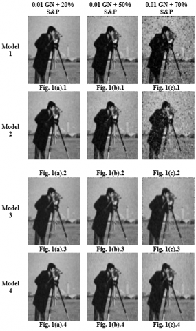
Figure 1. Simulation results of Model 1 to Model 4 at 20%, 50% and 70% salt and pepper and 0.01 variance Gaussian noise
Table 1. PSNR
|
Models/Noise Density |
PSNR |
||
|
0.01 GN + 20% S&P |
0.01 GN + 50% S&P |
0.01 GN + 70% S&P |
|
|
Model 1 |
25.1796 |
23.9368 |
19.5779 |
|
Model 2 |
25.1813 |
23.9371 |
20.0799 |
|
Model 3 |
23.0723 |
22.6183 |
21.8030 |
|
Model 4 |
24.5349 |
23.6948 |
22.0810 |
Table 2. SSIM
|
Models/Noise Density |
SSIM |
||
|
0.01 GN + 20% S&P |
0.01 GN + 50% S&P |
0.01 GN + 70% S&P |
|
|
Model 1 |
0.7574 |
0.6981 |
0.4958 |
|
Model 2 |
0.7588 |
0.6853 |
0.4930 |
|
Model 3 |
0.6916 |
0.6710 |
0.6447 |
|
Model 4 |
0.7300 |
0.6985 |
0.6478 |
Table 3. Simulation time
|
Models/Noise Density |
Simulation* time in Seconds |
||
|
0.01 GN + 20% S&P |
0.01 GN + 50% S&P |
0.01 GN + 70% S&P |
|
|
Model 1 |
1.323 |
1.398 |
1.402 |
|
Model 2 |
1.352 |
1.378 |
1.398 |
|
Model 3 |
0.533 |
0.583 |
0.459 |
|
Model 4 |
1.385 |
1.755 |
1.863 |
*The Simulations are carried in Matlab R2023b
Table 4. PSNR
|
Models/Noise Density |
PSNR |
||
|
0.01 GN + 20% S&P |
0.1 GN + 20% S&P |
0.25 GN + 20% S&P |
|
|
Model 1 |
25.2150 |
19.1375 |
12.0133 |
|
Model 2 |
25.1921 |
19.0210 |
11.9645 |
|
Model 3 |
23.1009 |
18.4829 |
12.3963 |
|
Model 4 |
24.4640 |
18.8941 |
12.3261 |
In Figure 1, the performance of these models is analyzed at different noise levels of mixed noise (salt and pepper (S&P) plus Gaussian noise (GN)). The number of iterations is chosen as 10. In Figure 1(a)-1(c), Gaussian noise of variance 0.01 plus salt and pepper noise of noise densities of 20%, 50%, and 70% is added, respectively. As per the quantitative analysis, the performance of all four proposed models is almost similar and satisfactory in terms of PSNR and SSIM (Tables 1-2). Watching closely the PSNR and SSIM, it is clear that the Model 1 and Model 2 performances are better in comparison with Model 3 and Model 4 at low and medium noise densities. Model 4 outperforms all other models at high noise density. From the qualitative and quantitative analysis of Figure 1, it is clear that mixed noise is removed in all four models with good edge preservation. The simulation taken for each model is shown in Table 3.
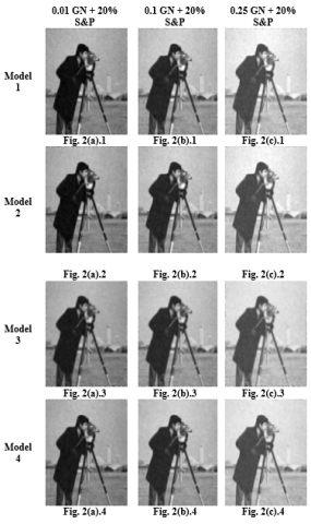
In Figure 2, the performance of all four models is analyzed at different Gaussian noise variances plus a fixed salt and noise density. From Figures 2(a)–2(c), the Gaussian noise variance is 0.01, 0.1, and 0.25, respectively, with a fixed salt and noise density of 20%. The corresponding performance metrics are shown in Table 4 and Table 5. The simulation time taken for these models is shown in Table 6. It is clear from Figure 2, Table 4, and Table 5 that the performance of all the models is satisfactory at various levels of Gaussian noise, although the performance is better at a low Gaussian noise variance of 0.01 (Figure 2(a)). A keen analysis of the performance metrics (Table 4 and Table 5) shows that Model 1 performance is slightly better as compared to the remaining three models.
Figure 2. Simulation results of Model 1 to Model 4 at 20% salt and pepper and Gaussian noise of variance 0.01, 0.1 and 0.25
Table 5. SSIM
|
Models/Noise Density |
SSIM |
||
|
0.01 GN + 20% S&P |
0.1 GN + 20% S&P |
0.25 GN + 20% S&P |
|
|
Model 1 |
0.7603 |
0.6898 |
0.6114 |
|
Model 2 |
0.7585 |
0.6892 |
0.6123 |
|
Model 3 |
0.6914 |
0.6518 |
0.5853 |
|
Model 4 |
0.7281 |
0.6841 |
0.6070 |
Table 6. Simulation time
|
Models/Noise Density |
Simulation* Time in Seconds |
||
|
0.01 GN + 20% S&P |
0.1 GN + 20% S&P |
0.25 GN + 20% S&P |
|
|
Model 1 |
1.340 |
1.370 |
1.425 |
|
Model 2 |
1.374 |
1.424 |
1.443 |
|
Model 3 |
0.521 |
0.610 |
0.621 |
|
Model 4 |
1.421 |
1.451 |
1.472 |
*The Simulations are carried in Matlab R2023b
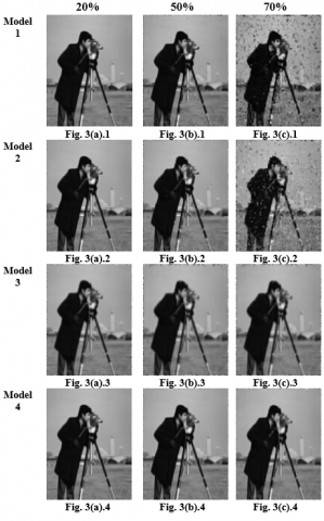
Figure 3. Simulation results of Model 1 to Model 4 at 20%, 50% and 70% salt and pepper noise densities
Table 7. PSNR
|
Models/Noise Density |
PSNR |
||
|
20% S&P |
50% S&P |
70% S&P |
|
|
Model 1 |
25.8899 |
24.8335 |
20.3033 |
|
Model 2 |
25.9483 |
25.0511 |
21.3970 |
|
Model 3 |
24.2123 |
23.8080 |
22.9530 |
|
Model 4 |
26.1375 |
25.3888 |
23.7741 |
Table 8. SSIM
|
Models/Noise Density |
SSIM |
||
|
20% S&P |
50% S&P |
70% S&P |
|
|
Model 1 |
0.8128 |
0.7779 |
0.5951 |
|
Model 2 |
0.8124 |
0.7771 |
0.6121 |
|
Model 3 |
0.7499 |
0.7350 |
0.7180 |
|
Model 4 |
0.8090 |
0.7835 |
0.7506 |
The performance of the four models under the perturbation of salt and pepper noise alone at different noise densities of 20%, 50%, and 70% is shown in Figure 3. The corresponding performance metrics are shown in Tables 7 and 8. From Figure 3, it is clear that all four models are suited for low and medium noise densities (Figure 3(a) and Figure 3(b)). The performance of Model 3 and Model 4 is good even at a high noise density of 70% (Figure 3(c)-3 and Figure 3(c)-4). The Model 4 outperforms all the models at all levels of noise densities.
Four foundational diffusion smoothing algorithms are discussed and compared. A unified model for the diffusion-smoothing class of algorithms is proposed. The four foundational diffusion algorithms are expressed in accordance with the unified model. Four new models, Model 1, Model 2, Model 3, and Model 4, in accordance with the unified model, are proposed for the removal of mixed noise. The qualitative and quantitative performances of the four models are analyzed. The unified model can serve as the basis for the development of any diffusion smoothing filter. Different diffusion smoothing filters for the removal of different types of noise can be developed in accordance with the unified model. The unified model can serve as a basis for the development of new diffusion smoothing filters for several applications under the perturbation of different types of noise. Diffusion smoothing filters for the removal of different types of noise can be developed in accordance with the unified model by appropriately choosing the statistical estimation operation and the operations on the preprocessing or postprocessing stage. Developing a diffusion smoothing filter in accordance with the unified model for the diffusion smoothing of satellite images under the perturbation of speckle noise can be considered a future work.
[1] Manikandan, S., Ebenezer, D. (2008). A nonlinear decision-based algorithm for removal of strip lines, drop lines, blotches, band missing and impulses in images and videos. EURASIP Journal on Image and Video Processing, 2008: 1-10. https://doi.org/10.1155/2008/485921
[2] Srinivasan, K.S., Ebenezer, D. (2007). A new fast and efficient decision-based algorithm for removal of high-density impulse noises. IEEE Signal Processing Letters, 14(3): 189-192. https://doi.org/10.1109/LSP.2006.884018
[3] Jayaraj, V., Ebenezer, D. (2010). A new switching-based median filtering scheme and algorithm for removal of high-density salt and pepper noise in images. EURASIP Journal on Advances in Signal Processing, 2010: 1-11. https://doi.org/10.1155/2010/690218
[4] Babaud, J., Witkin, A.P., Baudin, M., Duda, R.O. (1986). Uniqueness of the Gaussian kernel for scale-space filtering. IEEE Transactions on Pattern Analysis and Machine Intelligence, (1): 26-33. https://doi.org/10.1109/TPAMI.1986.4767749
[5] Perona, P., Malik, J. (1990). Scale-space and edge detection using anisotropic diffusion. IEEE Transactions on Pattern Analysis and Machine Intelligence, 12(7): 629-639. https://doi.org/10.1109/34.56205
[6] Black, M.J., Sapiro, G., Marimont, D.H., Heeger, D. (1998). Robust anisotropic diffusion. IEEE Transactions on Image Processing, 7(3): 421-432. https://doi.org/10.1109/83.661192
[7] Ling, H., Bovik, A.C. (2002). Smoothing low-SNR molecular images via anisotropic median-diffusion. IEEE Transactions on Medical Imaging, 21(4): 377-384. https://doi.org/10.1109/TMI.2002.1000261
[8] Ham, B., Min, D., Sohn, K. (2012). Robust scale-space filter using second-order partial differential equations. IEEE Transactions on Image Processing, 21(9): 3937-3951. https://doi.org/10.1109/TIP.2012.2201163
[9] Khan, N.U., Arya, K.V., Pattanaik, M. (2014). Edge preservation of impulse noise filtered images by improved anisotropic diffusion. Multimedia Tools and Applications, 73(1): 573-597. https://doi.org/10.1007/s11042-013-1620-8
[10] Tian, H., Cai, H., Lai, J. (2014) A novel diffusion system for impulse noise removal based on a robust diffusion tensor. Elsevier Neurocomputing, 133: 222-230. https://doi.org/10.1016/j.neucom.2013.11.014
[11] Li, S., Zhi, Z. (2020). A novel nonlinear second order hyperbolic partial differential equation-based image restoration algorithm with directional diffusion. IEEE Access, 8: 131021-131031. https://doi.org/10.1109/ACCESS.2020.3010031
[12] Marami, B., Scherrer, B., Afacan, O., Erem, B., Warfield, S.K., Gholipour, A. (2016). Motion-robust diffusion-weighted brain MRI reconstruction through slice level registration-based motion tracking. IEEE Transactions on Medical Imaging, 35(10): 2258-2269. https://doi.org/10.1109/TMI.2016.2555244
[13] Tian, C., Chen, Y. (2020). Image segmentation and denoising algorithm based on partial differential equations. IEEE Sensors Journal, 20(20): 11935-11942. https://doi.org/10.1109/JSEN.2019.2959704
[14] Luo, K., Wang, B., Guo, N., Yu, K., Yu, C., Lu, C. (2020). Enhancing SNR by anisotropic diffusion for Brillouin distributed optical fiber sensors. Journal of Lightwave Technology, 38(20): 5844-5852. https://doi.org/10.1109/JLT.2020.3004129
[15] Yao, Y., Roxas, M., Ishikawa, R., Ando, S., Shimamura, J., Oishi, T. (2020). Discontinuous and smooth depth completion with binary anisotropic diffusion tensor. IEEE Robotics and Automation Letters, 5(4): 5128-5135. https://doi.org/10.1109/LRA.2020.3005890
[16] Guo, F., Zhou, C., Liu, W., Liu, Z. (2022). Pixel difference function and local entropy-based speckle reducing anisotropic diffusion. IEEE Transactions on Geoscience and Remote Sensing, 60: 1-16. https://doi.org/10.1109/TGRS.2022.3182886
[17] Liang, L., Jin, L., Xu, Y. (2022). PDE learning of filtering and propagation for task-aware facial intrinsic image analysis. IEEE Transactions on Cybernetics, 52(2): 1021-1034. https://doi.org/10.1109/TCYB.2020.2989610
[18] Yang, J.B., Guo, Z.C., Wu, B.Y., Du, S. (2023). A nonlinear anisotropic diffusion model with non-standard growth for image segmentation. Applied Mathematics Letters, 141: 108627. https://doi.org/10.1016/j.aml.2023.108627
[19] Du, Z.J., He, C.J. (2023). Anisotropic diffusion with fuzzy-based source for binarization of degraded document images. Applied Mathematics and Computation, 441: 127684. https://doi.org/10.1016/j.amc.2022.127684
[20] Yang, J.B., Guo, Z.C., Zhang, D.Z., Wu, B.Y., Du, S. (2022). An anisotropic diffusion system with nonlinear time-delay structure tensor for image enhancement and segmentation. Computers & Mathematics with Applications, 107: 29-44. https://doi.org/10.1016/j.camwa.2021.12.005
[21] Choudhury, A.P., Halder, T., Gayen, R.K., Ray, A.M., Chakravarty, D. (2022). C-band and L-band AirSAR image fusion technique using anisotropic diffusion. Materials Today: Proceedings, 58(1): 433-436. https://doi.org/10.1016/j.matpr.2022.02.393
[22] Hayes, M.H. (2011). Statistical Digital Signal Processing and Modelling. John Wiley & Sons Inc., Wiley-India ed.