Saurav Ganguly*![]() | Ishita Ghosh
| Ishita Ghosh![]() | Puli Kishore Kumar
| Puli Kishore Kumar![]() | Indranil Sarkar
| Indranil Sarkar![]() | Jayanta Ghosh
| Jayanta Ghosh![]() | Mainak Mukhopadhyay
| Mainak Mukhopadhyay![]()
© 2024 The authors. This article is published by IIETA and is licensed under the CC BY 4.0 license (http://creativecommons.org/licenses/by/4.0/).
OPEN ACCESS
In the domain of array signal processing, the identification and suppression of jamming signals pose significant challenges, particularly in scenarios where intentional interferers operate in the far-field region. This study introduces an innovative beamforming technique, the multi-target least square constant modulus algorithm (MT-LSCMA), which surpasses traditional direction-of-arrival (DOA) estimation methods like estimation of signal parameters via rotational invariant techniques (ESPRIT) and multiple signal classification (MUSIC) by addressing their limitations in computational complexity, detection efficacy, and inaccuracies arising from coherent sources. Unlike conventional approaches, the MT-LSCMA, an extension of the blind constant modulus adaptive beamforming method, does not rely on a reference signal for the optimization of the mean-square-error (MSE) cost function. Instead, it iteratively updates the weights based on constant modulus signal information, facilitating the identification of jammer locations even under low signal-to-noise ratios (SNR). This methodology enhances anti-jamming capabilities by adaptively forming nulls in the radiation pattern directed towards the jammers. Simulation results demonstrate the superior accuracy of the MT-LSCMA in tracking jammers compared to both traditional and recently developed techniques. The proposed method yields significant improvements in detection probability, resolution probability, failure rate, computational complexity, and root-mean-square-error (RMSE), thus offering a robust solution for effective jammer location identification and suppression.
constant modulus algorithm (CMA), direction-of-arrival (DOA) estimation, intentional interferers, jamming signal suppression, least square constant modulus algorithm (LSCMA), null steering, root mean square error (RMSE)
Refuting intentional interference or mitigation of jamming signals has continued to be a major challenge for wireless communication and radar researchers for years [1-8]. Jamming remains a considerable threat to applications that go through space-time processing [5-8]. Jammers are used intentionally in radio communication to deliberately block and disrupt the communication channel, typically by reducing the SNR. Consequently, familiarity of specific localization of intentional jammers is of utmost importance to radio engineers and researchers at low SNR values, so as to mitigate and reduce the effect of interfering signals.
In the entire procedure of jamming signal mitigation, the detection of the location of the jammer constitutes an important and primary step. Jammer locations can be precisely identified by estimating the DOA of the jamming signals impinging on an array of antennas or sensors with some array processing capabilities. Traditional strategies for estimating DOA, such as MUSIC [9] or a variant of ESPRIT [10-14], make use of isotropic sensors or omnidirectional antenna elements of dense uniform linear array (ULA) to form and decompose a square array correlation matrix of the impinging signals. Other than settling with a lesser degree of freedom (DOF), a major disadvantage of the conventional DOA estimation methods is their failure to resolve near-correlated jamming sources [11-13, 15-17]. Thus, there always remains a possibility of detecting an incorrect number of jammers whose spatial separation is narrow. Eventually, this affects the mitigation process or the null steering of the antenna array beam.
Various solutions have been proposed by researchers over the years for the detection and mitigation of jamming signals. The authors [1-8] utilized either the time, frequency, or space domains, or a combination of all domains, to exploit the detection and mitigation methods. Striking drawbacks evident in time domain and frequency domain processing are performance deterioration in tracking, inaccurate correlation peaks, and acquisition issues [2-5].
1.1 Related works
In the space domain, as spatial mitigation is employed, the performance gets significantly improved [1, 6]. Space domain processing has the potential to estimate the DOA of the impinging signals, then direct the main lobe towards the location of the signal-of-interest (SOI) (or beam-steering) and place nulls in the estimated direction of jamming signals (or null-steering) [18-21]. A smart antenna system may be used to realize space-domain processing. Typically, a smart antenna system consists of an array of sensors with an adaptive signal processing capability that can successfully accomplish null-steering and beam-steering [12, 14, 16]. Of the exclusive two categories well explored, the blind class of adaptive beam-forming algorithms invariably has certain edge over non-blind classifications, as the obligatory learning signal is not necessary, thus improving the system's spectrum efficiency. The most illustrative of the blind adaptive beam-forming methods is the CMA [22]. It is an iterative method that conserves the envelope of the beam-forming response almost at a constant level so as to separate the SOI from the interference. But at low SNR values, CMA fails to resolve the interference signal with the SOI if the interference signal stringently follows the constant modulus property. This issue can be sorted out to some degree by using the least squares approach, minimizing the cost function of the CMA over one block of data vectors, and then updating block-by-block. The resulting block iterative method is the LSCMA [14, 23, 24], which acquires better global stability and a faster convergence rate as compared to conventional CMA.
Direction finding based on the paradigm of compressive sensing (CS) structure has garnered considerable interest among researchers in the last decade [25-37]. It provides a different perspective to regenerate the original signal with sparsity characteristics by appending a high reconstruction class at the sensing phase and at the receiver phase, respectively. From 2004 onwards, a group of researchers published a succession of research papers in which it was conclusively proved that exact reconstruction of a signal is conceivable with fewer samples than the Nyquist rate necessitates, provided that some statistics of the sparsity characteristics of the signal are known beforehand. This concept led to the development of the theory of CS in signal processing [25-27, 34].
The achievement of CS-based sparse reconstruction is established on two basic properties of the intended signal: compressed or sparse representation and incoherency [25-27]. In source localization problems, in which the DOA of the impinging signals is estimated, the sparsity or compressed representation is guaranteed by making use of a suitable angular transformation. The framework of CS provides a distinguishing edge over the standard models of AOA estimation in reduced computational complexity, reconstruction by single snapshot, and improved degrees of freedom [27-30].
The general development of sparse signal classification for DOA estimation in the CS domain is well studied in several literatures [26-30, 34]. The single snapshot recovery issue is effectively addressed in several literatures [26, 27, 30, 35], while multiple-time snapshot-based DOA is being estimated and studied in the literature [28], exhibiting promising resolution characteristics. In the literature [29], various optimization algorithms based on $\ell_0, \ell_1$ and $\ell_2$ norms for direction finding are examined, and performances are being compared in terms of computational complexity, mean-square error, resolution, and recovery time. The problem of random selection of sensors and the pair-matching issue in 2-D DOA estimation by an L-shaped array are well studied in several literatures [31-33]. Instead of a ULA, a co-prime array structure is effectively used in the CS paradigm for estimating the DOA of the receiving signals in several literatures [36, 37]. One of the major advantages of the co-prime array structure is that it provides a larger array aperture as compared to ULA, which enables better resolution in DOA estimation problems.
In recent years, a deep learning framework has been introduced by researchers for identifying a specific signal direction from multiple signals impinging on an array of antennas [38-41]. Both 1-D and 2-D DOA estimation parameters are studied in ULA, uniform circular array (UCA), and retro-directive arrays (RDA), respectively. In deep learning models, improved resolution is obtained as the network does not depend on the statistical properties of the signal.
Contemporary developments in DOA estimation, as discussed, have revealed striking advantages over standard models, particularly in obtaining enhanced degrees of freedom, lower computational complexity, a single snapshot instance, and more accurate resolution for near-coherent targets. But the requirements of the training data and the decision and construction of the sensing matrices remain prominent hindrances in both deep learning and sparse reconstruction methods. Also, finding the location of an interferer or jammer and being able to steer nulls of the antenna array beam, when the SNR is low have not been studied or talked about much in recent research.
The main aim of this paper is to introduce a novel high-resolution DOA estimation method for the jammer signals at low SNR estimates that are nearly correlated with each other and null-steer the smart antenna system so as to suppress or mitigate the jamming directions effectively. The MT-LSCMA, which is a variant of the LSCMA algorithm, is a robust adaptive beam-forming method that is well exploited in separating the multipath signals from the SOI [42]. The jamming and the SOI sources or targets are assumed to be located in the far-field region with respect to the ULA-based smart antenna receiver, and the narrowband signals impinge on the ULA indiscriminately from all directions. The intrinsic characteristics of the MT-LSCMA are effectively used to create two groups of adaptive weights to distinguish between the jamming signals and the SOI, so as to beam-steer the main lobe on the way to the direction of the SOI and null-steer by inserting nulls in the direction of the jamming signals. The weights of the steering vector are calculated through a novel iterative methodology that results in highly precise DOA estimation. The suggested method can clearly resolve closely spaced DOAs of jamming signals as well as DOAs of signals of interest with the DOAs of the jammers, which makes the antijamming effect stronger. Furthermore, it is capable of improving the null-steering process and avoiding SOI signal level drops while rejecting jamming signals.
The effectiveness of the proposed approach is evaluated and compared with the conventional MUSIC [9] algorithm, the recently developed modified MUSIC (M-MUSIC) [43] algorithm, and CS-based DOA estimation for randomly selected sensors of a ULA [35] and a sparse coprime array [37] in terms of RMSE, resolution probability with varying SNR, and computational complexity. The M-MUSIC algorithm employs the block adaptation method, similar to the proposed technique here. Consequently, the suggested methodology has a faster convergence speed as compared to the MUSIC algorithm. Investigations are accomplished for single and multiple highly correlated jamming signals. Simulation findings show that the proposed approach can determine the jammer locations more accurately at low values of SNR and performs better in terms of probability of detection, failure rate, RMSE, and resolution probability, therefore enhancing the general system performance.
This is how the rest of the paper is structured. Section 2 introduces the system modeling of the DOA estimation problem, while Section 3 provides a brief description of the conventional MUSIC and the M-MUSIC algorithms. In Section 4, the formation of CS-based array pattern reconstruction for DOA estimation from randomly selected sensors of a ULA and a co-prime array structure is discussed. The proposed jammer mitigation algorithm based on MT-LSCMA is developed in Section 5. Section 6 accords with the simulation results and performance comparisons with respect to RMSE, computational complexity analysis, probability of resolution, etc. The paper is completed by the conclusion in Section 7.
Notations: N indicates the total number of antenna elements in a ULA. It is assumed that there are k and i targets or sources (SOI and jammers respectively) located in the far-field region of the ULA. It is necessary to estimate the locations of the jammers. In the first step, the elevation angle or DOA of the target locations (SOI and jammers) are represented by θi and θk respectively. Bold upper- and lower-case symbols represent matrices and vectors respectively. For instance, a(θi,k) represents the array steering vector while A(θi,k) signifies the array manifold matrix. (.)T and (.)H signify vector and Hermitian transpose apiece. All other notations are made acquainted as and when required in the text.
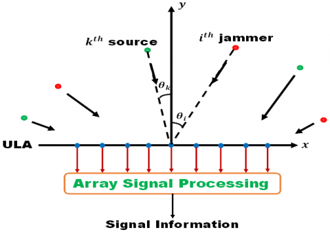
Figure 1 exhibits the basic structure of array signal processing. Multiple targets or sources that are in the far-field region emit propagating waves that impinge on the antenna array from different angular directions in the form of plane waves, as shown. In the far-field region, the antenna array radiation pattern is independent of the distance from the array, and the direction of propagation of the signals is in the form of plane waves.
Figure 1. A basic array signal processing model
Algorithms appropriate for array signal processing are applied to the antenna array output, by which some information about the sources can be deduced, like source direction (or DOA), distance between the targets and the antenna array, velocity of the targets, etc. The targets can be radio sources (or quasi-stationary objects from which RF signals are reflected) or intentional jammers placed ingeniously (shown by green and red points, respectively). The distances between the targets and the antenna array are sufficient (far-field distance), so that the wavefronts can be approximated by plane waves.
The formation of the antenna array is ULA in nature, whose elements are assumed to be isotropic, and the interelement spacing is optimized at d=λ⁄2, where λ is the wavelength of the impinging signals (shown by blue points). This spacing benefits from reducing the spatial aliasing and the mutual coupling effect between the antenna elements. It is assumed that the medium through which the signals propagate and impinge on the array is homogenous and non-dispersive in nature. Also, each element of the antenna array is considered to be isotropic and has no preferred direction of radiation, i.e., it radiates consistently in all directions over a sphere centered on the origin or source.
The main aim of the DOA estimation methodology is to determine a function that provides an implication of the impinging DOA on an array of sensors based on a plot between the maxima and angular values. This functional plot is known as the pseudospectrum P(θ) is dependent on the angle of arrival. One of the best approaches to defining pseudospectrum is by minimizing the mean-squared error of the correlation matrix, formed by the array output, by eigenvalue decomposition. This gives rise to the MUSIC algorithm, developed by Schmidt [9]. It is a subspace-based method, as it specifically exploits the noise subspace. This approach has been found to work effectively for uncorrelated impinging signals as well as noise and has established itself as one of the most popular solutions to the DOA estimation problem. However, for highly correlated impinging signals, MUSIC fails to separate noise as the source correlation matrix becomes singular, and the estimation method breaks down considerably. Besides, due to eigenvalue decomposition, the computational complexity is high and becomes exorbitant for a large sensor or antenna array.
This weakness of the MUSIC algorithm is tackled and substantially reduced in the M-MUSIC technique by exploiting the Nyström method to approximate the noise subspace [43]. A computationally more efficient variant of MUSIC, M-MUSIC is founded on the randomly selected sensor array output. The eigenvalue decomposition of the array correlation matrix is obtained by the Nyström approximation for reconstructing the corresponding noise subspace. Finally, the modified pseudospectrum function is modeled, from which the DOAs are estimated. Consequently, the computational efficiency of M-MUSIC is well established due to the use of smaller array correlation matrices (for randomly chosen small arrays), which reduces eigenvalue decomposition complexities. However, if the original sensor array itself is small-scale, the computational efficiency of M-MUSIC reduces.
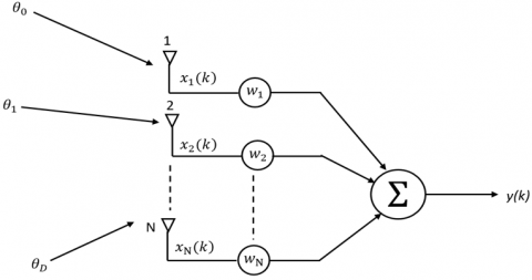
Figure 2. N- element array with impinging signals. Example of spatial filtering
Figure 2 shows a spatial filter with an antenna array of N isotropic components with N prospective weights. D narrowband signals (SOI and jamming signals), originating from the far-field region, impinge on the array from D directions as shown. It is assumed that D<N. Each received signal xi(k) consists of additive white Gaussian noise (AWGN) with a zero mean. The array output at the k-th snapshot can be written as:
$y(k)=\boldsymbol{w}^T . \boldsymbol{x}(k)$ (1)
where, w=[w1 w2 w3……wN]T is the array weight vector.
$\boldsymbol{x}(k)=\left[\boldsymbol{a}\left(\theta_1\right) \boldsymbol{a}\left(\theta_2\right) \boldsymbol{a}\left(\theta_3\right) \ldots .. \boldsymbol{a}\left(\theta_D\right)\right] .\left[\begin{array}{c}s_1(k) \\ s_2(k) \\ \vdots \\ s_D(k)\end{array}\right]+\boldsymbol{n}(k) \Rightarrow \boldsymbol{x}(k)=\boldsymbol{A}(\theta) . \boldsymbol{s}(k)+\boldsymbol{n}(k)$ (2)
where, s(k) is the impinging narrowband signal vector, n(k) is the zero mean, and $\sigma_n^2$ variance AWGN vector, a(θi) is the N-element array steering vector for DOA θi, and A(θ)=[a(θ1) a(θ2) a(θ3) …a(θD)]N×D is the array manifold matrix of the steering vectors a(θi).
For the conventional MUSIC algorithm [9, 14], the correlation matrix is formed by using Eq. (2) as:
$\boldsymbol{R}_{x x}=\boldsymbol{A}(\theta) . \boldsymbol{R}_{s s} . \boldsymbol{A}(\theta)^H+\boldsymbol{R}_{n n}$ (3)
where, $\boldsymbol{R}_{x x}=E\left[\boldsymbol{x}(k) . \boldsymbol{x}(k)^H\right]$ is the N×N array correlation matrix, $\boldsymbol{R}_{s s}=E\left[\boldsymbol{s}(k). \boldsymbol{s}(k)^H\right]$ is the D×D source correlation matrix and $\boldsymbol{R}_{n n}=\sigma_n^2 \boldsymbol{I}$ is the N×N noise correlation matrix (I is the identity matrix). Due to the fact that MUSIC is a subspace-based approach, it estimates the signal and noise subspaces (ES and EN respectively) by eigenvalue decomposition of $\widehat{\boldsymbol{R}}_{x x}$.
The MUSIC pseudospectrum is given by [9, 42] as:
$P(\theta)=\frac{1}{\left|\boldsymbol{a}(\theta)^H \boldsymbol{E}_N \boldsymbol{E}_N^H \boldsymbol{a}(\theta)\right|}$ (4)
The plot of Eq. (4) generates sharp peaks at the angles of arrival of the impinging signals (D).
The angle estimation of Eq. (4) is recognized to achieve a splendid balance between the complexity of computation and the performance of DOA estimation. Subsequently, the MUSIC algorithm has remained a generally accepted method in practice as well as in the literature as a standard proposition [9-10, 43]. But the MUSIC algorithm is very sensitive to near-correlated targets and model mismatches. Nevertheless, the MUSIC algorithm has stimulated the array processing research community to seek better performance in terms of locating correlated targets with reduced computational complexity.
In M-MUSIC algorithm [43], the Nyström approximation is used to construct a new array correlation matrix $\boldsymbol{R}_{x x N^{\prime}}$ by selecting N' elements at random from N for N'<N. The new correlation matrix is designed as:
$\boldsymbol{R}_{x x N^{\prime}}=E\left[\boldsymbol{x}(k) . \boldsymbol{y}(k)^H\right]=\boldsymbol{A}(\theta) . \boldsymbol{R}_{s s} . \boldsymbol{A}_y(\theta)^H+\sigma^2 \boldsymbol{I}_{N \times N^{\prime}}$ (5)
where, $\boldsymbol{y}(k)=\left[\begin{array}{lllll}y_1 & y_2 & \ldots & \ldots & y_{N^{\prime}}\end{array}\right]$ is the output vector of the randomly chosen N' array elements from x(k), Ay(θ) is the direction matrix or manifold matrix of the observation vector y(k) and $\boldsymbol{I}_{N \times N^{\prime}}$ is the N×N' dimensional matrix, in which the diagonal elements are one and other elements are zero.
Applying Nyström approximation to estimating the noise subspace, $E_{N^{\prime}}$, the eigenvalue decomposition yields: $\boldsymbol{R}_{x x N^{\prime}} . \boldsymbol{e}_y=\lambda_y . \boldsymbol{e}_n$, where en is the approximate principle eigenvector. Following this, the process continues using an approach akin to the MUSIC algorithm in estimating the DOA angle θ.
Eventually, the spectral function in Eq. (4) can be reformed as:
$P(\theta)=\frac{1}{\left|\boldsymbol{a}(\theta)^H\left(\boldsymbol{I}_N-\boldsymbol{E}_{N^{\prime}} \boldsymbol{E}_{N^{\prime}}^H\right) \boldsymbol{a}(\theta)\right|}$ (6)
The DOA of the far-field targets is estimated from the angles related to the plot of D spectral peaks in Eq. (6).
In recent years, CS has materialized as a unique sampling paradigm that permits sparse signal acquisition and reconstruction with fewer measurements, less than the Nyquist rate. It has been extensively proven that signals can be reconstructed at sub-Nyquist sampling rates without any loss of information, on condition that they maintain an adequately sparse representation in some domain and that the measurement approach is appropriately chosen [25-27]. CS has recently been used for DOA estimation, exploiting the fact that a superposition of planar wavefronts resembles a sparse angular power spectrum [26-36].
The sparsity and incoherency are two indispensable characteristics that enable CS to occur between the basis ($\Psi$) and sensing (or observation, $\Phi$) matrices. Sparsity of a signal means the condition or fact of a scanty distribution of values over a bound. If the signal sparsity is known, then it is possible to intuitively reconstruct the signal with a few measurements.
The measurement procedure of CS is conceivable as a linear projection of the signal vector into a set of judiciously selected projection vectors that put together almost each bit of detail present in the signal. Every measurement of the signal ought to provide some global information. The advantage of incoherent measurement is that the entire information content of the signal of interest is obtained by adding together all the bits of information that are provided by each measurement.
In the DOA estimation problem, sparsity is assured in the transformed angular domain, while incoherency can be achieved if the restricted isometric property (RIP) is obeyed [25-27], $\left(1-\delta_k\right)\|x\|_2^2 \leq\left\|\boldsymbol{\Phi}_x\right\|_2^2 \leq\left(1+\delta_k\right)\|x\|_2^2$, where $\delta_k \in[0,1]$, and $\Phi$ is the sensing (or observation) matrix. The symbol $\|.\|_2$ symbolizes the $\ell_2- norm$.
Other than properly incorporating the orthogonal sparsity basis matrix $\Psi$, CS requires two more characteristics for effective performance, viz., (1) the design of the stable sensing (or observation) matrix $\Phi$, and (2) proper optimization of the reconstruction algorithm.
The construction of the sensing (or observation) matrix is an important objective of CS, and it mostly depends on whether the characteristics of the impinging signals are known in advance. The components of $\Phi$ can be constructed using unstructured random distributions such as Bernoulli, uniform, or Gaussian if the features of impinging signals are unknown a priori [37]. The number of array elements, computational complexity, and other factors become significantly better when random distributions are used, but the impact of SNR becomes more prominent on the DOA estimation. This considerably reduces the resolution at low SNR values. Another significant drawback of employing random distributions is the need for large storage capacities. A deterministic sensing matrix may be exploited, provided the characteristics of the impinging signal are known a priori. Typically, it can be an identity matrix whose columns and rows are generated based on the number of array elements.
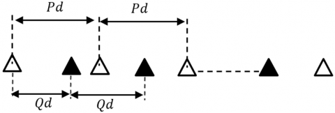
Figure 3. A linear co-prime array structure for DOA estimation
Figure 3 depicts the structure of a co-prime array in 1-D, where P and Q are co-prime numbers. It is created from two dense ULAs, with the number of components in each array as P and Q, respectively, and inter-element spacings as $d=\lambda / 2$.
In the far-field area of a dense ULA and a co-prime array, let us say that the signal sources (or reflected signals) of targets and jammers hit each other as parallel narrowband waveforms. In the single snapshot instance, the received signal vector x[i] of the array (dense ULA or co-prime) is given as in Eq. (2):
$\boldsymbol{x}[i]=\boldsymbol{A}(\theta) \boldsymbol{s}[i]+\boldsymbol{n}[i]$ (7)
where, the symbols and vectors are as described in Eq. (2), page-4 for the ULA. The array steering matrix of the co-prime array configuration is described as:
$\boldsymbol{A}(\theta)=\left[\boldsymbol{a}\left(\theta_1\right), \boldsymbol{a}\left(\theta_2\right), \ldots \ldots \ldots \boldsymbol{a}\left(\theta_K\right)\right] \in \mathbb{C}^{(P+Q-1) \times D}$ (8)
In the CS domain, the received signal vector x[i] from Eq. (7) is compressed to obtain:
$\boldsymbol{y}[i]=\boldsymbol{\Phi} \boldsymbol{x}[i]=\boldsymbol{\Phi}(\boldsymbol{A}(\theta) s[i]+\boldsymbol{n}[i])$ (9)
where, $\Phi$ is the sensing (or observation) matrix of dimension for a dense ULA of elements. For a co-prime array, the dimension of $\Phi$ is M×(N+M-1), where M is the random number of selections or number of measurements of the observation vector y[i].
If the number of sources is known beforehand, then a probable sparse non-convex optimization solution of Eq. (9) is given by:
$\min _{\boldsymbol{y}[i] \in \mathbb{C}^M}\|\boldsymbol{y}\|_0 \,\,subject \,\,to \,\, \boldsymbol{y}[i]=\boldsymbol{\Phi} \boldsymbol{x}[i]$ (10)
The family of matching pursuit reconstruction algorithms, reasonably based on $\ell_0-$ norm, provides the best possible solution to Eq. (10).
5.1 Signal model of LSCM algorithm
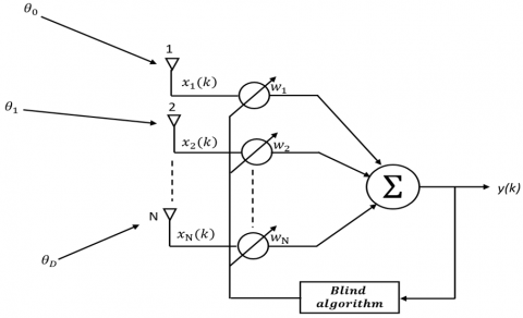
Figure 4. Blind adaptive beamforming method. Example: CMA and its variants like LSCMA and MT-LSCMA
Figure 4 shows a schematic of an adaptive weight updating beamformer with a blind algorithm that generates the error function without the requirement of the desired signal. Blind adaptive spatial filtering is the mathematical basis for the family of CMA and the LSCMA [14, 42]. The cost function of LSCMA using non-linear Gauss’s method is given as [14, 23, 24]:
$J(\boldsymbol{w})=\sum_{k=1}^K|| y(k)|-| \alpha||^2$ (11)
where, α is the array output amplitude. A cost function is an optimizing criterion or performance surface defined based on requirements. In the family of CMA, the minimization of the weighted-sum-of-error-squares criterion is adhered to as an optimizing requirement [23]. The J(w) in Eq. (11) is also known as the dispersion function. This dispersion function (or cost function) can be minimized iteratively by associating the slope of the function with zero. Assuming the narrowband impinging signals (SOI and jammers) are of constant amplitude, Eq. (11) can be re-written as:
$J(\boldsymbol{w})=\sum_{k=1}^K|| y(k)|-1|^2=\left.|| g_k(\boldsymbol{w})\right||_2 ^2=\left.|| g(\boldsymbol{w})\right||^2$ (12)
where, |gk(w)| is the non-linear function of the kth signal and $|.|_2$ is the $\ell_2$ norm. In vector form, |gk(w)| can be expressed as $\boldsymbol{g}(\boldsymbol{w})=\left[g_1(w) g_2(w) \ldots \ldots g_K(w)\right]^T$. Using the offset vector δ, the cost function of Eq. (11) can be expanded by Taylor series as $J(\boldsymbol{w}+\boldsymbol{\delta})=\left\|g(\boldsymbol{w})+\boldsymbol{D}^H(\boldsymbol{w}) \boldsymbol{\delta}\right\|_2^2$, where $\boldsymbol{D}(\boldsymbol{w})=\boldsymbol{\nabla} g_k(\boldsymbol{w})=\left[\nabla\left(g_1(\boldsymbol{w})\right) \nabla\left(g_2(\boldsymbol{w})\right) \ldots \ldots \nabla\left(g_k(\boldsymbol{w})\right]\right.$. Taking the gradient of the expanded cost function and equating it to zero (to achieve the global minima of the error surface), we get:
$\boldsymbol{\delta}=-\left[\boldsymbol{D}(\boldsymbol{w}) \boldsymbol{D}^H(\boldsymbol{w})\right]^{-1} . \boldsymbol{D}(\boldsymbol{w}) \boldsymbol{g}(\boldsymbol{w})$ (13)
If n denotes the iteration number, then the updated weight vector w(n+1) can be generated from Eq. (9) as:
$\begin{gathered}\boldsymbol{w}(n+1)=\boldsymbol{w}(n)-\boldsymbol{D}(\boldsymbol{w}(n)) \boldsymbol{D}^H(\boldsymbol{w}(n))^{-1} \boldsymbol{D}(\boldsymbol{w}(n)) \boldsymbol{g}(\boldsymbol{w}(n)) \\ \Rightarrow \boldsymbol{w}(n)-\left(\boldsymbol{Z} \boldsymbol{Z}^H\right)^{-1} \boldsymbol{Z} \boldsymbol{Z}^H \boldsymbol{w}(n)-\left(\boldsymbol{Z} \boldsymbol{Z}^H\right)^{-1} \boldsymbol{Z} r^*(n) \\ \Rightarrow\left(\boldsymbol{Z Z}^H\right)^{-1} \boldsymbol{Z} r^*(n)\end{gathered}$ (14)
where,
$\boldsymbol{Z}=[z(1) z(2) \ldots \ldots z(K)]^T$ (15)
and r(n) indicates a hard limiter for the operation of y, such that:
$y(n)=\left[\boldsymbol{w}(n)^H \boldsymbol{Z}\right]^T$ (16)
and
$\boldsymbol{r}(n)=\left[\frac{y(1)}{|y(1)|} \frac{y(2)}{|y(2)|} \ldots \ldots \frac{y(K)}{|y(K)|}\right]^T=\boldsymbol{L}(y)$ (17)
The LSCM algorithm is represented by the weight update Eq. (14) and Eqs. (15)-(17). It uses the data block Z(K), and iteration is performed within the block of data to estimate the updated weight vector w(n+1). From the new r(n+1) value, the output y is then calculated. The iteration continues until the weight vector converges.
5.2 MT-LSCM algorithm for location identification and beam-forming
One of the major drawbacks of conventional CMA in direction finding is that their convergence characteristics are highly dependent on the initial values of the weight vector [22, 23, 42]. Thus, there remains a high possibility of convergence at the local minima rather than the true minima point if the initial weight vectors are not chosen appropriately. Consequently, achieving proper minima and convergence criteria is highly sensitive to the initial values of the weight vector.
Also, as the number of array elements or sensors is higher than the number of sources to be detected, it gives rise to different independent beam-forming vectors for an identical output signal [22, 23]. Hence, it is not sufficient to necessitate the independence of the weight vector w. A solution, as proposed [44, 45], supplements the cost function with a term exhibiting independence, but in concurrence with a slower and unpredictable convergence rate [45].
To separate the jamming signal direction from the SOI, the proposed MT-LSCMA resolves two sets of adaptive weights, consequently to null-steer by producing nulls towards the interfering signals and beam-steer the main lobe in the direction of the SOI. The null-steering weights are optimized by MT-LSCMA by $\underset{\boldsymbol{w}}{\operatorname{argmin}}\left\|\boldsymbol{w}^* \widetilde{\boldsymbol{x}}(k)-\boldsymbol{s}(k)\right\|_F$.
From Eq. (1), beam-forming solutions are desirable for known values of either A(θ) or s(k). If A(θ) is known, then the weight vector is set as $\boldsymbol{w}^*=\boldsymbol{A}(\theta)^{\dagger}$, and thus si(k)=w*.x(k). Now, considering that if si(k) is known by apriori, then we set w*=si(k).x(k), with $\boldsymbol{A}(\theta)=\left(\boldsymbol{w}^*\right)^{\dagger}$, where ϯ denotes the Moore-Penrose pseudo inverse. As w*.A(θ)=I attained in both the above cases, the achieved beam-forming exactly cancels all interference.
Now, in the presence of AWGN, the formulation of two sets of linear least-squares minimization models can be put forward. The problems can be either based on minimizing the output error, as:
$\begin{aligned} & \qquad \min _{\boldsymbol{w}, \boldsymbol{s}}\left\|\boldsymbol{w}^* \boldsymbol{x}(k)-\boldsymbol{s}(k)\right\|_F^2 \\ & { such \,\, that \,\, conditions \,\, on }(\boldsymbol{w}, \boldsymbol{s}(k))\end{aligned}$ (18)
or based on minimizing the modelling error, as:
$\begin{gathered}\min _{\boldsymbol{A}, \boldsymbol{s}}\|\boldsymbol{x}(k)-\boldsymbol{A}(\theta) \boldsymbol{s}(k)\|_F^2 \\ { \,\,such \,\,that \,\,conditions \,\,on }(\boldsymbol{A}(\theta), \boldsymbol{s}(k))\end{gathered}$ (19)
For the blind beamforming problem, the signature of the impinging signal is |sij|=1, the constant modulus (CM) condition. Now considering instantanous solution for x(k) in Eq. (2), $\widetilde{\boldsymbol{x}}(k)=\boldsymbol{A}(\theta) . \boldsymbol{s}(k)+\boldsymbol{n}(k)$, the minimization solution of Eq. (15) can be formulated as (if s(k) is known):
$\widehat{\boldsymbol{A}}(\theta)=\underset{\boldsymbol{A}}{\operatorname{argmin}}\|\widetilde{\boldsymbol{x}}(k)-\boldsymbol{A}(\theta) \boldsymbol{s}(k)\|_F^2=\widetilde{\boldsymbol{x}}(k) \boldsymbol{s}(k)^{\dagger}$ (20)
For known values of A(θ), s(k) can be estimated as:
$\boldsymbol{s}(k)=\underset{\boldsymbol{s}}{\operatorname{argmin}}\|\widehat{\boldsymbol{x}}(k)-\boldsymbol{A}(\theta) \boldsymbol{s}(k)\|_{\boldsymbol{F}}^2$ (21)
with the corresponding beam-forming weights as $\boldsymbol{w}=$ $\boldsymbol{A}(\theta)^{\dagger} . \boldsymbol{x}(k)$. Estimated $\widehat{\boldsymbol{A}}(\theta)$ tends to converge to actual values of $\boldsymbol{A}(\theta)$ for noise vector independent of the sources and having zero mean value. The optimization problem of Eq. (14) minimizes the difference of the output signals as:
$\boldsymbol{w}^*=\underset{\boldsymbol{w}}{\operatorname{argmin}}\left\|\boldsymbol{w}^* \widetilde{\boldsymbol{x}}(k)-\boldsymbol{s}(k)\right\|_F^2=\boldsymbol{s}(k) \widetilde{\boldsymbol{x}}(k)$ (22)
Using the identity, $\tilde{\boldsymbol{x}}^{\dagger}=\tilde{\boldsymbol{x}}^*\left(\widetilde{\boldsymbol{x}} \tilde{\boldsymbol{x}}^*\right)^{-1}$, we get:
$\boldsymbol{w}^*=\frac{1}{n} \boldsymbol{s}(k) \widetilde{\boldsymbol{x}}(k)^*\left[\frac{1}{n} \widetilde{\boldsymbol{x}}(k) \widetilde{\boldsymbol{x}}(k)^*\right]^{-1}=\widetilde{\mathcal{R}}_{x x}^{-1} . \widetilde{\mathcal{R}}_{s x}^*$ (23)
where, $\widetilde{\mathcal{R}}_{x x}=\frac{1}{n} \widetilde{\boldsymbol{x}}(k) \widetilde{\boldsymbol{x}}(k)^*$ is the array correlation matrix and $\widetilde{\mathcal{R}}_{s x}=\frac{1}{n} \boldsymbol{s}(k) \widetilde{\boldsymbol{x}}(k)^*$ source-array cross correlation matrix.
Hence,
$\boldsymbol{w} \approx \widetilde{\mathcal{R}}_{x x}^{-1} \cdot \boldsymbol{A}(\theta)$ (24)
Eq. (20) above provides the null-steering weight update solution for MT-LSCMA. With similar considerations, the beam-steering weight update result is derived in the literature [42] as:
$\boldsymbol{w} \approx \boldsymbol{X}^{\dagger}(\boldsymbol{\theta}) . \boldsymbol{S}(\theta)$ (25)
Using Eqs. (22), (23) and (24), the block iterative optimization for null-steering capability of MT-LSCMA can be formulated as:
$\begin{gathered}S(k)^{\prime}=A(k)^{\dagger} \tilde{X} \\ S(k+1)=\boldsymbol{r}_n\left(S(k)^{\prime}\right) \\ A(k+1)=\tilde{X} S(k+1)^{\dagger}\end{gathered}$ (26)
which can be simplified to,
$\begin{gathered}S(k)^{\prime}=w(k)^* \tilde{X} \\ S(k+1)=\boldsymbol{r}_n\left(S(k)^{\prime}\right) \\ w(k+1)^*=s(k+1) \tilde{X}^{\dagger}\end{gathered}$ (27)
with suitable initial values of A(0) and w(0), Eqs. (24), (26) and (27), converge to Wiener solution with descent computational complexity.
In most practical cases, the total number of jammers or interferers to be estimated is less than the number of sensors in the array (N). This leads to a rank deficiency in X=AS. Hence, the beam-forming solution would not be unique. To ensure that the solution would lie in the column span of A, a dimension-reducing prefiltering is performed such that span (F) =span (A), where F is any N×D matrix. Then in the column span of A, all the beam-forming matrices are given by W=FTD×D, where TD×D is a non-singular square matrix for linearly independent beamformers. The noisy pre-filtered data matrix is given by:
$\underline{\tilde{X}}=F^* \tilde{X}$ (28)
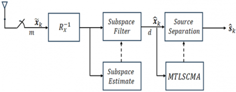
where, $\underline{\tilde{X}}=\underline{A} S+\underline{N}, \underline{A}=F^* A$, and $\underline{N}=F^* N$. The underscored terms denote the pre-filtered variables. Figure 5 depicts a schematic of the MT-LSCMA pre-filtering structure. Prefiltering is an extension of collaborative filtering, which aims at dimensional reduction. The first block, $R_x^{-1}$ performs the whitening of the input coloured noise, and then carry on with the process for the white noise instance. The dimensionality reduction is generally realized by projecting the predictor onto a low-dimensional subspace. The subspace estimator, together with the subspace filter blocks, accomplishes the projection. Finally, blind signal separation with interference is carried out by the proposed method. Commonly, the subspace filter and estimator represent the prefiltering stage.
Figure 5. MT-LSCMA beamforming pre-filtering structure
Table 1 provides a summary of the proposed null-steering based on MT-LSCMA method, as below:
Table 1. Proposed method of jammer direction identification
|
1. Receiving xi(k) as output of each array element from the combined impinging signals, where k denotes the number of snapshots. 2. Formation of a block of impinging data X=[x(1), x(2), …., x(N)]. 3. Determination of the weight update vectors for jammer direction location of MT-LSCMA using Eqs. (20), (22) and (23). 4. Estimation of the array null-steering matrix A=[a(θ1) a(θ2)……. a(θN)]. 5. Estimation of θk from every column vector a(θk) of A, based on the minima of the plot. The null-steering angle is expressed as: $\widehat{\theta}_k=\underset{\theta}{\operatorname{argmin}} \frac{\widehat{a}_k . a(\theta)}{\|a(\theta)\|}$. |
6.1 Parameters used for performance evaluation
The DOA estimation of jammer location and corresponding null-steering capabilities by the proposed MT-LSCMA method are simulated and studied on an experimental testbed using MATLABTM. The effectivity of the proposed methodology is determined and compared with the conventional MUSIC algorithm [9], the newly proposed M-MUSIC algorithm [43], as well as CS framework-based estimation for dense ULA antennas [26, 27, 29, 30] and co-prime array structures [36, 37] for single snapshot circumstances. For all instances, the estimation and reconstruction error or mismatch is calculated by measuring the RMSE at various values of SNR using the Monte Carlo simulation. The measured RMSE for the number MC of Monte Carlo trials is given by [12], which is expressed as the difference between the actual angle θk and the estimated angle of arrival $\hat{\theta}_k$:
$R M S E=\sqrt{\frac{1}{M_C} \sum_{k=1}^{M_C}\left(\hat{\theta}_k-\theta_k\right)^2}$ (29)
The probability of resolution between two jammer targets is defined as [12]:
$P_{\text {res }}=\operatorname{Prob}\left\{\left|\hat{\theta}_k-\theta_k\right| \leq \frac{\Delta \theta}{2}\right\}, k=1 \ldots \ldots m$ (30)
where, $\Delta \theta=\min \left\{\left|\theta_{k 1}-\theta_{k 2}\right|, 1 \leq k_1 \leq k_2 \leq m\right\}$.
Comparisons in terms of computational complexity, probability of detection with respect to SNR, and failure rate are also accomplished in this section.
6.2 Simulation setup
A MATLABTM based testbed is designed, first for a dense ULA and then for a co-prime array, to simulate and test the effectiveness of the suggested methodology with the recently established and conventional models for jammer direction identification and null-steering capabilities.
Far-field narrowband signals are generated (or reflected) from targets (both SOI and jammers) with the center frequency fixed at 3 GHz. These narrowband signals travel as plane waves through a homogenous, non-dispersive medium and impinge on a dense ULA from different directions. The elements of the ULA are assumed to be isotropic in nature and have element spacings of d=λ⁄2=0.05 m, so as to optimize between the mutual coupling effect and spatial aliasing. Estimating the DOA of the narrowband impinging signals and subsequent null-steering is performed for jamming signals with the proposed MT-LSCMA algorithm at SNR=0 dB. For performance comparison, the same ULA is used for observing the null-steering capabilities of the MUSIC and M-MUSIC algorithms. The SNR values are varied to compute the RMSE, probability of error (Pres), probability of detection, and failure rate.
In the CS paradigm, the number of impinging signals are to be known a priori (D). Assuming all the impinging signals are generated (or reflected) from jamming sources, grid angles are implemented to discretize the observation area, with a 1° spacing between each grid. It is supposed that the impinging signals fall at the assigned grid (or off-grid) angles only. In this configuration, the approximate sensor elements for sampling are randomly selected from the dense ULA by CS. An independent, identically distributed Gaussian distribution with zero mean and variance 1⁄((N-1)) is used to construct the sensing matrix $\Phi$, where N is the total number of array elements in the dense ULA.
Now, a co-prime array structure is formed (Figure 3), and the DOA of the jamming signals is estimated in the CS framework. In this case, the sensor elements are not chosen randomly but by the co-prime array structure concept. The sensing matrix is generated as $\boldsymbol{\Phi}=\mathbb{C}^{D \times N}$, where D is the number of impinging signals on the array. The broadside angle (θ) for DOA is assumed to be in the range ±180°.
6.3 Simulation results
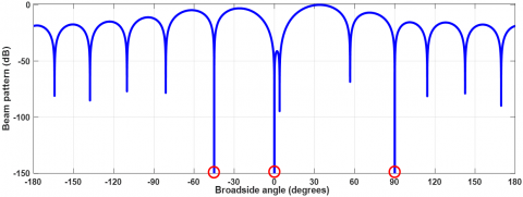
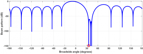
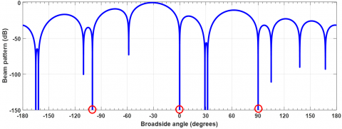
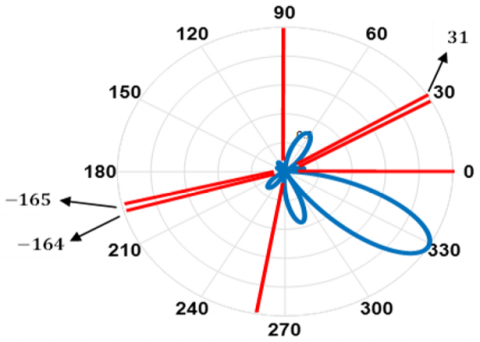
Figure 6 depicts the simulation result of the null-steering capability of the MT-LSCMA for three jammers located in the far-field region, whose reflected signals impinge on a ULA of 13 (N) isotropic elements. The SNR is fixed at 0 dB. The resolution characteristic of the proposed method can be well observed in Figure 7, where three jammer target locations that are closely spaced are null-steered. In Figure 8, multiple jammer locations are identified and null-steered, including targets closely spaced by 1°. In all these simulations, the number of targets (or jammers) is not known a priori. Figure 9 depicts the polar plot of the simulation of identifying and null-steering multiple jammer locations (Figure 8).
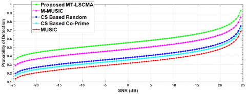
In the second group of simulations, the SNR is varied between ±25 dB (by steps of 5 dB) by keeping the signal power fixed at 0 dB and changing the noise power level. The probability of detection and null-steering towards targets (jammers) in the far-field region is measured and compared with the standard MUSIC, the recently proposed M-MUSIC, and algorithms developed in the CS paradigm (random with ULA and co-prime structure). In the CS paradigm, the number of targets (or jammers) is assumed to be known apriori (D=3). Also, the results are simulated for a single snapshot instance. The probability of detection gives a measure of the ratio between the actual number of detected targets and all possible targets on the deck in a given direction or angular range [13]. Figure 10 shows the comparison result of the detection probability of jammers in the far-field region by varying the SNR values by the proposed MT-LSCMA method, MUSIC, M-MUSIC, CS-based random selection, and CS-based co-prime structure. It is evident from the plot that the proposed method exhibits better detection probability, not only at higher SNR levels but also at lower SNR values.
Figure 6. Plot of beam pattern with angle of arrival for locating jammer directions at -45°, 0° and 90°
Figure 7. Three narrowly located jammers at 35°, 40° and 43°
Figure 8. Location identification of multiple jammers
Figure 9. Polar plot pf Figure 8
Figure 10. Variation of detection probability with SNR (dB)
Figure 11. Variation of root mean square error (RMSE) with SNR (dB)
Figure 12. Variation of probability of resolution with SNR (dB)
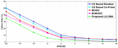
Figure 13. Variation of failure rate with SNR (dB)
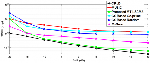
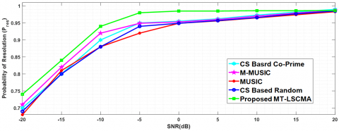
In the third set of simulations, the SNR values are varied between ±20 dB (by similar mode of second group of simulations) and the RMSE eventualized (Eq. (29)) and probability of resolution (Eq. (30)) between the proposed and other methods are compared. The number of Monte Carlo simulations is considered as MC=1000. In CS framework simulations, there is: assumed that D=3 number of targets (or jammers) are known aprioiri and simulations are performed in single snapshot instance.
Figure 11 shows the variation of RMSE with SNR levels, including the plot of Cramer-Rao-Lower-Bound (CRLB). Figure 12 displays the variation of resolution probability with SNR values. Both the simulation outcome confirms the robustness of the proposed methodology in terms of null-steering capabilities.
Figure 13 shows the simulated failure rate comparison with SNR variation with the proposed and other methods. The percentage of unsuccessful trials relative to the total number of trials for the DOA estimation is defined as the failure rate [29]. In this simulation, 1000 number of Monte Carlo trials are considered. In line with the previous configuration, the SNR values were adjusted in steps of 5 dB, ranging from ±20 dB. The simulation results plotted in Figure 13. It is observed that at lower SNR values, the proposed methodology achieves almost 15% less failure index as compared to CS based methods.
6.4 Computational complexity analysis
The complexity of computation is evaluated for the proposed methodology in terms of estimation and null-steering capabilities and compared with the other methods in consideration. As the proposed MT-LSCMA method, together with MUSIC and M-MUSIC, needs to invert the array correlation matrix, the computational involvement tends to be higher than the methods in the CS paradigm.
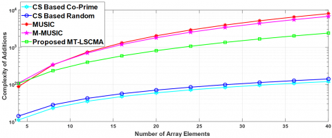
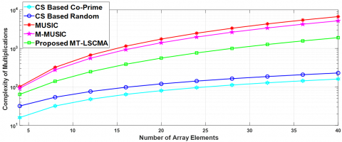
While the array correlation matrix is a N×N square matrix, the computational measurement becomes highly dependent on the structure and number of array elements. For DOA estimation in the CS framework, this dependency is reduced significantly, as the array elements are sparse and either chosen randomly or by co-prime structure. In this set of simulations, the computational measurements are calculated in terms of the number of complex arithmetic operations, i.e., additions and multiplications. Figures 14 (a) and 14 (b) depict the simulation results of the dependency of arithmetical complexity with the number of filter coefficients, or the number of elements in the array structure. The results and the plots clearly show that the complexity of computation is distinctly dependent on the number of array elements, N, particularly for higher numbers. In contrast, methods in the CS paradigm show substantially lower dependency on N, for computational requirements. In terms of matrix inversion methods, the proposed MT-LSCMA approach shows better complexity performance with respect to MUSIC and M-MUSIC algorithms.
6.5 Discussion
Figures 10, 11, and 12 depict the performance comparison of variations in detection probability, RMSE, and probability of resolution with SNR values for the proposed method and other popular standard techniques. In Figure 11, the RMSE values with SNR variation show a promising outcome of the proposed method at SNR values above. Simulation results indicate that the error committed in parametric angular estimation at higher SNR values is comparable with the theoretical bound (Cramér-Rao Lower Bound, or CRLB) of variance (Figure 11). The comparison of detection probability (Figure 10) and resolution probability (Figure 12) parameters shows the better estimation capability of the proposed method even at lower SNR values. Figure 13 depicts that at low SNR values, the proposed method has a 40% lesser failure chance for estimation as compared to other methods.
However, the proposed method requires more additions and multiplications, which makes it more difficult to code than CS methods. This is because correlation matrix inversion is not needed to find the adaptive weights. For large arrays, the computational hazard becomes too complex, as is evident from Figures 14 (a) and 14 (b).
Figure 14 (a). Complexity in terms of additions vs. the length of the array
Figure 14 (b). Complexity in terms of multiplications vs. the length of the array
A new blind adaptive beamforming method is suggested in this paper. It guesses the direction and null-steers towards intentional interferers or jammers in the far-field region. The proposed MT-LSCMA is more noteworthy than its earlier family variants (CMA and others) as it is a block iterative adaptation method and resolves two sets of weights: one for beamforming towards the SOI and the other for null-steering towards the signal-not-of-interest (SNOI) or jammer directions. The null-steering is achieved by optimizing the CMA least squares equation, and the weight update solution is determined by pseudo-inverting the N×N array correlation matrix. Comparing with conventional and popular DOA estimation methods, including the CS paradigm, the proposed method shows more promising results in terms of RMSE, probability of resolution, detection probability, and failure rate, even at lower SNR levels. Higher computational complexity as compared to CS methods is unavoidable due to the requirement of inverting the array correlation matrix. DOA estimation in a CS framework has some clear advantages, such as increased DOFs, single snapshot instances, lower computational complexity, etc. But at lower SNR values, resolution becomes a predominant issue. Simulation results clearly depict that the proposed method works well in terms of probability of resolution, detection probability, failure rate, and RMSE at reduced SNR values as well.
However, all the methods discussed in this paper (proposed MT-LSCMA, conventional MUSIC, M-MUSIC, and CS framework-based) tend to depend highly on the number of array elements while measuring the complexity of computation. The deep learning approach for DOA estimation seems to reduce computational complexity (as the algorithm performance is independent of the physical array structure and array aperture length), which is much lower than the CS paradigm methods but shows inferior resolution at low SNR levels.
The proposed method would find applicability in modern battlefield scenarios, where the noise power is very high, in identifying intentional interferers or jammers in the far-field region with moderate computational complexity. Further, the proposed method can be extended to estimate two-dimensional (2D) DOA estimations of jammer locations comprising both elevation and azimuthal angles. A two-dimensional or planar array would be required for precise estimation of the angle of arrival [31-33].
The simulations are run on a PC with an Intel (R) Core (TM) i7-1165G7 CPU @ 4.6 GHz and 16 GB DDR4 SDRAM using MATLAB R2022b (The MathWorks, Inc., Natick, MA, USA). The operating system is Microsoft Windows 10 Enterprise edition 64-bit.
Conflict of interest: The authors proclaim that they have no competing interest.
[1] Wirth, W.D. (2001). Chapter-10: Adaptive beamforming for jammer suppression, in radar techniques using array antennas. IEE Publishers, London, United Kingdom, pp. 221-252.
[2] Wang, T., Wei, X., Fan, J., Liang, T. (2018). Jammer localization in multihop wireless networks based on gravitational search. Security and Communication Networks, 2018: 7670939. https://doi.org/10.1155/2018/7670939
[3] Nancy, J.T., VijayaKumar, K.P., Kumar, P.G. (2014). Detection of jammer in wireless sensor network. In 2014 International Conference on Communication and Signal Processing, Melmaruvathur, India, pp. 1435-1439. https://doi.org/10.1109/ICCSP.2014.6950086
[4] Xu, W., Ma, K., Trappe, W., Zhang, Y. (2006). Jamming sensor networks: Attack and defense strategies. IEEE Network, 20(3): 41-47. https://doi.org/10.1109/MNET.2006.1637931
[5] Ganeshkumar, P., Vijayakumar, K.P., Anandaraj, M. (2016). A novel jammer detection framework for cluster-based wireless sensor networks. EURASIP Journal on Wireless Communications and Networking, 2016: 1-25. https://doi.org/10.1186/s13638-016-0528-1
[6] Gong, J., Lou, S., Guo, Y. (2018). DOA estimation method of weak sources for an array antenna under strong interference conditions. International Journal of Electronics, 105(11): 1931-1944. https://doi.org/10.1080/00207217.2018.1494324
[7] Mehmood, S., Malik, A.N., Qureshi, I.M., Khan, M.Z.U., Zaman, F. (2021). A novel deceptive jamming approach for hiding actual target and generating false targets. Wireless Communications and Mobile Computing, 2021: 8844630. https://doi.org/10.1155/2021/8844630
[8] Gecgel, S., Goztepe, C., Kurt, G.K. (2019). Jammer detection based on artificial neural networks: A measurement study. In Proceedings of the ACM Workshop on Wireless Security and Machine Learning, pp. 43-48. https://doi.org/10.1145/3324921.3328788
[9] Schmidt, R. (1986). Multiple emitter location and signal parameter estimation. IEEE Transactions on Antennas and Propagation, 34(3): 276-280. http://doi.org/10.1109/TAP.1986.1143830
[10] Roy, R., Paulraj, A., Kailath, T. (1986). Estimation of signal parameters via rotational invariance techniques-ESPRIT. In MILCOM 1986-IEEE Military Communications Conference: Communications-Computers: Teamed for the 90's, Monterey, CA, USA, pp. 41-46. http://doi.org/10.1109/MILCOM.1986.4805850
[11] Godara, L.C. (1997). Application of antenna arrays to mobile communications. II. Beam-forming and direction-of-arrival considerations. Proceedings of the IEEE, 85(8): 1195-1245. http://doi.org/10.1109/5.622504
[12] Van Trees, H.L. (2004). Optimum array processing: Detection, estimation and modulation theory-IV. Hoboken, NJ: Wiley. https://doi.org/10.1002/0471221104
[13] Krim, H., Viberg, M. (1996). Two decades of array signal processing research: The parametric approach. IEEE Signal Processing Magazine, 13(4): 67-94. https://doi.org/10.1109/79.526899
[14] Gross, F. (2015). Smart Antennas with MATLAB. Second Edition, McGraw Hill, New York.
[15] Inzillo, V., De Rango, F., Zampogna, L., Quintana, A.A. (2019). Smart antenna systems model simulation design for 5G wireless network systems. Array Pattern Optim, 1-21. https://doi.org/10.5772/intechopen.79933
[16] Senapati, A., Ghatak, K., Roy, J.S. (2015). A comparative study of adaptive beamforming techniques in smart antenna using LMS algorithm and its variants. In 2015 International Conference on Computational Intelligence and Networks, Odisha, India, pp. 58-62. https://doi.org/10.1109/CINE.2015.21
[17] Bakhshi, G., Shahtalebi, K. (2017). Role of the NLMS algorithm in direction of arrival estimation for antenna arrays. IEEE Communications Letters, 22(4): 760-763. http://doi.org/10.1109/LCOMM.2017.2760253
[18] Li, M., Dempster, A.G., Balaei, A.T., Rizos, C., Wang, F. (2011). Switchable beam steering/null steering algorithm for CW interference mitigation in GPS C/A code receivers. IEEE Transactions on Aerospace and Electronic Systems, 47(3): 1564-1579. http://doi.org/10.1109/TAES.2011.5937250
[19] Li, Q., Wang, W., Xu, D., Wang, X. (2014). A robust anti-jamming navigation receiver with antenna array and GPS/SINS. IEEE Communications Letters, 18(3): 467-470. http://doi.org/10.1109/LCOMM.2014.012314.132451
[20] Arribas, J., Fernandez-Prades, C., Closas, P. (2013). Antenna array based GNSS signal acquisition for interference mitigation. IEEE Transactions on Aerospace and Electronic Systems, 49(1): 223-243. http://doi.org/10.1109/TAES.2013.6404100
[21] Sharma, A., Mathur, S. (2016). Performance analysis of adaptive array signal processing algorithms. IETE Technical Review, 33(5): 472-491. http://doi.org/10.1080/02564602.2015.1088411
[22] Treichler, J., Agee, B. (1983). A new approach to multipath correction of constant modulus signals. IEEE Transactions on Acoustics, Speech, and Signal Processing, 31(2): 459-472. http://doi.org/10.1109/TASSP.1983.1164062
[23] Agee, B. (1986). The least-squares CMA: A new technique for rapid correction of constant modulus signals. In ICASSP'86. IEEE International Conference on Acoustics, Speech, and Signal Processing, Tokyo, Japan, pp. 953-956. https://doi.org/10.1109/ICASSP.1986,1168852
[24] Ganguly, S., Ghosh, J., Kumar, P.K. (2019). Performance analysis of array signal processing algorithms for adaptive beamforming. In 2019 URSI Asia-Pacific Radio Science Conference (AP-RASC), New Delhi, India, pp. 1-6. https://doi.org/10.23919/URSIAPRASC.2019.8738291
[25] Candès, E.J., Wakin, M.B. (2008). An introduction to compressive sampling. IEEE Signal Processing Magazine, 25(2): 21-30. http://doi.org/10.1109/MSP.2007.91473
[26] Shen, Q., Liu, W., Cui, W., Wu, S. (2016). Underdetermined DOA estimation under the compressive sensing framework: A review. IEEE Access, 4: 8865-8878. http://doi.org/10.1109/ACCESS.2016.2628869
[27] Tent Beking, M.V. (2016). Sparse array antenna signal reconstruction using compressive sensing for direction of arrival estimation. Faculty of Electrical Engineering, Mathematics and Computer Science, University of Twente, Master's Thesis. http://purl.utwente.nl/essays/69575.
[28] Ganguly, S., Ghosh, J., Mukhopadhyay, M., Kumar, P. K. (2020). Multi-time snapshot based off-grid DOA estimation of sparse array antennas using mfocuss algorithm. In 2020 URSI Regional Conference on Radio Science (URSI-RCRS), Varanasi, India, pp. 1-4. http://doi.org/10.23919/URSIRCRS49211.2020.9113604
[29] Srinivas, K., Ganguly, S., Kishore Kumar, P. (2022). Performance comparison of reconstruction algorithms in compressive sensing based single snapshot DOA estimation. IETE Journal of Research, 68(4): 2876-2884. https://doi.org/10.1080/03772063.2020.1732840
[30] Fortunati, S., Grasso, R., Gini, F., Greco, M.S., Fortunati, S., Grasso, R., Gini, F., Greco, M.S., LePage, K. (2014). Single-snapshot DOA estimation by using compressed sensing. EURASIP Journal on Advances in Signal Processing, 2014: 1-17. http://doi.org/10.1109/ICASSP.2014.6854009
[31] Gu, J.F., Zhu, W.P., Swamy, M.N.S. (2015). Joint 2-D DOA estimation via sparse L-shaped array. IEEE Transactions on Signal Processing, 63(5): 1171-1182. http://doi.org/10.1109/TSP.2015.2389762
[32] Ganguly, S., Ghosh, J., Srinivas, K., Kumar, P., Mukhopadhyay, M. (2019). Compressive sensing based two-dimensional DOA estimation using L-shaped array in a hostile environment. Traitement du Signal, 36(6): 529-538. https://doi.org/10.18280/ts.360608
[33] Ganguly, S., Sarkar, I., Kumar, P.K., Ghosh, J., Mukhopadhyay, M. (2022). Compressive sensing based 2-D DOA estimation by a sparse L-shaped co-prime array. In 2022 URSI Regional Conference on Radio Science (USRI-RCRS), Indore, India, pp. 1-4. https://doi.org/10.23919/URSI-RCRS56822.2022.10118452
[34] Liu, C.L. (2018). Sparse array signal processing: New array geometries, parameter estimation, and theoretical analysis. California Institute of Technology. Pasadena, California. Doctoral Dissertation. https://resolver.caltech.edu/CaltechTHESIS:05302018-095132389.
[35] Ganguly, S., Ghosh, I., Ranjan, R., Ghosh, J., Kumar, P. K., Mukhopadhyay, M. (2019). Compressive sensing based off-grid DOA estimation using OMP algorithm. In 2019 6th International Conference on Signal Processing and Integrated Networks (SPIN), pp. 772-775. http://doi.org/10.1109/SPIN.2019.8711677
[36] Zhou, C., Gu, Y., Zhang, Y. D., Shi, Z., Jin, T., Wu, X. (2017). Compressive sensing-based coprime array direction-of-arrival estimation. Iet Communications, 11(11): 1719-1724. http://doi.org/10.1049/iet-com.2016.1048
[37] Ganguly, S., Ghosh, J., Kumar, P.K., Mukhopadhyay, M. (2022). An efficient DOA estimation and jammer mitigation method by means of a single snapshot compressive sensing based sparse coprime array. Wireless Personal Communications, 123(3): 2737-2757. https://doi.org/10.1007/s11277-021-09263-9
[38] Elbir, A.M., Mishra, K.V., Eldar, Y.C. (2019). Cognitive radar antenna selection via deep learning. IET Radar, Sonar & Navigation, 13(6): 871-880. http://doi.org/10.1049/iet-rsn.2018.5438
[39] Elbir, A.M. (2020). DeepMUSIC: Multiple signal classification via deep learning. IEEE Sensors Letters, 4(4): 1-4. http://doi.org/10.1109/LSENS.2020.2980384
[40] Nannuru, S., Gerstoft, P., Ping, G., Fernandez-Grande, E. (2021). Sparse planar arrays for azimuth and elevation using experimental data. The Journal of the Acoustical Society of America, 149(1): 167-178. https://doi.org/10.1121/10.0002988
[41] Grumiaux, P.A., Kitić, S., Girin, L., Guérin, A. (2022). A survey of sound source localization with deep learning methods. The Journal of the Acoustical Society of America, 152(1): 107-151. https://doi.org/10.1121/10.0011809
[42] Ganguly, S., Ghosh, J., Kumar, P.K., Mukhopadhyay, M. (2020). An efficient source localization method in presence of multipath using smart antenna system. Journal of Scientific and Industrial Research – NIScPR-CSIR (India), 79(12): 1069-1073. https://doi.org/10.56042/jsir.v79i12.35127
[43] Liu, G., Chen, H., Sun, X., Qiu, R.C. (2016). Modified MUSIC algorithm for DOA estimation with Nyström approximation. IEEE Sensors Journal, 16(12): 4673-4674. http://doi.org/10.1109/JSEN.2016.2557488
[44] Shynk, J.J., Gooch, R.P. (1996). The constant modulus array for cochannel signal copy and direction finding. IEEE Transactions on Signal Processing, 44(3): 652-660. http://doi.org/10.1109/78.489038
[45] Leshem, A., van der Veen, A.J. (2008). Blind source separation: The location of local minima in the case of finitely many samples. IEEE Transactions on Signal Processing, 56(9): 4340-4353. http://doi.org/10.1109/TSP.2008.921721