Sıtkı Akkaya![]()
© 2024 The author. This article is published by IIETA and is licensed under the CC BY 4.0 license (http://creativecommons.org/licenses/by/4.0/).
OPEN ACCESS
In electrical systems, diverse power quality disturbances (PQDs) often contain varying levels of noise, presenting significant challenges in their analysis and classification. This study proposes an innovative approach, employing a convolutional neural network (CNN) optimized in conjunction with wavelet synchrosqueezed transform (WSST) for the efficient detection and classification (D&C) of PQDs. A comprehensive dataset, encompassing 21 hybrid noisy-class instances comprising both singular and multiple PQDs under various noise intensities, was meticulously assembled. These datasets, encompassing time-series signals, were subjected to training and testing on a high-performance workstation using the CNN model, notably without the prerequisite of pre-processing, a deviation from conventional methodologies. The outcomes of this research highlight the substantial efficacy of the optimized CNN model. In environments characterized by a Signal-to-Noise Ratio (SNR) between 20 to 60 dB, the model achieved a peak accuracy of 99.93%. Remarkably, in scenarios with SNR equal to or exceeding 50 dB, the model demonstrated a perfect accuracy rate of 100%. This underscores the robustness of the proposed WSST-enhanced CNN framework, particularly in scenarios plagued with intense noise and diverse PQD classes. The optimization of the CNN model was achieved through an exhaustive exploration of the hyperparameter space within the WSST-based datasets. This methodological approach not only affords high accuracy but also significantly reduces computational load.
power quality disturbances (PQDs), detection and classification (D&C), convolutional neural network (CNN), hyperparameter optimization, time-series signal, wavelet synchrosqueezed transform (WSST)
Power systems are supposed to perform under certain system frequencies and amplitudes, but these items are variable in the field. This situation affects the health, security, and efficiency of the power systems negatively. For this reason, monitoring and assessment of power quality momentarily have great importance. Some standardizations, like IEEE 1159, 1459, etc., propose the detailed properties of these effects and models [1-5]. The disturbances affecting negatively the power systems emerge alone or together in a window as flicker, harmonics, notch, sag, interruption, swell, etc. These occur in the range of a half-cycle to two hours in any interval and magnitude [1, 5]. Fourier transform (FT) is a basic signal processing method to analyze PQD, but it has some problems, like spectral leakage. For this reason, it is recommended to work with windows of 0.2 seconds in the standard of the Electrotechnical Commission, the IEC-61000-4-7 [3]. Thus, minimizing the spectral leakage in Fast Fourier Transform (FFT) for power systems with a fundamental system frequency of 50 Hz allows for working with a frequency resolution of 5 Hz and N = 64 (26) samples per cycle. For this reason, as in some studies in studies [6-11], the sampling frequency is chosen as 3200 Hz in this study, too. The selection of machine learning algorithms’ (MLA) parameters seriously affects the performance of PQD D&C, and then the algorithm's accuracy with the optimum hyperparameters is increased [12].
Measurement of the fundamental frequency, which is sensitive to sag and harmonics, is essential and is estimated with a comb filter-based hybrid system [13]. The presence of interharmonics shows that subharmonics seriously damage the detection, measurement, and analysis of the harmonics [14]. Similarly, the measurement of the flicker is affected by not only low-frequency interharmonics (0.5–35 Hz) but also the subharmonics created by the interactions of these interharmonics with each other [8]. The standard IEC flickermeter cannot detect the flicker effects of high-frequency components that are present in the field. For this reason, the IEC flickermeter ought to be revised for the frequency range of 35 Hz and higher frequencies (from 450 Hz to a few KHz) [15]. The high-frequency interharmonics near the fundamental frequency also have a visible flicker effect but are not detectable by the standard flickermeter of IEC-61000-4-15. This problem was solved with a new flickermeter based on voltage peak detection and a curve compatible with this flickermeter at intervals of 5-95 Hz [6]. Those for only high frequency and the whole frequency, respectively, can be analyzed up to 950 Hz, too [7, 9]. Transient stability can be analyzed with the transient stability boundary, which separates the region as a secure and an unsecured one, by a sparse logistic classifier method. This method is better in comparison with other methods such as k-Nearest Neighbors (kNN), Support Vector Machines, and Linear Logistic Classifiers [16]. The envelope estimation, essential for all the features of the whole disturbance, can be analyzed with the signal geometric properties as well as FFT [17]. A comparative study with different MLAs based on feature selection showed that Random Forest with low-number features has more significant performance than the other MLAs [18]. This study also revealed a time-varying grid-noise effect on the signal of the experimental setup. Adaptive Process Noise Covariance Kalman A filter-based sag disturbance detection method can define the times of start and stop of a sag event and phase jump with the help of the estimated process noise [19]. A method for the detection and characterization of interruption and swell was introduced by using a dataset generated on MATLAB or Simulink [20]. Another signal processing method used for the detection of PQDs is wavelet transform (WT). Although this technique contains some filter banks that make it more robust than FFT, its enhanced versions are now available to increase its precision rate. For neighbor disturbances like sag and interruption, a detection method converting waveforms of PQ into 2D-binary vectors, Deep Learning (DL), and Maximal Overlap Discrete Wavelet Transform (MODWT), has been achieved robustly for a noisy field [21]. So far, the entire study is about analyzing each disturbance in detail. While all this process is applied to each disturbance focally and distinctly, that brings the computational load together. Instead of this long process, there are three-level processes such as detection, classification, and quantification. Detection and classification processes, which are important but time-consuming and hard, have motivated researchers recently.
The single and multiple power measurement parameters are calculated by using the Hilbert transform (HT) and the undecimated wavelet packet transform under the standard IEEE 1459-2010 [22]. This method is also used to evaluate transient and interharmonic disturbances [23]. A hybrid PQD-DC method of Rule-Based Decision Tree and Stockwell Transform (ST) is effective for low-number classes [24]. The improved version of ST, the Discrete Orthogonal ST method, is more capable than the others like the discrete wavelet transform (DWT), short-time Fourier transform (STFT), and ST [25]. A time-frequency-Scale transform method, a Hann window that can operate scaling and shifting, provides noise-immunity classification with a high accuracy rate and a 0.2-sec window length [26]. A method based on the fractional Fourier transform is somewhat better than the ST method for the classification of PQDs [27]. A hybrid method combining the features of ST and HT is effective for complex PQDs [28]. The Volterra series with the Type-2 Fuzzy Logic System with MLAs performs well for PQDs [29]. Another method using dual strong tracking filters and the rule-based Extreme Learning Machine achieves higher performance than other similar methods [30]. The best result of the space comprising some different pairs of signal processing algorithms and MLAs was obtained for kNN+HHT (Hilbert Huang Transform) [31]. The hybrid method of Kalman filter and fuzzy expert system has been studied in limited noisy environments and classes [32]. In a two-level method, Kalman filter-based generalized PQD recognition, fundamental frequency, and amplitudes of the harmonic measurement are made at the first level. In the second one, instantaneous total harmonic distortions and related statistical rates are obtained [33]. The method composed of sparse signal decomposition and decision trees classifies noiseless synthetic high-number classes with relatively low accuracy [34]. The hybrid model, including Multi-Objective Grey Wolf Optimizer, 2D-Riesz Transform, and kNN, has performed higher than the other similar MLA-based hybrid models [35]. The novel method using the reformation of Euler’s rotation hypothesis detailed the PQDs as 3D problems, and this has provided more achievement [36]. The Simple Gated Recurrent Network-based PQD algorithm has higher speed, accuracy, and lower complexity in comparison with the others [37]. Time-Dependent Spectral Featured and Adaptive kNN with Excluding Outliers-based PQD D&C method were proposed in study [38]. The hybrid method of classification of time-series features and the significant zero crossings of derivatives has competitive results on different popular datasets when compared to the widely used MLAs [39]. In most studies, the advantages of some time- and frequency-domain signal processing transform techniques and similar techniques compatible with MLAs were used for the detection and classification of PQDs. An evolving Gaussian fuzzy classification-based model is effective for low-number classes [40]. Another two-level hybrid model, including Variational Mode Decomposition and Detrended Fluctuation Analysis, is more robust than the compared techniques in the study [41]. It is underlined that real-time analysis of the PQD is hard and in a premature stage [33, 42].
In addition to the above, there are some studies based on wavelet transform and CNN for PQDs, as follows: A DWT-based effective feature extraction method for PQD was examined in study [43] in a noise-free environment. Optimum hybrid models, including base-wavelets and MLAs, were searched under noisy cases. It was understood that each MLA should pair a different base wavelet under different cases to gain maximum performance [44]. A 1D and 2D CNN-based hybrid method was performed for synthetic noise in study [45] and found to have more performance but nearly the same complexity when compared with the others. A hybrid model consisting of a temporal convolutional network and a CNN has been performed for different cases in study [46] under noiseless conditions. MODWT and the DL-based hybrid method have been proposed to detect differences between the sag and interruption. A spectrogram- and DL-based PQD D&C method was achieved in study [47] with a low-number class and narrow-range noise. Labeling methods based on DL are proposed, and the results of these studies are promising for low-number classes [48, 49]. An image-based deep learning study was carried out on a synthetic dataset with high accuracy [50]. The bagging LSTM method in study [51] performed with high accuracy for a synthetic high-number-classes dataset. In the study in study [52], a method using a CNN has a high accuracy rate for a noise-free synthetic dataset. Also, this study reveals that the Adam optimizer is more usable than the other optimizers for PQD classification. A hybrid method based on deep learning and 2D scalograms has high accuracy for a synthetic dataset generated in MATLAB or Simulink Simscape due to the IEEE 5 bus [51].
A comprehensive study states the requirement of time-frequency analysis to analyze non-stationary signals in real life. That study comparing time-frequency signal processing methods on biomedical signals shows that the most successful algorithm is Synchrosqueezed Transform (SST) + CNN among all considered methods like FFT, WT, HHT, etc. [53]. This method is declared to be enhanced and applied to other variational signals in different fields for future applications [53]. Power Quality Analysis needs robust time-frequency-based methods like SST and CNN since PQDs have similar characteristics to biomedical ones in terms of time variability, noisiness, and diversity, which require high robustness. For these reasons, an enhanced version of this algorithm, WSST and CNN, is selected to generate time-frequency images from PQD signals in the time domain, and then these images will be utilized to detect and classify them.
As can be seen, the algorithms for the detection and classification of PQDs have been carried out restrictedly with a synthetic dataset, low-number classes, a noiseless environment, pre-processing by data degradation leading to measurement error, etc. For all these boundaries, this paper proposes a PQD D&C method that is robust to noise, effective for high PQD classes, and reduces the process carried out with the optimization of a CNN and WSST. As a result, all of the requirements mentioned earlier will be met. Moreover, according to the best knowledge of the author and as mentioned above, although WSST and CNN are well-known methods, no study has been conducted to obtain the best parameters from the hybrid model created by these methods for the detection and classification of PQDs.
Objective
The primary objective of this research is to develop a hybrid methodology that facilitates rapid and highly accurate detection of PQDs within noisy and dynamically fluctuating power system signals. This approach leverages the combined strengths of CNN and WSST to achieve superior accuracy and robustness in PQD detection.
Contributions
This study makes several significant contributions to the field of power quality analysis:
(1) Data Generation and Preparation:
-Data for this research will be generated entirely at random, adhering to the IEEE 1149 standard.
-The dataset will incorporate noise variably added across a broad spectrum, ranging from 20 to 60 dB.
-A total of 21 distinct PQD classes will be delineated and analyzed.
(2) Innovative Approach:
-This study is pioneering in its use of WSST for the detection of power quality issues.
-It also marks the first instance of a hybrid PQD detection and classification (D&C) method that synergizes the optimization capabilities of both CNN and WSST.
Structure
Section 1 delineates the various PQD classes, elucidated through detailed equations and figures. Sections 2 and 3 provide an in-depth exploration of the WSST technique and CNN algorithms, including an examination of the relevant hyperparameters. In Section 5, the proposed PQD D&C method, which focuses on the Optimization of CNN with WSST, is defined and elaborated upon, incorporating models and block diagrams for clarity. Section 6 presents the numerical results of the study, featuring comparative analyses via figures and tables. Section 7 describes the experimental setup and the process flowchart employed to gather the dataset. Finally, Section 8 discusses the findings of the study and explores potential avenues for future research in this area.
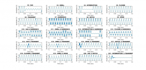
In the IEEE 1159 standard, all models of power quality disturbances and their limitations are given in detail. These models and limitations are characterized by different times, frequencies, and amplitudes. These disturbances, such as interruption, sag, swell, harmonics, flicker, transients, spikes, and notches, emerge single or multiple.
Each PQD labeled in the range from C1 to C21 was defined in Table 1. All the parameters of the classes are generated in a noisy environment in a range of 20 dB to 60 dB randomly according to given standard intervals.
The variable parameters in Table 1, i.e., amplitude, frequency, and time matrices, are given in the following Eqs. (1)-(3). Moreover, the elements of these matrices have also been constructed randomly in the range of intervals given in Table 1 and then waveform datasets prepared accordingly.
$amplitude =\left[\begin{array}{c}{\alpha_{\text {sag }}, \alpha_{\text {swell }}, \alpha_{\text {interruption }}, \alpha_{\text {flicker }}, \alpha_{\text {transient }}} \\ \alpha_3, \alpha_5, \alpha_7, \alpha_{\text {notch }}, \alpha_{\text {spike }}\end{array}\right]$ (1)
$time =\left[t_1, t_2, t_3, t_4, t_5, t_6, \tau\right]$ (2)
$frequency =\left[f_0, f_{\text {flicker }}, f_{\text {transient }}\right]$ (3)
For minimizing spectral leakage, the Electrotechnical Commission in IEC-61000-4-7 recommends working with windows of 0.2 seconds, which provides a 5 Hz resolution for analysis with a 3.2 kHz sampling frequency [3]. For this reason, as in some studies [6-11], this sampling frequency is chosen for this study, too. The other phenomenon, the number of signals, is defined by a relationship among the number of classes (21), the number of noise ranges (9- for 20: 5: 60 dB), and the number of flicker curve frequencies, which is 35 in IEC 61000-4-15 (35). Namely, the sampling frequency, window length, and number of signals are selected as 3.2 kHz, 0.2 s (10 cycles), and 6615 (corresponding to 21x9x35) based on IEC 61000-4-7, 4-15, and IEEE 1459 standards, respectively.
In this study, all time-series PQD signals are generated as models in Table 1. Then the noises are loaded onto these signals in different ranges randomly, too. Owing to the fact that the IEC flicker meter standard has proposed a flicker curve consisting of 35 different frequencies versus amplitudes, this number has been selected as a reference for the research. Similarly, 35 different time-series signals between 20 dB and 60 dB for each class are generated, and thus, a total of 6615 different signals have been made out. Before the CNN training, these signals were transformed by WSST, and so the dataset was converted from 1D to 2D.
All waveform figures except for pure signal C1 are presented for a 60-dB noisy environment in Figure 1. These figures are prepared with reference to Table 1, and the parameters like amplitude, time, and frequency are entirely randomly selected in the given range.
Table 1. Mathematically models and related parameters of power quality disturbances
|
Class |
Type |
Model Equation |
Parameter |
|
C1 |
Pure |
$v(t)=\sin \left(2 \pi f_0 t\right)$ |
$f_0=50 \mathrm{~Hz}$ |
|
C2 |
Sag |
$v_1(t)=\left[1-\alpha_{s a g}\left(u\left(t-t_1\right)-u\left(t-t_2\right)\right)\right] \sin \left(2 \pi f_0 t\right)$ |
$\begin{gathered}0.1 \leq \alpha_{\text {sag }} \leq 0.9 \\T_0 \leq t_2-t_1 \leq 9 T_0 \\T_0=1 / f_0 \\u: \text{unit step function}\end{gathered}$ |
|
C3 |
Swell |
$v_2(t)=\left[1+\alpha_{\text {swell }}\left(u\left(t-t_1\right)-u\left(t-t_2\right)\right)\right] \sin \left(2 \pi f_0 t\right)$ |
$\begin{gathered}0.1 \leq \alpha_{\text {swell }} \leq 0.8 \\ T_0 \leq t_2-t_1 \leq 9 T_0\end{gathered}$ |
|
C4 |
Interruption |
$v_3(t)=\left[1-\alpha_{\text {interruption }}\left(u\left(t-t_1\right)-u\left(t-t_2\right)\right)\right] \sin \left(2 \pi f_0 t\right)$ |
$\begin{gathered}0.9 \leq \alpha_{\text {interruption }} \leq 1 \\ T_0 \leq t_2-t_1 \leq 9 T_0\end{gathered}$ |
|
C5 |
Flicker |
$v_4(t)=\left[1+\alpha_{\text {flicker }} \sin \left(2 \pi f_{\text {flicker }} t\right)\right] \sin \left(2 \pi f_0 t\right)$ |
$\begin{aligned} 0.05 & \leq \alpha_{\text {flicker }} \leq 0.2794 \\ 1 \mathrm{~Hz} & \leq f_{\text {flicker }} \leq 25 \mathrm{~Hz}\end{aligned}$ |
|
C6 |
Transient |
$v_5(t)=\sin \left(2 \pi f_0 t\right)+\alpha_{\text {transient }} e^{-\frac{\left(t-t_3\right)}{\tau}}\left(u\left(t-t_3\right)-u\left(t-t_4\right)\right) \sin \left(2 \pi f_{\text {transient }} t\right)$ |
$\begin{gathered}0.1 \leq \alpha_{\text {transient }} \leq 0.8 \\ 0.5 T_0 \leq t_4-t_3 \leq 3 T_0 \\ 300 \mathrm{~Hz} \leq f_{\text {transient }} \leq 900 \mathrm{~Hz} \\ 8 \mathrm{~ms} \leq \tau \leq 40 \mathrm{~ms}\end{gathered}$ |
|
C7 |
Harmonic |
$v_6(t)=\sin \left(2 \pi f_0 t\right)+\alpha_3 \sin \left(2 \pi 3 f_0 t\right)+\alpha_5 \sin \left(2 \pi 5 f_0 t\right)+\alpha_7 \sin \left(2 \pi 7 f_0 t\right)$ |
$0.05 \leq \alpha_3, \alpha_5, \alpha_7 \leq 0.5$ |
|
C8 |
Notch |
$v_7(t)=\sin \left(2 \pi f_0 t\right)-\operatorname{sign}\left(\sin \left(2 \pi f_0 t\right)\right)\left\{\sum_{n=0}^9 \alpha_{n o t c h}\left[u\left(t-\left(t_5+0,02 n\right)\right)-u\left(t-\left(t_6+0,02 n\right)\right)\right]\right\}$ |
$\begin{gathered}0.2 \leq \alpha_{\text {notch }} \leq 0.4 \\ 0 \leq t_5, t_6 \leq 0.5 T_0 \\ 0.01 T_0 \leq t_6-t_5 \leq 0.05 T_0 \\ \text { sign: signum function }\end{gathered}$ |
|
C9 |
Spike |
$v_8(t)=\sin \left(2 \pi f_0 t\right)+\operatorname{sign}\left(\sin \left(2 \pi f_0 t\right)\right)\left\{\sum_{n=0}^9 \alpha_{\text {spike }}\left[u\left(t-\left(t_5+0,02 n\right)\right)-u\left(t-\left(t_6+0,02 n\right)\right)\right]\right\}$ |
$\begin{gathered}0.2 \leq \alpha_{\text {spike }} \leq 0.4 \\ 0 \leq t_5, t_6 \leq 0.5 T_0 \\ 0.01 T_0 \leq t_6-t_5 \leq 0.05 T_0\end{gathered}$ |
|
C10 |
Sag + Harmonic |
$v_9(t)=\left[1-\alpha_{\text {sag }}\left(u\left(t-t_1\right)-u\left(t-t_2\right)\right)\right] v_6(t)$ |
$\begin{gathered}0.1 \leq \alpha_{\text {sag }} \leq 0,9 \\ T_0 \leq t_2-t_1 \leq 9 T_0 \quad T_0=1 / f_0\end{gathered}$ |
|
C11 |
Swell + Harmonic |
$v_{10}(t)=\left[1+\alpha_{\text {swell }}\left(u\left(t-t_1\right)-u\left(t-t_2\right)\right)\right] v_6(t)$ |
$\begin{gathered}0.1 \leq \alpha_{\text {swell }} \leq 0.8 \\ T_0 \leq t_2-t_1 \leq 9 T_0\end{gathered}$ |
|
C12 |
Interruption + Harmonic |
$v_{11}(t)=\left[1-\alpha_{\text {interruption }}\left(u\left(t-t_1\right)-u\left(t-t_2\right)\right)\right] v_6(t)$ |
$\begin{gathered}0.9 \leq \alpha_{\text {interruption }} \leq 1 \\ T_0 \leq t_2-t_1 \leq 9 T_0\end{gathered}$ |
|
C13 |
Flicker + Harmonic |
$\begin{gathered}v_{12}(t)=\left[1+\alpha_{\text {flicker }} \sin \left(2 \pi f_{\text {flicker }} t\right)\right] \sin \left(2 \pi f_0 t\right) \\ +\alpha_3 \sin \left(2 \pi 3 f_0 t\right)+\alpha_5 \sin \left(2 \pi 5 f_0 t\right)+\alpha_7 \sin \left(2 \pi 7 f_0 t\right)\end{gathered}$ |
$\begin{gathered}0.05 \leq \alpha_{\text {flicker }} \leq 0.2794 \quad 1 \mathrm{~Hz} \leq f_{\text {flicker }} \leq 25 \mathrm{~Hz} \\ 0.05 \leq \alpha_3, \alpha_5, \alpha_7 \leq 0.5\end{gathered}$ |
|
C14 |
Sag + Transient |
$\begin{gathered}v_{13}(t)=\left[1-\alpha_{\text {sag }}\left(u\left(t-t_1\right)-u\left(t-t_2\right)\right)\right] \sin \left(2 \pi f_0 t\right) \\ +\alpha_{\text {transient }} e^{-\frac{\left(t-t_3\right)}{\tau}}\left(u\left(t-t_3\right)-u\left(t-t_4\right)\right) \sin \left(2 \pi f_{\text {transient }} t\right)\end{gathered}$ |
$\begin{gathered}0.1 \leq \alpha_{\text {sag }} \leq 0.9 \\ T_0 \leq t_2-t_1 \leq 9 T_0 \\ 0.1 \leq \alpha_{\text {transient }} \leq 0.8 \\ 0.5 T_0 \leq t_4-t_3 \leq 3 T_0 \\ 300 \mathrm{~Hz} \leq f_{\text {transient }} \leq 900 \mathrm{~Hz} \quad 8 \mathrm{~ms} \leq \tau \leq 40 \mathrm{~ms}\end{gathered}$ |
|
C15 |
Swell + Transient |
$\begin{gathered}v_{14}(t)=\left\lceil 1+\alpha_{\text {swell }}\left(u\left(t-t_1\right)-u\left(t-t_2\right)\right)\right] \sin \left(2 \pi f_0 t\right) \\ +\alpha_{\text {transient }} e^{-\frac{\left(t-t_3\right)}{\tau}}\left(u\left(t-t_3\right)-u\left(t-t_4\right)\right) \sin \left(2 \pi f_{\text {transient }} t\right)\end{gathered}$ |
$\begin{gathered}0.1 \leq \alpha_{\text {swell }} \leq 0.8 \\ T_0 \leq t_2-t_1 \leq 9 T_0 \\ 0.1 \leq \alpha_{\text {transient }} \leq 0.8 \\ 0.5 T_0 \leq t_4-t_3 \leq 3 T_0 \\ 300 \mathrm{~Hz} \leq f_{\text {transient }} \leq 900 \mathrm{~Hz} \quad 8 \mathrm{~ms} \leq \tau \leq 40 \mathrm{~ms}\end{gathered}$ |
|
C16 |
Spike + Transient |
$\begin{gathered}v_{15}(t)=\sin \left(2 \pi f_0 t\right)+\operatorname{sign}\left(\sin \left(2 \pi f_0 t\right)\right)\left\{\sum_{n=0}^9 \alpha_{\text {spike }}\left[u\left(t-\left(t_5+0,02 n\right)\right)-u\left(t-\left(t_6+0,02 n\right)\right)\right]\right\} \\ +\alpha_{\text {transient }} e^{-\frac{\left(t-t_3\right)}{\tau}}\left(u\left(t-t_3\right)-u\left(t-t_4\right)\right) \sin \left(2 \pi f_{\text {transient }} t\right)\end{gathered}$ |
$\begin{gathered}0.2 \leq \alpha_{\text {spike }} \leq 0.4 \\ 0 \leq t_5, t_6 \leq 0.5 T_0 \\ 0.01 T_0 \leq t_6-t_5 \leq 0.05 T_0 \quad 0.5 T_0 \leq t_4-t_3 \leq 3 T_0 \\ 300 \mathrm{~Hz} \leq f_{\text {transient }} \leq 900 \mathrm{~Hz} \quad 8 \mathrm{~ms} \leq \tau \leq 40 \mathrm{~ms}\end{gathered}$ |
|
C17 |
Notch + Transient |
$\begin{gathered}v_{16}(t)=\sin \left(2 \pi f_0 t\right)-\operatorname{sign}\left(\sin \left(2 \pi f_0 t\right)\right)\left\{\sum_{n=0}^9 \alpha_{\text {notch }}\left[u\left(t-\left(t_5+0,02 n\right)\right)-u\left(t-\left(t_6+0,02 n\right)\right)\right]\right\} \\ +\alpha_{\text {transient }} e^{-\frac{\left(t-t_3\right)}{\tau}}\left(u\left(t-t_3\right)-u\left(t-t_4\right)\right) \sin \left(2 \pi f_{\text {transient }} t\right)\end{gathered}$ |
$\begin{gathered}0.2 \leq \alpha_{\text {notch }} \leq 0.4 \\ 0 \leq t_5, t_6 \leq 0.5 T_0 \\ 0.01 T_0 \leq t_6-t_5 \leq 0.05 T_0 \quad 0.5 T_0 \leq t_4-t_3 \leq 3 T_0 \\ 300 \mathrm{~Hz} \leq f_{\text {transient }} \leq 900 \mathrm{~Hz} \quad 8 \mathrm{~ms} \leq \tau \leq 40 \mathrm{~ms}\end{gathered}$ |
|
C18 |
Flicker + Transient |
$v_{17}(t)=\left[1+\alpha_{\text {flicker }} \sin \left(2 \pi f_{\text {flicker }} t\right)\right] \sin \left(2 \pi f_0 t\right)+\alpha_{\text {transient }} e^{-\frac{\left(t-t_3\right)}{\tau}}\left(u\left(t-t_3\right)-u\left(t-t_4\right)\right) \sin \left(2 \pi f_{\text {transient }} t\right)$ |
$\begin{gathered}0.05 \leq \alpha_{\text {flicker }} \leq 0.2794 \quad 1 \mathrm{~Hz} \leq f_{\text {flicker }} \leq 25 \mathrm{~Hz} \\ 0.1 \leq \alpha_{\text {transient }} \leq 0.8 \\ 0.5 T_0 \leq t_4-t_3 \leq 3 T_0 \\ 300 \mathrm{~Hz} \leq f_{\text {transient }} \leq 900 \mathrm{~Hz} \quad 8 \mathrm{~ms} \leq \tau \leq 40 \mathrm{~ms}\end{gathered}$ |
|
C19 |
Swell + Spike |
$\begin{aligned} & v_{18}(t)=\left[1+\alpha_{\text {swell }}\left(u\left(t-t_1\right)-u\left(t-t_2\right)\right)\right] \sin \left(2 \pi f_0 t\right) \\ & \quad+\operatorname{sign}\left(\sin \left(2 \pi f_0 t\right)\right)\left\{\sum_{n=0}^9 \alpha_{\text {spike }}\left[u\left(t-\left(t_5+0,02 n\right)\right)-u\left(t-\left(t_6+0,02 n\right)\right)\right]\right\}\end{aligned}$ |
$\begin{gathered}0.1 \leq \alpha_{\text {swell }} \leq 0.8 \\ T_0 \leq t_2-t_1 \leq 9 T_0 \\ 0.2 \leq \alpha_{\text {spike }} \leq 0.4 \\ 0 \leq t_5, t_6 \leq 0.5 T_0 \\ 0.01 T_0 \leq t_6-t_5 \leq 0.05 T_0\end{gathered}$ |
|
C20 |
Sag + Notch |
$\begin{aligned} v_{19}(t)=\left[1-\alpha_{\text {sag }}\right. & \left.\left(u\left(t-t_1\right)-u\left(t-t_2\right)\right)\right] \sin \left(2 \pi f_0 t\right) \\ & -\operatorname{sign}\left(\sin \left(2 \pi f_0 t\right)\right)\left\{\sum_{n=0}^9 \alpha_{n o t c h}\left[u\left(t-\left(t_5+0,02 n\right)\right)-u\left(t-\left(t_6+0,02 n\right)\right)\right]\right\}\end{aligned}$ |
$\begin{gathered}0.1 \leq \alpha_{\text {sag }} \leq 0.9 \\ T_0 \leq t_2-t_1 \leq 9 T_0 \\ 0.2 \leq \alpha_{\text {notch }} \leq 0.4 \\ 0 \leq t_5, t_6 \leq 0.5 T_0 \\ 0.01 T_0 \leq t_6-t_5 \leq 0.05 T_0\end{gathered}$ |
|
C21 |
Interruption + Transient |
$\begin{aligned} & v_{20}(t)=\left[1-\alpha_{\text {interruption }}\left(u\left(t-t_1\right)-u\left(t-t_2\right)\right)\right] \sin \left(2 \pi f_0 t\right) \\ & +\alpha_{\text {transient }} e^{-\frac{\left(t-t_3\right)}{\tau}}\left(u\left(t-t_3\right)-u\left(t-t_4\right)\right) \sin \left(2 \pi f_{\text {transient }} t\right)\end{aligned}$ |
$\begin{gathered}0.9 \leq \alpha_{\text {interruption }} \leq 1 \\ T_0 \leq t_2-t_1 \leq 9 T_0 \\ 0.1 \leq \alpha_{\text {transient }} \leq 0.8 \\ 0.5 T_0 \leq t_4-t_3 \leq 3 T_0 \\ 300 \mathrm{~Hz} \leq f_{\text {transient }} \leq 900 \mathrm{~Hz} \quad 8 \mathrm{~ms} \leq \tau \leq 40 \mathrm{~ms}\end{gathered}$ |
A precise analysis is important for power systems. The widely used method is FFT for analysis. It ensures some information on only the frequency domain for one window domain with instability due to noise and variations. Also, this method has some disadvantages, like Gibbs's effect and spectral leakage. A more powerful method used with sliding windows and FFT is STFT. This provides in-phase information about time and frequency. However, STFT also has similar disadvantages since it is based on FFT. Methods based on WSST have the most powerful performance, according to the study [53]. Another method, continuous wavelet transform (CWT), is better than the ones mentioned in noisy and variational fields. WSST emerges with the enhancement of CWT by squeezing the wavelet-transformed signals [54, 55]. Also, WSST provides more robustness to noise and variations in the signal frequency. For that reason, it is preferred to transform the PQD signals.
The WSST method is useful for AM (amplitude modulation) and FM (frequency modulation). Modulated signals have different types of components, like those in PQs. In the real world, these PQs are available in multiples and AM or FM modulated with different values of parameters. For instance, a pure signal can be considered to make WSST. First of all, CWT is applied to this signal as in Eq. (4). In this equation, $\psi$ : wavelet window, $\bar{\psi}$ : conjugate of $\psi, b$ is time-shifting and $a$ is the coefficient of scaling with the help of Plancherel’s theorem, FFT, and the time-shifting and scaling properties of FFT, the equation can be reconstructed (5):
$W_s(a, b)=\int v(t) a^{-1 / 2} \overline {\psi\left(\frac{t-b}{a}\right)} d t$ (4)
Figure 1. PQD time-series waveform
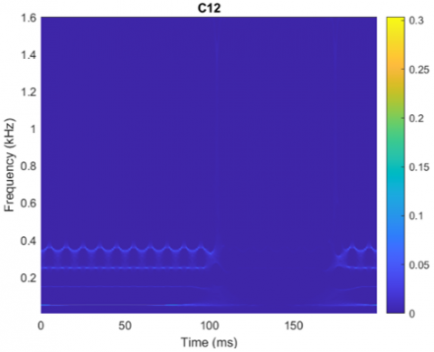
(a) Time-series signal
(b) WSST scheme
Figure 2. WSST scheme with the time-series signal of C12
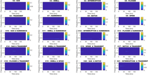
Figure 3. WSST schemes of time-series PQDs
$\begin{gathered}W_s(a, b)=\frac{1}{2 \pi} \int \hat{v}(\xi) a^{1 / 2} \overline{\hat{\psi}(a \xi)} e^{i b \xi} d \xi \\ W_s(a, b)=\frac{1}{i 4 \pi} \int[\delta(\xi-w)-\delta(\xi+w)] a^{1 / 2} \overline{\hat{\psi}(a \xi)} e^{i b \xi} d \xi\end{gathered}$ (5)
Wavelet $\psi$ is concentrated in positive frequency and so, FFT of, $\hat{\psi}(\xi)=0$ for $\xi<0$.
$W_s(a, b)=\frac{1}{i 4 \pi} a^{1 / 2} \overline{\hat{\psi}(a \xi)} e^{i b w}$ (6)
When $\overline{\hat{\psi}(a \xi)}$ is concentrated around $\xi=w_0, W_s(a, b)$ will be condensed around $a=w_0 / w$. By differentiating $W_s(a, b)$ with respect to $b$, the instantaneous frequency $w_{\text {inst }}(a, b)=2 \pi f_{\text {inst }}$ is obtained as:
$w_{\text {inst }}(a, b)=\frac{\frac{\partial W_s(a, b)}{\partial b}}{W_s(a, b)}$ (7)
It is supposed for a pure signal that $w_{\text {inst }}(a, b)=w(a, b)=w$. The time-scale plane is transferred to the time-frequency plane according to $(a, b) \rightarrow\left(b, w_{i n s t}(a, b)\right)$. For all the frequencies, concentrated CWT meaning WSST is obtained by the scaling with coefficient $a$ and the shifting with the instantaneous frequency, $w_{i n s t}$, for $W_s(a, b)$ which is given for the continuous time by Eq. (8)
$T_{\text {inst }}(w, b)=\int W_s(a, b) a^{-3 / 2} \delta\left(w_{\text {inst }}(a, b)-w\right) d a$ (8)
In this equation, the exponent of a can be changed to -1/2.
From 1D to the 2D conversion of the signal, i.e. from the time domain to the time-frequency domain, by using WSST for C12, one of the most complex problems, is shown with the time-series signal in Figure 2.
In this scheme, while harmonics are available in all timelines, sag emerges at 0.1 sec. and stops at 0.17 sec. While Figure 2(a). indicates the time domain information of the signal, Figure 2(b) shows frequency information as well as time. Hence, the time and frequency details of the signal can be analyzed easily. The WSST schemes of all PQDs excluding the C1 class of pure signal are given in Figure 3. In these schemes, light-colored lines with a heavy blue background are seen. From C6 to 21, intervals of disturbances can be seen explicitly because of the presence of variable character disturbances. The other disturbances, C2 to C5, have a smoother characteristic in which differences are observed when zoomed in. Although this situation seems like a disadvantage, both the amplitudes of the components leading to PQDs are condensed in a narrow band, and the unnecessary noise components are filtered. With these features, this method is more satisfactory than the classical methods like FFT, STFT, CWT, etc., as given in study [53]. For that reason, in this study, this method is selected to achieve higher classification performance.
The Eqs. (4) to (8) and Figure 2 show that the suggested WSST-based method is a good one that has a lot of potential. It is accurate, has a high level of resolution, and is robust when you look at the range of noise and the number of classes. Nevertheless, due to the nonlinear characteristics of the wavelets, the direct response of the WSST output is not available for each integer multiple of the frequency. Moreover, being a wavelet-based and 2D transformation method leads to computational load. In addition, this dataset is transmitted to CNN, which consists of a high-order matrix network. For all these reasons, one needs a higher-capacity computer or workstation than the other time- and time-frequency domain transformer-based hybrid models require.
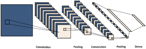
CNN is a human-brain-inspired neural network architecture. CNN is widely used in image recognition, segmentation, and classification fields due to its good performance. In CNN architecture, image recognition and classification, convolution, and pooling have an important role. Convolution and pooling are used for feature inference, size decrease, and the emphasis on important values, respectively. A basic CNN architecture consists of layers of convolution, pooling, and fully connected, which are shown in Figure 4.
Figure 4. A basic CNN structure
Convolutional Layer and Kernel
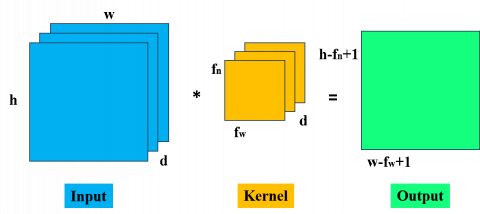
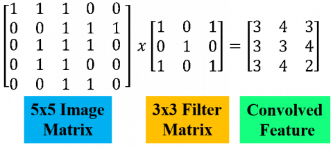
The convolutional layer is located at the core of the convolutional neural network, and convolutional operations are applied in this layer. The convolution operation is an operation that involves multiplying the input with a set of weights. A filter called the kernel is applied to the image to reduce its size by focusing on important locations in the image. In this layer, a filter with particular sizes is applied over the image, and the sum of the original pixel values is calculated by multiplying the weights specified in the filter. A convolved feature and its size are calculated by Eq. (9) based on the size of the input image and $f_h \times f_w \times d$ sized Kernel as shown in Figure 5.
$\left(h-f_h+1\right) \times\left(w-f_w+1\right)$ (9)
Padding
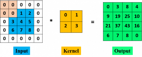
In CNNs, the presence of multiple convolution layers can result in the gradual shrinking of the original image, an undesirable outcome. Furthermore, the middle layer of the image undergoes more passes of the kernel compared to the edge layers, resulting in overlap. To address these issues, padding is introduced as an additional layer that can be appended to the image borders, preserving the original image's size. An application of padding to a (3×3) image with a kernel is illustrated in Figure 6. The size of the output image is obtained by Eq. (10) where p states the size of padding.
$\left(h-f_h+2 \mathrm{p}+1\right) \times\left(w-f_w+2 \mathrm{p}+1\right)$ (10)
Figure 5. Usage of kernel and obtaining convolved feature
Figure 6. Application of padding to (3x3) image
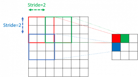
Strides
When the array is created, the pixels are shifted over to the input matrix. The number of pixels turning to the input matrix is known as the strides. When the number of strides is 2, the filters are carried to 2 pixels, as shown in Figure 7. Strides are responsible for regulating the features that could be missed while flattening the image. The size of an output image is calculated by Eq. (11).
Figure 7. Striding (2) with (3×3) filters on (7×7 image)
$\left(\frac{h-f_h+2 p}{s}+1\right) \times\left(\frac{w-f_w+2 \mathrm{p}}{s}+1\right)$ (11)
Pooling
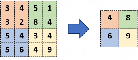
The pooling layers are generally seen between two convolution layers in CNN models. Pooling layers are used to decrease the size of the outputs from the convolution layer. Spatial pooling, also known as downsampling or subsampling, reduces the dimensionality of each map, the number of parameters, and computations in the network but retains the essential features, controlling overfitting by decreasing the size of the network. There are three types of spatial pooling: max, average, and sum pooling. The most commonly used one, max pooling, is a procedure that involves selecting the maximum value from a specified region, aiding in the extraction of the most vital features from an image, as illustrated in Figure 8. This process is sample-based and transforms continuous functions into discrete counterparts by downsizing the input.
Figure 8. Max pooling
The alternative pooling methods employed are analogous in approach but differ in their computational mechanisms; specifically, they calculate the average and sum of the values within the corresponding regions, respectively.
Flattening Layer
The task of this layer is simply to prepare the data at the input of the Fully Connected Layer. In general, neural networks receive input data from a one-dimensional array. The data in this neural network is the matrix coming from the convolutional and pooling layers converted into a one-dimensional array $\left(n \times n \rightarrow n^2 \times 1\right)$, as shown in Figure 9.
Figure 9. Flattening layer conversion
Fully-Connected Layer
The fully connected layer is the last and most important layer for CNN. It gets output from the last convolutional or pooling layer, which is flattened, gives the possibilities of each class, and performs the learning process. A scheme of the fully connected layer is given in Figure 10.
Figure 10. Fully-connected layer
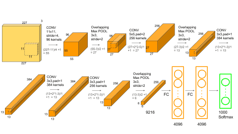
Figure 11. AlexNet architecture
For instance, one of the most known nets for image recognition is AlexNet. This is a CNN consisting of 8 layers, incorporating filters, stacked convolutional layers, max pooling, dropout, data augmentation, ReLU, and SGD, as shown in Figure 11 [56]. All resizements at each step were introduced in this figure. It comprises 5 convolution layers and 3 fully connected layers, totalling around 60 million parameters. However, a notable drawback of AlexNet is its reliance on a large number of hyperparameters.
Instead of a complex and time-consuming method, an efficient WSST-input CNN model is studied in this paper in order to detect and classify PQDs by researching in a narrowband hyperparameter space in the following section.
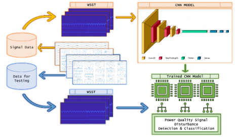
Comprehensive research for the proposed WSST and optimization of a CNN-based method for PQDs was done with a widespread space of CNN in this paper. All the processes carried out in this study are given as a scheme in Figure 12. In the beginning, the signal data is generated, and then the appointment of the zero-crossing points is carried out for the windowing process [8]. Later, 0.2-second (640-FFT)-windows are acquired with the help of these points. After these windowed signals are transformed with WSST, we obtain 2D signal packets. The best model of CNN with the related hyperparameters is selected on a workstation (with GPU: Nvidia Quadro P4000, CPU: Intel Xeon W-2223). At last, this model with the hyperparameters is able to detect and classify the PQDs. A similar zero-crossing process is performed to test the data. The best model and the related hyperparameters are processed to detect and classify PQD.
CNN models have been widely used in different engineering fields and, in recent years, have started to be used in power quality issues. CNN algorithms are preferred for classification data. The CNN model is used for classification purposes since the subject we discussed in this study is to describe the status and type of disturbances in power quality.
The data consists of 21 different classes. This data set has been processed with the WSST method, which has started to gain popularity today. The output of the data processing with the WSST method is taken as a 2D picture. These images were processed as RGB. The data are given as input data for the CNN model prepared after preprocessing.
The hyperparameter search space of the CNN model and the best CNN model obtained using this search space are delivered in Table 2.
As can be seen from the table, the research space is too large to calculate with the existing circumstances. For these reasons, a sketch CNN model as shown in Figure 13 without specific features and sizes of layers is exploited to obtain related hyperparameters. And then, the research space is restricted from general to private, considering the rules below.
All these rules narrow the research space, and research is applied. Then, the model with the highest accuracy rate is selected, as shown in Table 2.
The selected model is important in terms of accuracy and its low-number convolutional layers, despite high-size images such as 875×656. For the evaluation of performance, the accuracy rates of each research model are calculated and compared with each other.
Figure 12. Scheme of PQD detection and classification based on WSST & optimization of a CNN
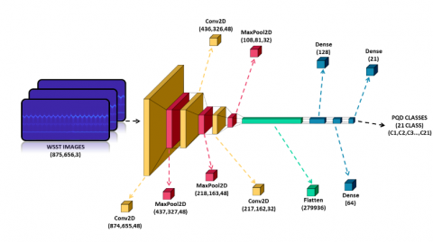
Figure 13. Proposed CNN structure for PQD classification
Table 2. Hyperparameter space of CNN and best CNN model
|
Hyperparameters Search Space |
|
|
Activations Functions |
['relu', 'sigmoid', 'selu', 'softplus', 'softsign', 'LeakyReLU', 'tanh', 'elu', 'exponential'] |
|
Optimizer |
['Adam', 'SGD', 'Adamax', 'Adadelta', 'Nesterov', 'Adagrad', 'RMSprop', 'Nadam', 'Ftrl'] |
|
Batch Size |
[10, 20, 32, 64, 128, 256, 512, 1024] |
|
Epoch |
[50,75,100,125,150,200] |
|
Learning Rate |
[0.0001, 0.0003, 0.0006, 0.001, 0.003, 0.006, 0.01, 0.03, 0.06] |
|
Layers |
[convolutional layer, dropout, pooling layer, dense, fully connected layer] |
|
Best CNN Model |
|
|
Activations Functions |
['linear', 'sigmoid'] |
|
Optimizer |
['Adam'] |
|
Batch Size |
[10] |
|
Epoch |
[100] |
|
Learning Rate |
[0.01] |
|
Layers |
['conv2d', 'max_pooling2d', 'conv2d_1', 'max_pooling2d_1', 'conv2d_2', 'max_pooling2d_2', 'flatten', 'dense', 'dense_1', 'dense_2'] |
|
Filters |
[48] |
|
Pool Size |
[3] |
|
Kernel Size |
[3] |
In this study, Tensorflow and Keras were used. TensorFlow is a library widely used for artificial intelligence tasks. In addition, Keras, an open-source library running on TensorFlow, was used. Keras was chosen for its overall ease of use, extensibility, and modularity.
6615 pre-processed images were given with a size of 875×656 in the type of RGB as input data to the selected CNN model. A total of 3 convolutions, 3 max-pooling, dense, and flattening layers are used in the model.
Figure 13 shows the summary of the proposed CNN structure. In the pooling process, max-pooling was chosen in the CNN model. Since the bright pixels in the WSST outputs are important in terms of frequency and location of the distortion, max-pooling was chosen to highlight these distinctive features in the picture. After the convolution and pooling processes, flattening was applied, and a dense layer was added. In the first and second of the last applied dense layers, the activation function was chosen as "linear." In the last layer, the sigmoid was applied as an activation function. Since there are 21 classes in the last layer, the last dense parameter is chosen as 21.
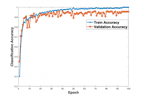
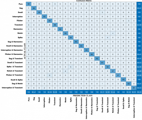
As stated before, primarily all time-series PQ datasets were converted to 2D by WSST. Then these 2D images have been run on a workstation to have the best CNN hyperparameters to use for the PQD classification. The numbers of training and validation are 1323 and 5282, with rationales of 20% and 80%, respectively. Also, test samples have the same ratio as validation samples. Figure 14 shows the training and validation accuracy versus the epoch of the model for 100 epochs. While train accuracy attains 0.9993 (converging to 1), validation accuracy converges to 0.9625. From the classification accuracy curves, there is a small difference between the test and validation samples. It can be indicated that the proposed model has good stability. In the proposed model, RGB figures are not resized as in the other studies, and with a high number of classes with noise and a low number of datasets, that’s why such a difference emerges between train and validation accuracy [35, 45, 57]. The confusion matrix in Figure 15 provides the results on the classification performance of PQD signals with the test dataset. The last rows and columns give the accuracy percent of actual and predicted values. The mean value of these accuracies is given as 96.25. The Figure 14 reveals that multiple disturbances have somewhat lower performance than singular disturbances because of their complex characteristics or the components of the multiple classes. Another notable thing is that singular or multiple disturbances with an oscillatory transient, C6, have some failings while others don’t. This is because the oscillatory transient is similar to the noise, too. Another erroneous detection belongs to singular or multiple disturbances for flicker because of a small frequency variation with this disturbance.
Table 3 shows the model accuracy rate of the proposed method in different SNR cases. As supposed, the accuracy rate increases with the SNR rate. But the results at the interval of 99.773% to 100% and the mean value of 99.93% In another way, the test accuracy results vary from 90.4% to 100% for 20 dB to 60 dB noise, and the mean value of the test results is 96.15%. These results are promising for PQDs when considering the number of classes, the noise range, and the low-number dataset.
Figure 14. Training and validation accuracies of the proposed model (achieved 0.9993 and 0.9625 respectively)
Figure 15. Confusion matrix
Table 3. The model accuracy rate for different SNRs
|
SNR |
Training Accuracy Rate |
Test Accuracy Rate |
|
20 |
99.773% |
90.476% |
|
30 |
99.924% |
93.936% |
|
40 |
99.924% |
97.070% |
|
50 |
100% |
99.244% |
|
60 |
100% |
100% |
|
Mean Value |
99.93% |
96.15% |
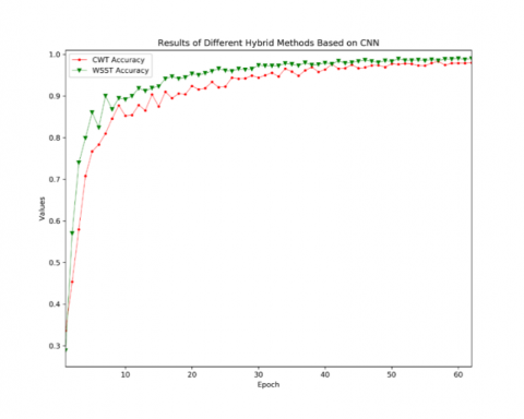
Comparative results are given in Figure 16 for CWT-CNN and the proposed method in terms of the accuracy curve. As can be seen, WSST has better performance than CWT, which is one of the most commonly used and effective methods in signal processing.
The proposed CNN-WSST-supported PQD D&C method is comparatively analyzed with similar methods under similar accuracy rates; the results are given in Table 4. This table indicates that when it accounted for all subparameters of the results, the proposed method had higher accuracy than the others, except for 1D-2D CNN [45] and Integrated Deep Learning [49], with an accuracy of 99.97% and 99.96%, respectively. Unlike the studies in Table 4, this study diversified the data with a high number of classes and a wide noise range, and thus the trained CNN model worked robustly. 21 classes were used in this study. In the data set, the noise range is set to 20-60 dB. This table indicates that, accounting for all subparameters of the results, the proposed method is more prosperous than the other methods, except for 1D-2D CNN [45] and IDL [49], with accuracies of 99.97% and 99.96%, respectively. Noticeably from Table 4, this study is one of the studies with the highest number of PQD classes and entirely randomly noisy data. The study performed in Sparse Signal Decomposition and Decision Tree [34] has better performance than this study with more PQD class variety but with a lesser noise range. Though the study performed in study [45] has more achievement than the proposed method in a wide noise range, it should be noticed that that study includes a smaller number of PQD classes. As compared with the studies in Table 4, in terms of accuracy, it is seen that only the study [45] has higher accuracy. But the proposed method is more comprehensive in terms of the number of PQD classes and the size of the noise range.
In this study, a hybrid method merges CNN and WSST, and optimization of it for PQD classification has been proposed for the first time. Apart from the other studies mentioned in Table 4, a comprehensive study based on WSST was conducted using CNN with a high PQD class number (21) and a dataset consisting of only noisy data (in the range of 20-60 dB). With this method, diversity and robustness have been provided, and results with higher accuracy have been obtained in comparison with the other studies, too.
Table 4. Comparative results of the proposed method
|
Method |
Class Number |
Noise Range |
Accuracy (%) |
||
|
Noisy (in…dB) |
Noiseless (in…dB) |
Mean |
|||
|
Hybrid Soft Computing - kNN & Support Vector Machines [12] |
10 |
- |
- |
98.75 |
98.75 |
|
Rule-Based Decision Tree & ST [24] |
6 |
20-50 |
98.1 (20) |
99.3 |
98.7 |
|
Fractional Fourier Transform [27] |
15 |
10-40 |
94.37 (20) |
99.93 |
97.2 |
|
ST Features [28] |
16 |
- |
- |
97.93 |
97.93 |
|
Volterra series with the Type-2 Fuzzy Logic System [29] |
6 |
20-30 |
98.83 (20) |
99.8 |
99.31 |
|
Strong Tracking Filters & Rule-based Extreme Learning Machine [30] |
20 |
20-40 |
92.6 (20) |
98.8 (40) |
95.7 |
|
HHT & kNN [31] |
18 |
20-30 |
97.38 (20) |
99 |
98.19 |
|
Linear KF & Fuzzy-Expert System [32] |
7 |
20-40 |
92.3 |
98.71 (40) |
95.5 |
|
Generalized Approach & KF [33] |
16 |
20-40 |
98.8 |
100 |
99.4 |
|
Sparse Signal Decomposition & Decision Tree [34] |
32 |
30-45 |
96.92 |
97.31 |
97.1 |
|
Multi-Objective Grey Wolf Optimizer, 2D-Riesz Transform, & kNN [35] |
18 |
20-40 |
99.56 (20) |
99.93 (40) |
99.75 |
|
Simple Gated Recurrent Network [37] |
15 |
- |
- |
99.07 |
99.07 |
|
Time-Dependent Spectral Featured & Adaptive kNN with Excluding Outliers [38] |
12 |
30-50 |
97.91 (30) |
99.81 |
98.86 |
|
Evolving Gaussian Fuzzy Classification [40] |
9 |
20-60 |
93.17 (60) |
- |
93.17 |
|
Variational Mode Decomposition & Detrended Fluctuation Analysis [41] |
9 |
10-30 |
99.38 (30) |
- |
99.38 |
|
DWT- Effective Feature Extraction |
10 |
- |
99.44 |
- |
99.44 |
|
Optimum Base Wavelet & MLA [43] |
14 |
20-50 |
93.29 (20) |
99.85 |
96.32 |
|
1D-2D CNN [45] |
13 |
0-50 |
- |
- |
99.97 |
|
Temporal Convolutional Network [46] |
8 |
- |
- |
99.82 |
99.82 |
|
Deep CNN [47] |
13 |
40-50 |
99.74 (50) |
99.61 |
99.67 |
|
Label-Guided Attention Method [48] |
7 |
20-50 |
99.30 (50) |
- |
99.20 |
|
Integrated DL [49] |
14 |
20-40 |
99.70 (20) |
99.98(40) |
99.96 |
|
Identification on DL [52] |
12 |
- |
- |
- |
99.70 |
|
Image-based Deep Transfer Learning [50] |
4 |
- |
- |
- |
99.3 |
|
Bagging LSTM [58] |
15 |
20-50 |
98.67 (20) |
99.66 (50) |
99,23 |
|
DL in 2D Scalogram [51] |
6 |
30-60 |
96.67 (30) |
97.33 (60) |
97,67 |
|
Proposed Method |
21 |
20-60 |
99.77 (20) |
100 (60) |
99.93 |
PQD signals are time-consuming due to their variational structure and are dangerous to obtain in the field. So, most studies are performed with experimental or only synthetic signals. While a synthetic one provides a wide range of signals and a high number of classes, experimental setups are more restricted in terms of types of equipment. In this study, a synthetic dataset generated in MATLAB for the training of the model is utilized, as mentioned before. Then, WSST is applied to all time signals. Finally, Python is utilized to build a CNN model with optimization through a training dataset, owing to the flexibility of Python in deep learning. Similarly, an experimental dataset is generated in an experimental setup for testing. The obtained dataset is processed with WSST in MATLAB. Eventually, the test dataset is performed on an optimized CNN model in Python for the evaluation of the proposed method. The experimental setup was established for the realization of the generation of the experimental dataset.
Figure 16. WT-based comparation of proposed method
This setup, consisting of an oscilloscope, two AATech 1032 Arbitrary Waveform Generators (AWG), a Rigol MSO 5204 Digital Storage Oscilloscope (DSO), a PC, 8 BNC connectors, and MATLAB and Python software, is used as figured out in Figure 17.
Initially, a 3.2 kHz (or more according to the specification of AWG) sampling frequency and 0.2 s window length providing a 5 Hz resolution are required in this setup, similar to some studies in studies [6-11]. In the first case of only one AWG usage, synchronization between AWGs and oscilloscopes was performed with a time-shifting arrangement. In the other case of two AWGs usage, both AWGs were tuned in phase, utilizing the AWGs’ consoles at first. Then, the obtained signals were arranged into the related window with the oscilloscope console, as in the first case. After the necessary preliminary preparations, AWGs are utilized to generate the signals based on variables and parameters with related intervals and scales in Table 1. These signals have time-varying noise, as illustrated in study [18], and therefore, noise addition is not required. BNC connectors transmit the signals to the DSO. After that, the transmitted signals are tuned into a 0.2-sec window. The whole signal at different channels is processed by different math functions to obtain the models in the table with the help of DSO's tool. As an example, the acquisition of a signal model is displayed in Figure 17(b) and clarified in the following paragraph, step by step. This method has been used for the generation of all event classes. The obtained 0.2-second signals are compiled in MATLAB and applied to signal processing with WSST on PC. After that, WSST images are used for testing on the optimized CNN model in Python.
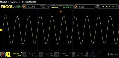
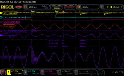
C1 class, a pure signal, is seen having about 36 dB of spontaneous grid noise on the DSO monitor in Figure 18(a). While single classes like 5, 8, and 9 can be generated by only an AWG, lots of them need at least two AWGs and 8 BNC probes. One of the multiple disturbance events, C14, comprising the sag and transient signals, is given with all subcomponents in Figure 18(b). For the generation of this signal,
(a) An image from the setup
(b) Flowchart of the test setup
Figure 17. PQD event generation to test proposed model
(a) C1
(b) C14
Figure 18. PQD events from the DSO’s monitor for different classes
All PQD classes are generated with about 36 dB of spontaneous grid noise under the mathematical models from AWG, as seen in the comprehensive waveforms in Figure 18(a). Further, since two different AWGs are needed, a phase shift is formed that must be coped with. Taking into account all these circumstances, it is seen that the generated signals to test the proposed model are disturbed, which is similar to field data. Herewith, the experimental dataset is obtained by this method.
This investigation has led to the development of a method that integrates WSST with an optimized CNN for the detection and classification of a wide array of PQDs in environments characterized by noise and rapid signal variation. A comparative analysis of several CNN models was conducted, focusing on accuracy metrics. Subsequently, the most efficacious model was selected through an optimization process. The application of WSST-enhanced images for PQD classification with this optimized CNN model is a novel approach undertaken in this study. It yielded notable accuracy rates, achieving 99.93% in training and 96.15% in testing scenarios, despite the challenges posed by a diverse range of classes and noise levels. The robustness of this method in the face of signal noise and variation is crucial for accurate PQD analysis. Results have demonstrated that this robust approach maintains high accuracy across datasets characterized by significant class and noise diversity. Furthermore, the classification accuracy of PQDs has been enhanced, alongside a simplification in computation. Within the constraints of the available hardware, a dataset comprising 6615 time-series signals, encapsulating 21 PQD classes across noise intervals of 20 dB to 60 dB, was transformed using WSST. Subsequent training and testing were executed on a medium-capacity workstation. Future research could extend the dataset size and the number of classes, contingent on the availability of more advanced computational resources and experimental setups. Overcoming these hardware limitations could pave the way for more expansive datasets, fostering the development of comprehensive, stable, and robust methods.
Thanks to Sivas University of Science and Technology for providing the experimental setup.
[1] "IEEE Recommended Practice for Monitoring Electric Power Quality," in IEEE Std 1159-1995, pp. 1-80, 30 Nov. 1995, https://doi.org/10.1109/IEEESTD.1995.79050
[2] "IEEE Standard Definitions for the Measurement of Electric Power Quantities Under Sinusoidal, Nonsinusoidal, Balanced, or Unbalanced Conditions," in IEEE Std 1459-2010 (Revision of IEEE Std 1459-2000), pp. 1-50, 19 March 2010. https://doi.org/10.1109/IEEESTD.2010.5439063
[3] Standard, I., Internationale, N. (2008). IEC standard 61000-4-7: General guide on harmonics and interharmonics measurements and instruments for power supply networks and attached devices used for the measurements.
[4] "IEEE Recommended Practice--Adoption of IEC 61000-4-15:2010, Electromagnetic compatibility (EMC)--Testing and measurement techniques--Flickermeter--Functional and design specifications," in IEEE Std 1453-2011, pp. 1-58, 21 Oct. 2011. https://doi.org/10.1109/IEEESTD.2011.6053977
[5] International Electrotechnical Commission. (2003). IEC standard 61000-4-30: Testing and measurement techniques - Power quality measurement methods (IEC 61000-4-30 ed.).
[6] Akkaya, S., Salor, Ö. (2022). Flicker detection algorithm based on the whole voltage frequency spectrum for new generation lamps – Enhanced VPD flickermeter model and flicker curve. Electric Power Components Systems, 1-15. https://doi.org/10.1080/15325008.2021.2011487
[7] Akkaya, S., Salor, Ö. (2018). A new flicker detection method for new generation lamps both robust to fundamental frequency deviation and based on the whole voltage frequency spectrum. Electronics (Switzerland), 7(6): 99. https://doi.org/10.3390/electronics7060099
[8] Akkaya, S., Salor Durna, Ö. (2018). Enhanced spectral decomposition method for light flicker evaluation of incandescent lamps caused by electric arc furnaces. Journal the Faculty of Engineering and Architecture of Gazi University, 2018(18-2): 987-1005. https://doi.org/10.17341/gazimmfd.460497
[9] Akkaya, S., Salor, Ö. (2019). New flickermeter sensitive to high-frequency interharmonics and robust to fundamental frequency deviations of the power system. IET Science, Measurement and Technology, 13(6): 735-742. https://doi.org/10.1049/iet-smt.2018.5338
[10] Gençol, K. (2021). Choosing the optimum frequency estimator under system frequency deviations in power systems. European Journal of Science and Technology, 27: 670-675. https://doi.org/10.31590/ejosat.904157
[11] Khoa, N.M., Van Dai, L. (2020). Detection and classification of power quality disturbances in power system using modified-combination between the stockwell transform and decision tree methods. Energies (Basel), 13(14): 3623. https://doi.org/10.3390/en13143623
[12] Manimala, K., Selvi, K., Ahila, R. (2011). Hybrid soft computing techniques for feature selection and parameter optimization in power quality data mining. Applied Soft Computing Journal, 11(8): 5485-5497. https://doi.org/10.1016/j.asoc.2011.05.010
[13] Verma, A.K., Jarial, R.K., Roncero-Sanchez, P., Ungarala, M.R. (2021). Improved fundamental frequency estimator for three-phase application. IEEE Transactions on Industrial Electronics, 68(9): 992-898. https://doi.org/10.1109/TIE.2020.301063
[14] Crotti, G., D’Avanzo, G., Letizia, P.S., Luiso, M. (2021). Measuring harmonics with inductive voltage transformers in presence of subharmonics. IEEE Transactions on Instrumentation and Measurement, 70: 1-13. https://doi.org/10.1109/TIM.2021.3111995
[15] Kuwalek, P., Wiczynski, G. (2021). Dependence of voltage fluctuation severity on clipped sinewave distortion of voltage. IEEE Transactions on Instrumentation and Measurement, 70: 1-8. https://doi.org/10.1109/TIM.2021.3102693
[16] Lv, J. (2022). Transient stability assessment in large-scale power systems using sparse logistic classifiers. International Journal of Electrical Power and Energy Systems, 136: 107626. https://doi.org/10.1016/j.ijepes.2021.107626
[17] Santos, C.H.T., Pereira, V (2022). Envelope estimation using geometric properties of a discrete real signal. Digital Signal Processing: A Review Journal, 120: 103229. https://doi.org/10.1016/j.dsp.2021.103229
[18] Akkaya, S., Yüksek, E., Akgün, H.M. (2023). A new comparative approach based on features of subcomponents and machine learning algorithms to detect and classify power quality disturbances. Electric Power Components and Systems, 1-24. https://doi.org/10.1080/15325008.2023.2260375
[19] Xi, Y., Li, Z., Zeng, X., Tang, X., Liu, Q., Xiao, H. (2018). Detection of power quality disturbances using an adaptive process noise covariance Kalman filter. Digital Signal Processing: A Review Journal, 76: 34-49. https://doi.org/10.1016/j.dsp.2018.01.013
[20] Ndoumbe, L.D., Eke, S., Kom, C.H., Yeremou, A.T., Nanfak, A., Ngaleu, G.M. (2021). Power quality problems, signature method for voltage dips and swells detection, classification and characterization. European Journal of Electrical Engineering, 23(3): 185-195. https://doi.org/10.18280/ejee.230303
[21] Xiao, F., Lu, T., Wu, M., Ai, Q. (2020). Maximal overlap discrete wavelet transform and deep learning for robust denoising and detection of power quality disturbance. IET Generation, Transmission & Distribution, 14(1): 140-147. https://doi.org/10.1049/iet-gtd.2019.1121
[22] Tiwari, V.K., Umarikar, A.C., Jain, T. (2020). Measurement of instantaneous power quality parameters using UWPT and Hilbert transform and its FPGA implementation. IEEE Transactions on Instrumentation and Measurement, 70: 1-13. https://doi.org/10.1109/TIM.2020.3021769
[23] Yu, Y., Zhao, W., Li, S., Huang, S. (2021). A two-stage wavelet decomposition method for instantaneous power quality indices estimation considering interharmonics and transient disturbances. IEEE Transactions on Instrumentation and Measurement, 70: 1-13. https://doi.org/10.1109/TIM.2021.3052554
[24] Zaro, F. (2021). Power quality disturbances detection and classification rule-based decision tree. International Journal of Engineering Science and Application, 5(1): 1-6. https://doi.org/10.37394/232014.2021.17.3
[25] Reddy, M.J(b), Raghupathy, R.K., Venkatesh, K.P., Mohanta, D.K. (2013). Power quality analysis using Discrete Orthogonal S-transform (DOST). Digital Signal Processing, 23(2): 616-626. https://doi.org/10.1016/j.dsp.2012.09.0
[26] Singh, U., Singh, S.N. (2017). Detection and classification of power quality disturbances based on time-frequency-scale transform. IET Science, Measurement and Technology, 11(6): 802-810. https://doi.org/10.1049/iet-smt.2016.0395
[27] Singh, U., Singh, S.N. (2017). Application of fractional Fourier transform for classification of power quality disturbances. IET Science, Measurement and Technology, 11(1): 67-76. https://doi.org/10.1049/iet-smt.2016.0194
[28] Pandya, V., Agarwal, S., Mahela, O.P., Choudhary, S. (2020). Detection and classification of complex power quality disturbances using hybrid algorithm based on combined features of Stockwell transform and Hilbert transform. In 2020 IEEE International Students’ Conference on Electrical, Electronics and Computer Science (SCEECS), Bhopal, India, pp. 1-6. https://doi.org/10.1109/SCEECS48394.2020.4
[29] Kapoor, R., Kumar, R., Tripathi, M.M. (2018). Volterra bound interval type-2 fuzzy logic based approach for multiple power quality events analysis. IET Electrical Systems in Transportation, 8(3): 188-196. https://doi.org/10.1049/iet-est.2017.0054
[30] Chen, X., Li, K., Xiao, J. (2018). Classification of power quality disturbances using dual strong tracking filters and rule-based extreme learning machine. International Transactions on Electrical Energy Systems, 28(7): e2560. https://doi.org/10.1002/etep.2560
[31] Mishra, M. (2019). Power quality disturbance detection and classification using signal processing and soft computing techniques: A comprehensive review. International Transactions on Electrical Energy Systems, 29(8): e12008. https://doi.org/10.1002/2050-7038.12008
[32] Abdelsalam, A.A., Eldesouky, A.A., Sallam, A.A. (2012). Classification of power system disturbances using linear Kalman filter and fuzzy-expert system. International Journal of Electrical Power and Energy Systems, 43(1): 688-695. https://doi.org/10.1016/j.ijepes.2012.05.052
[33] Abdelsalam, A.A., Abdelaziz, A.Y., Kamh, M.Z. (2021). A generalized approach for power quality disturbances recognition based on Kalman filter. IEEE Access, 9: 93614-93628. https://doi.org/10.1109/ACCESS.2021.3093367
[34] Manikandan, M.S., Samantaray, S.R., Kamwa, I. (2015). Detection and classification of power quality disturbances using sparse signal decomposition on hybrid dictionaries. IEEE Transactions on Instrumentation and Measurement, 64(1): 27-38. https://doi.org/10.1109/TIM.2014.2330493
[35] Karasu, S., Saraç, Z. (2020). Classification of power quality disturbances by 2D-Riesz Transform, multi-objective grey wolf optimizer and machine learning methods. Digital Signal Processing: Review Journal, 101: 102711. https://doi.org/10.1016/j.dsp.2020.102711
[36] Narayanaswami, R., Sundaresan, D., Prema, V.R. (2021). The mystery curve: A signal processing based power quality disturbance detection. IEEE Transactions on Industrial Electronics, 68(10): 10078-10086. https://doi.org/10.1109/TIE.2020.3026268
[37] Zu, X., Wei, K. (2021). A simple gated recurrent network for detection of power quality disturbances. IET Generation, Transmission and Distribution, 15(4): 751-761. https://doi.org/10.1049/gtd2.12056
[38] Liu, Y., Jin, T., Mohamed, M.A., Wang, Q. (2021). A novel three-step classification approach based on time-dependent spectral features for complex power quality disturbances. IEEE Transactions on Instrumentation and Measurement, 70: 1-14. https://doi.org/10.1109/TIM.2021.3050187
[39] Altay, T., Baydoğan, M.G. (2021). A new feature-based time series classification method by using scale-space extrema. Engineering Science and Technology, an International Journal, 24: 1490-1497. https://doi.org/10.1016/j.jestch.2021.03.017
[40] Leite, D., Decker, L., Santana, M., Souza, P. (2020). EGFC: Evolving gaussian fuzzy classifier from never-ending semi-supervised data streams - with application to power quality disturbance detection and classification. In 2020 IEEE International Conference on Fuzzy Systems, Glasgow, UK, pp. 1-9. https://doi.org/10.1109/FUZZ48607.2020.9177847
[41] Xu, Y., Gao, Y., Li, Z., Lu, M. (2020). Detection and classification of power quality disturbances distribution networks based on VMD and DFA. CSEE Journal of Power and Energy Systems, 6(1): 122-130. https://doi.org/10.17775/CSEEJPES.2018.01340
[42] Khetarpal, P., Tripathi, M.M. (2020). A critical and comprehensive review on power quality disturbance detection and classification. Sustainable Computing: Informatics and Systems, 28: 100417. https://doi.org/10.1016/j.suscom.2020.100417
[43] Meena, H., Meena, H.K., Saxena, D. (2022). Classification of power quality disturbances with DWT based effective feature extraction. In 2021 4th International Conference on Recent Trends in Computer Science and Technology (ICRTCST), Jamshedpur, India, pp. 314-320. https://doi.org/10.1109/ICRTCST54752.2022.9781895
[44] Hafiz, F., Swain, A., Naik, C., Abecrombie, S., Eaton, A. (2019). Identification of power quality events: Selection of optimum base wavelet and machine learning algorithm. IET Science, Measurement and Technology, 13(2): 260-271. https://doi.org/10.1049/iet-smt.2018.5044.
[45] Sindi, H., Nour, M., Rawa, M., Öztürk, Ş., Polat, K. (2021). A novel hybrid deep learning approach including combination of 1D power signals and 2D signal images for power quality disturbance classification. Expert Systems with Applications, 174: 114785. https://doi.org/10.1016/j.eswa.2021.114785
[46] Yang, Z., Liao, W., Liu, K., Chen, X., Zhu, R. (2022). Power quality disturbances classification using a TCN-CNN model. In 2022 IEEE Applied Power Electronics Conference and Exposition (APEC), Hangzhou, China, pp. 2145-2149. https://doi.org/10.1109/acpee53904.2022.9783716
[47] Xue, H., Chen, A., Zhang, D., Zhang, C. (2020). A novel deep convolution neural network and spectrogram based microgrid power quality disturbances classification method. In 2020 IEEE Applied Power Electronics Conference and Exposition (APEC), New Orleans, LA, USA, pp. 2303-2307. https://doi.org/10.1109/APEC39645.2020.9124252
[48] Gu, D., Gao, Y., Li, Y., Zhu, Y., Wu, C. (2021). A novel label-guided attention method for multilabel classification of multiple power quality disturbances. IEEE Transactions on Industrial Informatics, 18(7): 4698-4706. https://doi.org/10.1109/TII.2021.3115567
[49] Xiao, X., Li, K. (2021). Multi-Label Classification for Power Disturbances by Integrated Deep Learning. IEEE Access, 9: 152250-152260. https://doi.org/10.1109/ACCESS.2021.3124511
[50] Todeschini, G., Kheta, K., Giannetti, C. (2022). An image-based deep transfer learning approach to classify power quality disturbances. Electric Power Systems Research, 213: 108795. https://doi.org/10.1016/j.epsr.2022.108795
[51] Salles, R.S., Ribeiro, P.F. (2023). The use of deep learning and 2-D wavelet scalograms for power quality disturbances classification. Electric Power Systems Research, 214: 108834. https://doi.org/10.1016/j.epsr.2022.108834
[52] Wang, N., Sun, M., Xi, X. (2024). Identification of power quality disturbance characteristic based on deep learning. Electric Power Systems Research, 226: 109897. https://doi.org/10.1016/j.epsr.2023.109897
[53] Akan, A., Karabiber, C. (2021). Time-frequency signal processing: Today and future. Digital Signal Processing: A Review Journal, 1(1): 103216. https://doi.org/10.1016/j.dsp.2021.103216
[54] Daubechies, I., Lu, J., Wu, H.T. (2011). Synchrosqueezed wavelet transforms: An empirical mode decomposition-like tool. Applied and Computational Harmonic Analysis, 30(2): 243-261. https://doi.org/10.1016/j.acha.2010.08.002
[55] Thakur, G., Brevdo, E., Fučkar, N.S., Wu, H.T. (2013). The Synchrosqueezing algorithm for time-varying spectral analysis: Robustness properties and new paleoclimate applications. Signal Processing, 93(5): 1079-1094. https://doi.org/10.1016/j.sigpro.2012.11.029
[56] Nayak, S. (2023). UnderstandingNet. Retrieved November 14, 2023, from https://learnopencv.com/understanding-alexnet/
[57] Tang, S., Zhu, Y., Yuan, S. (2022). Intelligent fault identification of hydraulic pump using deep adaptive normalized CNN and synchrosqueezed wavelet transform. Reliability Engineering & System Safety, 224: 108560. https://doi.org/10.1016/j.ress.2022.108560
[58] Wang, J., Zhang, D., Zhou, Y. (2022). Ensemble deep learning for automated classification of power quality disturbances signals. Electric Power Systems Research, 213: 108695. https://doi.org/10.1016/j.epsr.2022.108695