Ranjith Subramanian*![]() | Jesu Jayarin
| Jesu Jayarin![]() | Arumugam Chandrasekar
| Arumugam Chandrasekar![]()
© 2023 IIETA. This article is published by IIETA and is licensed under the CC BY 4.0 license (http://creativecommons.org/licenses/by/4.0/).
OPEN ACCESS
Future 6G wireless networks are anticipated to support a variety of gadgets, including smartphones, tablets, smart home sensors, etc. One of the most significant problems that limits the operation of wireless networks as the number of connected devices rises is interference. With the advent of 6G wireless networks, new use cases and applications are emerging that adhere to tight standards for next-generation wireless communications. On TV, radio, or mobile phones, interference causes poor reception of the images or sounds. EM (Electromagnetic) waves are used as the transport medium in these communication systems. Therefore, recent research has focused on the potential of DL techniques in fulfilling these stringent requirements and addressing the drawbacks of existing model-based methodologies. In 6G MIMO channel estimation with interference alignment, this research proposes a unique method based on a heterogeneous network and deep learning methods. HetNet-based multiuser propagation is used in this case to estimate the channel. A hybrid transfer convolutional network has been used to align the network's interference. We design an Orthogonal Frequency Division Multiplexing (OFDM) frame structure to illustrate the allocation of time-frequency resources to pilot signals for channel estimation. It is important to note that the proposed framework does not require information transmission between BSs and instead operates in a non-iterative and distributed manner based on local channel state information (CSI) at both BSs and users.
6G MIMO, channel estimation, interference alignment, heterogeneous network, deep learning, OFDM, resource allocation
The massive use of wireless devices on daily basis requires a new generation (6G) of wireless communications that can provide aggregate date rates of Tb/s per access point. Furthermore, these new wireless networks must introduce features such as high achievable data rates, low latency, low power consumption, security, and high reliability. Therefore, new methods are needed in 6G to achieve these objectives including high data rate transceivers, new network architectures and efficient interference management schemes [1]. In both industrial and academic communities, optical wireless communication (OWC) is increasingly being considered as a promising technology that can support the escalating user demands where the optical spectrum provides a huge and license-free bandwidth, satisfying part of the requirements of 6G networks. visible light communication (VLC) using light emitting diodes (LEDs) is deployed for providing illumination as well as communication. It is shown that VLC can outperform traditional radio frequency (RF) wireless networks in terms of achievable data rates and aggregate capacity. It is worth mentioning that there are currently significant standardization efforts for OWC in the 802.11bb standard and its integration in the Internet protocol (IP) network, usually referred to as Light-Fidelity (LiFi) [2]. However, using LEDs for data transmission limits the performance of OWC systems where these sources have a limited modulation speed.
The wireless industry has been encouraged to take into consideration mmW for Fifth Generation of cellular networks (5G), as well as Vehicle-to-Everything (V2X) applications due to recent advancements in millimeter-wave (mmW) hardware as well as probable availability of spectrum [3]. Sub-THz systems for 6G networks are anticipated, continuing the same trend [4]. This results in highly sparse channels. Several Input A saving grace is the use of Multiple Output Multiple Input (MIMO) systems, which can offer a beamforming gain to get around route loss as well as build links with a respectable Signal-to-Noise Ratio (SNR). Precoding and stream combining are made possible by MIMO systems, which could greatly increase the potential data rate. The hardware in mmW/sub-THz band is subject to a number of non-trivial practical restrictions, despite fact that fundamental principle of MIMO precoding/combining is same regardless of carrier frequency [5]. In conventional MIMO systems, processing is carried out digitally at baseband, necessitating a separate RF chain for every antenna element. This indicates a significant cost as well as power consumption due to large number of elements needed in mmW, rendering it impractical. First, Hybrid Beamforming (HBF) was presented and examined. It is motivated by the notion that, if suitable precoding/combining is used, the number of antenna elements will determine beamforming gain as well as diversity. In order to achieve analogue precoding/combining, phase shifters, switches, or lenses are frequently used. The components of the RF precoder are subject to the restriction of constant amplitude imposed by an HBF based on a phase shifting network [6].
Research contribution are as follows: In MIMO interference networks with fixed channel coefficients and no symbol extensions, we discuss the viability of linear IA. The conclusions presented here do not hold if multiple channel uses are taken into account; instead, they are focused on the recently popular single channel use IA feasibility problem. The solution to a set of polynomial equations and some partial findings constitute this issue. The major contribution of this study, which is a straightforward feasibility test that essentially checks the rank of a certain matrix, may be derived from this finding. We offer precise arithmetic and floating-point variants of the test, together with a thorough complexity analysis that demonstrates the problem's impossibility for general MIMO channels. The primary contribution is given below:
(1) To propose novel method in 6G MIMO channel estimation with interference alignment based on heterogeneous network with deep learning techniques;
(2) To develop channel estimation model using HetNet based multiuser propagation model;
(3) To design interference alignment model using hybrid transfer convolutional network.
Theoretical analyses of IA have been done in a number of studies. Degrees of Freedom (DoF) is a common statistic used to describe IA. The amount of space that is devoid of interference is referred to as the DoF [7]. Examples are given by Wang et al. [8] to illustrate how IA and varying DoF can be achieved in K-User interference networks with various antenna designs. For a TDD mode of operation, an iterative approach for producing precoders as well as beamformers is provided by Pan et al. [9]. The bidirectional relationship between MIMO forward as well as reverse channels determines how the precoders work in this manner. Nasser et al. [10] presents yet another IA framework using TDD channels. Xu et al. [11] investigates interference alignment in MIMO downlink networks where precoders are created through eigen decomposition of MIMO channels. Ren et al. [12] makes a new IA proposal for a K-User MIMO X network. This approach maximises the amount of interference-free space by reducing interference at each mobile device to half of the received signal space by suitably precoding the broadcast signals. Furthermore, interference cancellation for K=3 has been accomplished by using a zero forcing beamformer that is a function of interfering channels as well as precoders. The methods in Fanjul et al. [13] are entirely theoretical, and we develop on them in this study. There is no explanation on how to demodulate symbols. Additionally, we want to operate K-User MIMO X method so that every access point transmits various symbols to every mobile device while operating on same frequency subcarrier in order to maximise capacity. We looked into the scenario where every access point is on a various subcarrier in Mafuta and Walingo [14] as well as discovered that there is a considerable reduction in bandwidth as well as consequently capacity of K-User method by a factor of K. A multi-cell cooperative downlink channel was initially researched in Ranjith et al. [15]. The authors used dirty paper coding (DPC) to create the perfect backhaul network with one antenna for every user as well as BS. Benaya and Elsabrouty [16] investigated BS cooperation for MIMO to reduce co-channel interference using cooperative transmission techniques. In Wang et al. [17], an iterative technique was suggested to optimise beamforming vector as well as power allocations based on an uplink-downlink duality property. In Qamar et al. [18], an effective iterative technique based on uplink-downlink duality and Lagrangian theory was presented for coordinated beamforming vectors across all BSs in decentralised multi-cell downlink. Additionally, based on the primal-dual optimality theory, a novel transmits precoding method for multiple access spatial modulation MIMO was presented in Suo et al. [19]. Through the use of super-resolution technology, a DL based low overhead analogue beam selection technique was created in Muta et al. [20], as well as beam quality prediction method was created. When MRC as well as random choice of LSFD, which were introduced in Liu et al. [21], were utilized in first as well as second decoding layers, closed form of uplink SE was derived for correlated Rayleigh fading environment. For MIMO system based on DL, numerous channel estimation algorithms have been established in the Ali et al. [22]. However, the channel plans were approximated without taking the obtained SNR feedback into account. For the MIMO system, a number of channel modelling strategies have been proposed in Najlah, and Sameer [23]. Additionally, for the massive MIMO system, DL -based direction-of-arrival (DOA) estimate method as well as hybrid precoding methods are proposed in Rajoria et al. [24]. Methods of Mellempudi and Pamula [25] however, presuppose some particular channel methods are parameterized by a number of variables, including array response, angle-of-departure, and direction-of-arrival.
Uncoordinated interference, which significantly reduces the performance of the coordinated part of the network, is a significant problem for IA approaches. For instance, in heterogeneous pico-cell networks, interference from femto and home base stations is frequently an uncoordinated source, and the users who are connected to them aren't always able to collaborate. As a result, their interference cannot completely align. Furthermore, interference is a serious problem for relay-aided MIMO networks since it simultaneously affects the signal received at the relay and the destination. Relay processing matrix design also becomes a challenging problem. Unfortunately, because the power limits of relays depend on the precoding matrices at transmitters as well as the processing matrices at the relays, earlier single-hop IA techniques are not easily adaptable to relay-aided situations.
2.1 Problem formulation
Vectorizing the received signal matrix Y is important to take advantage of the MIMO channel's sparseness (1). After denoting $\frac{\operatorname{vec}(\mathbf{Y})}{\sqrt{P_p}}$ by $\mathbf{y} \in \mathbb{C}^{N_t^{\text {beam }} N_r^{\text {beam }} \times 1}$ we have:
$Y=\left(\left(F_D^T F_R^T\right) \otimes\left(W_D^H W_R^H\right)\right) {vec}(H)+z={ }^{(b)}Qvec(G)+z$ (1)
Equivalent noise vector $z \triangleq \frac{1}{\sqrt{P}}\left[\mathbf{z}_1^T, \cdots, \mathbf{z}_{N_t^{\text {bosm }}}^T\right]^T \in \mathbb{C}^{N_t^{\text {hesam }} N_r^{\text {hesm }} \times 1}$ and properties of Kronecker product, $\operatorname{vec}(\mathbf{A B C})=\left(\mathbf{C}^T \otimes \mathbf{A}\right) \operatorname{vec} (\mathbf{B})$ and $(\mathbf{A} \otimes \mathbf{B})^T=\mathbf{A}^T \otimes \mathbf{B}^T$, and (b) follows from $\operatorname{vec}(\mathbf{H})=\left(\mathbf{A}_i^* \otimes \mathbf{A}_r\right) \operatorname{vec}(\mathbf{G})$ and $(\mathbf{A} \otimes \mathbf{B})(\mathbf{C} \otimes \mathbf{D})=(\mathbf{A C}) \otimes(\mathbf{B D})$. Equivalent sensing matrix $\mathrm{Q} \in \mathbb{C}^{N_t^{\text {besm }}} N_{+}^{\text {thesm }} \times N_t^{\text {iot }} N_{+}^{\text {tot }}$ are described as Eq. (2):
$Q \triangleq\left(F_D^T F_R^T A_t^*\right) \otimes\left(W_D^H W_R^H A_r\right)$ (2)
Since vec (G) only has $N_0=\left|\Omega_c\right|+\sum_{m=1}^{M_r} \sum_{n=1}^{M_t}\left|\Omega_{m, n}^1\right|$ non-zero elements and $\dot{N}_0 \ll N_t^{\mathrm{tot}} N_r^{t \text { tot }}$, the formulation of vectorized received signal in (2) gives a sparse formulation of channel estimation issue. This suggests that number of observations needed to find non-zero elements, $N_t^{\text {beam }} N_r^{\text {beam }}$ may be considerably lower $N_t^{\text {tot }} N_r^{\text {tot }}$. To decrease amount of training needed and enhance channel estimation performance, we plan to take use of the hidden joint sparsity in beam-domain channel. To create a new vector with a block of equal length for MtMr, we simply reverse order of the items in vec (G) Eq. (3):
$\mathbf{x} \triangleq\left[\mathbf{x}_1^T, \cdots, \mathbf{x}_{M M_t M_r}^T\right]^T=[\underbrace{\operatorname{vec}^T\left(\mathbf{G}_{1,1}\right)}_{\text {1th block }}, \cdots, \underbrace{\operatorname{vec}^T\left(\mathbf{G}_{M_r, 1}\right)}_{M_r \text { th block }} \underbrace{\operatorname{vec}^T\left(\mathbf{G}_{1, M_t}\right)}_{\left(M_r\left(M_t-1\right)+1\right) \text { th block }}, \cdots, \underbrace{\operatorname{vec}^T\left(\mathbf{G}_{M_r, M_t}\right)}_{M_t M_r \text { th block }}]^T$ (3)
where, block size is $N_t^{\text {sub }} N_r^{\text {sub }}$ By switching the column order of $\Phi \triangleq \mathbf{Q} \Pi \Phi$, where is a column permutation matrix, so that $\Phi \mathbf{x}=\mathbf{{Qvec}}(\mathbf{G})$, corresponding equivalent measurement matrix Q is (G). Issue of MIMO channel recovery at RX can therefore be expressed as Eq. (4):
$\min _{\times}\|\mathbf{y}-\boldsymbol{\Phi} \mathbf{x}\|_2^2$ (4)
Due to frequent as well as innovative sparsity requirements in constraint, which are considerably varied from traditional CS-recovery issue with a basic sparsity (l0-norm) constraint, issue (4) is exceedingly difficult. Additionally, equivalent measurement matrix needs to be carefully planned in order to ensure non-zero members of vector may be recovered with a high degree of probability while only requiring a few measurements.
We'll take into account a MIMO method with a transmitter as well as receiver. Mt antennas are used in the transmitter, and Mr antennas are used in the receiver. At every symbol time, transmitter provides pilot symbols that the reception already knows about for purpose of channel estimation. The receiver then feeds back to transmitter received SNR values that were calculated at its antennas. Each symbol time is believed to have a number of mini-time slots, first Np consecutive mini-time slots of which are reserved for transmission of pilot symbols. Received signal at receiver is given by Eq. (5) at nth symbol time.
$R(n)=H(n) S(n)+Q(n)$ (5)
where, $Q(n) \in C^{M_F \times N_p}$ is matrix of received noises. Also, $S(n) \triangleq\left[s_1(n), \cdots, s_{N_F}(n)\right] \in C^{M_4 \times N_p}$ is matrix of pilot symbols, where $s_m(n) \in C^{M x 1}$ is vector of pilot symbols. The pilot symbol matrix S shall simply be referred to as pilot signal in this article. $\|S\|_F^2=\operatorname{Tr}\left(S S^H\right) \leq P$ , where P stands for maximum transmit power at transmitter, limits transmit power of pilot signal.
By vectorizing R(n) of (1) and utilizing result of ${vec}(A X B)=\left(B^T \otimes A\right) {vec}(X)$ we have by Eq. (6):
$r(n)=\left(S^T(n) \otimes I_{M_*}\right) h(n)+q(n)$ (6)
where, $s_1(n), \cdots, s_{N_F}(n)$. The elements of $\left.g(n)\left|\left(S^T(n) \otimes I_{M_r}\right) h(n)\right|\right)$ and h(n) is variance of every element of q, give received SNR (or SSI/CQI) values calculated at antennas of receiver during pilot signal transmission (n). In this study, it is presumed that the transmitter only receives the magnitudes of received SNR values elements of $\left.g(n)\left|\left(S^T(n) \otimes I_{M_r}\right) h(n)\right|\right)$. As a result, at nth symbol time, Eq. (7) provides feedback signal that transmitter has received.
$\left.\gamma(n)=g(n)\left|\left(S^T(n) \otimes I_{M_r}\right) h(n)\right|\right)$ (7)
where, η(n) is noise-plus-error component of SNR feedback, which accounts for limitations of SNR estimate, measurement, quantization, etc.
3.1 Channel estimation
To acquire the best precoder design, it is critical to evaluate channel with high accuracy because it is a key component of precoder design. We take into account channel vectors at BS j that were calculated utilizing pilot channel preparation to find channel estimation. Consider BS and UEs operate in perfect synchrony and use the time-division duplex (TDD) protocol, in which uplink channel estimation training phase comes after the DL data transmission process. There are τp=K pilots, and UE I uses the same pilot in each cell. We employ the common estimation method of MMSE because it can evaluate channel more accurately than other methods using total UL pilot power of ρ tr per UE. Estimates of of $h_{l i}^j$ as Eq. (8) are obtained by the MMSE with BS j.
$h_{l i}^j=R_{l i}^j \Psi_{l i}^j y_{j l i}^p \sim N_C\left(0, \Phi_{l i}^j\right)$ (8)
where, $R_{l i}^j \in C^{M \times M}$ is spatial correlation matrix, $\Psi_{l i}^j=\left(\sum_{l^{\prime}=1}^L R_{l^{\prime} i}^j+\frac{1}{\rho^{\prime}} I_M\right)^{-1}$ is inverse of correlation matrix in evaluation of channel between BS j and UE i in cell l, IM is M×M identity matrix, $y_{j l i}^p=\sum_{l^{\prime}=1}^L h_{l^{\prime} i}^j+\frac{1}{\tau_\rho} \frac{a^2}{\rho} n_{l i}$ is processed received pilot signal, $n_{l i} \sim N_C\left(0, I_M\right)$ is noise, σ2 is noise variant, $N C_c\left(0, \Psi_{l i}^j\right)$ is circularly symmetric complex Gaussian distribution with zero-mean, $\Phi_{l i}^j=R_{l i}^j-C_{l i}^j$ and $C_{l i}^j=R_{l i}^j-R_{l i}^j \Psi_{l i}^j R_{l i}^j$. Estimator error is $\underline{h}_{l i}^j \sim N_C\left(0_M, C_{l i}^j\right)$ that is independent of $h_{i^*}^{\hat{}j}$.
HetNet based multiuser propagation model:
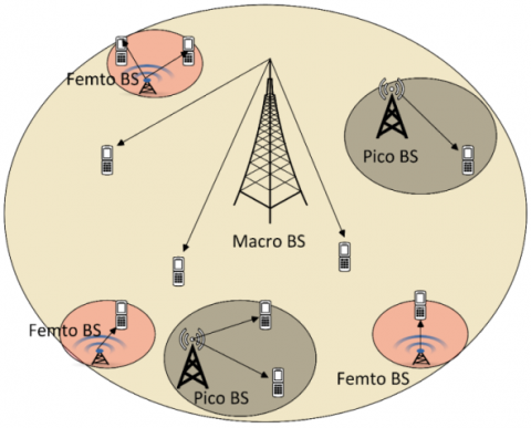
Standard multipath models applied at lower frequencies can be utilised to characterise the mmWave MIMO channel. Think of a MIMO system that uses Nr receive and Nt transmit antennas. The HetNets cell model has been shown in Figure 1.
aT(θT) and aR(θR) indicate array phase profile as a function of angular directions θR and θT of arriving or departing plane waves, respectively, and are used to define the transmit and receive antenna arrays in 2D channel models. The downlink channel model is displayed in Figure 2, which also shows the system architecture.
The steering vector for an N-element ULA is given by Eq. (9):
$a(\theta)=\left[1, e^{-j 2 \pi \vartheta}, e^{-j 4 \pi \vartheta}, \cdots, e^{-j 2 \pi v(N-1)}\right]^T$ (9)
In this case, normalised spatial angle ϑ is related to physical angle θ∈[−π/2, π/2] as ϑ=d λ sin(θ), where d stands for antenna spacing and for operating wavelength λ. Normally, d=λ/2 Steering vectors are functions a(θ, φ)=aaz(θ) ⊗ael(φ) of both horizontal angle θ and elevation angle φ in 3D channel methods. Given steering vectors, the multi-path model in Eq. (10) can be used to describe the MIMO channel.
$\mathbf{y}(t)=\sum_{\ell=1}^{N_0} \alpha_{\ell} e^{j 2 \pi v_{\ell} t} \mathbf{a}_{\mathrm{R}}\left(\theta_{\mathrm{R}, \ell}, \phi_{\mathrm{R}, \ell}\right) \mathbf{a}_{\mathrm{T}}^*\left(\theta_{\mathrm{T}, \ell}, \phi_{\mathrm{T}, \ell}\right) \mathbf{x}\left(t-\tau_{\ell}\right)+v(t)$ (10)
where, Np is the number of pathways, v(t) is noise vector, x(t) is transmitted signal vector, y(t) is received signal vector. Each path Lis defined by 5 parameters: The frequency domain representation of the channel is frequently helpful. The channel response is typically time-varying by Eq. (11):
$\begin{gathered}H(t, f)=\sum_{l=1}^{N_p} \alpha_l e^{j 2 \pi\left(v_l t-\tau_l f\right)} a_R\left(\theta_{R, l}, \phi_{R, l}\right) a_T^*\left(\theta_{T, l}, \phi_{T, l}\right) \cdot v_l T \ll 1 \\ H(f)=\sum_{l=1}^{N_p} \alpha_l e^{-j 2 \pi \tau_l f} a_R\left(\theta_{R, l}, \phi_{R, l}\right) a_T^*\left(\theta_{T, l}, \phi_{T, l}\right)\end{gathered}$ (11)
Assume that the channel varies sufficiently slowly throughout the signal period T, meaning that all of the pathways' Doppler shifts are tiny, $v_l T \ll 1 \forall l, l=1, \ldots, N_p$. (5) can then roughly be stated as Eq. (12):
Figure 1. HetNets cell model
Figure 2. The block diagram of a user and the BS
$\mathbf{H}(t, f)=\sum_{\ell=1}^{N_p} \alpha_{\ell} e^{j 2 t\left(v_r t-\tau_t f\right)} \mathrm{a}_{\mathrm{R}}\left(\theta_{\mathrm{R}, \ell}, \phi_{\mathrm{R}, \ell}\right) \operatorname{ar}^*\left(\theta_{\mathrm{T}, \ell}, \phi_{\mathrm{T}, \ell}\right)$ (12)
The narrowband spatial methods for channel matrix is obtained by Eq. (13) if the channel W's bandwidth is also sufficiently short such that τ`W 1∀`, `=1, ..., Np.
$\tau_l W \ll 1 \forall l, l=1, \ldots, N_p$ (13)
We have by Eq. (14) the received Tup block pilots stacked into a vector:
$y_{k, q} \triangleq\left[\frac{1}{x_{k, q, 1}} y_{k, q, 1}^T, \ldots, \frac{1}{x_{k, q, b}} y_{k, q, T}^T\right]^T=W_q^H h_{k, q}+W_q^H {n}_{k, q}^{\sim}$ (14)
$n_{k, q}^{\sim} \triangleq\left[\frac{1}{x_{k, q, 1}} n_{k, q, 1}^T, \ldots, \frac{1}{x_{k, q, \beta}} n_{k, q, T_{e p}}^T\right]^T \in C^{M T T_{q p} \times 1}$. Denote $h_k \triangleq\left[h_{k, p_{k, 1}}^T, \ldots, h_{k, p_{k, p}}^T\right]^T \in C^{M P \times 1}$. Collecting yk,q at different subcarriers, we have by Eq. (15):
$y_k \triangleq\left[y_{k, p_{k, 1}}^T, \ldots, y_{k, p_{k, p}}^T\right]^T=W^H h_k+n_k$ (15)
where,
$\mathbf{W} \triangleq\left[\begin{array}{cccc}\mathbf{W}_{p_{k, 1}} & 0 & \cdots & 0 \\ \mathbf{0} & \mathbf{W}_{p_{k, 2}} & \cdots & 0 \\ \vdots & \vdots & \ddots & \vdots \\ 0 & 0 & \cdots & \mathbf{W}_{p_{k, P}}\end{array}\right] \in \mathbb{C}^{M P \times N_{\mathrm{kF}} P T_{\bar{p}}}$ (16)
And the $\mathbf{n}_k \triangleq\left[\left(\hat{\mathbf{W}}_{p_{k, 1}}^H \tilde{\mathbf{n}}_{p k, 1}\right)^T, \ldots,\left(\hat{\mathbf{W}}_{p k, P}^H \tilde{\mathbf{n}}_{p k, p}\right)^T\right]^T \in \mathbb{C}^{N_{\mathrm{kr}} P T_{\mathrm{ep} \times 1}}$.
From (16), hk can be written as Eq. (17):
$h_k=\sum_{l=1}^{L_k} \alpha_{k, l} \mathbf{D}_k\left(\psi_{k, l}, \tau_{k, l}\right)_1$ (17)
where,
$p_k\left(\psi_{k, 1,}, T_{k, 1}\right) \triangleq\left[a^T\left(\Xi_{k, 1}\left(\left(p_{k, 1}-1\right) \eta\right)\right) e^{-j 2 \pi\left(p_{k, 1}-1\right) p n_{{k,1}_4}}\ldots, a^T\left(\Xi_{k, 1}\left(\left(p_{k, p}-1\right) \eta\right)\right) e^{-j 2 \pi\left(p_{k, p}, 1\right) \eta \eta, 1}\right]^T \in C^{M P \times 1}$ (18)
Eq. (18) is considered as channel basis for user k based on AoA $\psi_{k /}$ and path delay $\tau_{k, l}$. Denote $\alpha_k \triangleq\left[\alpha_{k, 1}, \ldots, \alpha_k, L_k\right]^T \in C^{L_k \times 1}$, $\psi_k \triangleq\left[\psi_{k, 1} \ldots, \psi_k, L_k\right]^T \in C^{L_k \times 1}$, and $\tau_k \triangleq\left[\tau_{k, 1}, \ldots, \tau_{k, l},\right]^T \in C^{L, k} \times 1$. Eq. (19) can be expressed in vector/matrix form as:
$h_k=P_k\left(\psi_k, \tau_k\right) \alpha_k$ (19)
where, by Eq. (20):
$P_k\left(\psi_k, \tau_k\right) \triangleq\left[p_k\left(\psi_{k, 1}, \tau_{k, 1}\right), \ldots, p_k\left(\psi_{k, L_k}, \tau_k, L_k\right)\right] \in C^{M P_{\times} L_k}$ (20)
Assume that the channel gains of the various multipath components are independent of one another and have a zero mean.
$E\left\{\alpha_k \alpha_k^H\right\}=\operatorname{diag}\left\{E\left\{\left|\alpha_{k, 1}\right|^2\right\} \ldots, E\left\{\left|\alpha_{k, L_k}\right|^2\right\}\right\} \triangleq \Lambda_k$ (21)
where, the average power of corresponding multipath component is $E\left\{\left|\alpha_{k, l}\right|^2\right\}$. Covariance matrix of uplink channel for user k is represented as Eq. (22) based on the description above.
$R_k^U \cong E\left\{h_k h_k^H\right\}=P_k\left(\psi_k, \tau_k\right) \Lambda_k P_k^H\left(\psi_k, \tau_k\right) \in C^{M P \times M P}$ (22)
As $rank\left(R_k^U\right) \leq {rank}\left(\Lambda_k\right)=L_k \& \Delta P$, $R_k^U$ is a pretty low-rank matrix. Given that $\frac{1}{\sqrt{M P}} P_k\left(\psi_k, T_k\right)$ is a tall matrix with unit-length asymptotically mutually orthogonal columns, Eq. (23):
$R_k^U=\left(\frac{1}{\sqrt{M P}} P_k\left(\psi_k, \tau_k\right)\right)\left(M P \Lambda_k\right)\left(\frac{1}{\sqrt{M P}} P_k^H\left(\psi_k, \tau_k\right)\right)$ (23)
Offers an accurate representation of eigenvalue decomposition. The received signals are projected to their respective signal subspaces at BS I where receive beamforming operations designed to eliminate intra-cell interference are subsequently carried out. After projection to signal subspace as well as reception beamforming, the received signal is given as Eq. (24):
$r_i=\left[r_{i, 1}, \cdots, r_{i, s}\right]^T=F_i^H U_i^H y_i$ (24)
In (25), the jth spatial stream, ri,j, is written as:
$r_{i, j}=\sqrt{P^{[i, j]}} x^{[i, j]} +\sum_{k=1, k \neq i}^K \sum_{m=1}^S \sqrt{P^{[k, m]}} \mathbf{f}_{i, j}^H \mathbf{U}_i^H \mathbf{H}_i^{[k, m]} \mathbf{W}^{[k, m]} \chi^{[k, m]} +\mathbf{f}_{i, j}^H \mathbf{U}_i^H \mathbf{z}_i .$ (25)
From (26), achievable rate of user j in BS i is given as:
$R^{[i, j]}=\log \left(1+\gamma^{[i, j]}\right)=\log \left(1+\frac{\mathrm{SNR}^{[i, j]}}{\left\|\mathbf{f}_{i, j}\right\|^2+I_{i, j}}\right)$ (26)
where, SINR γ[i,j] and the sum of residual interference of user j in BS i, are denoted. After ZF detection, the total residual interference can be expressed as Eq. (27):
$I_{i, j} \triangleq \sum_{k=1, k \neq i}^K \sum_{m=1}^S\left|\mathbf{f}_{i, j}^H \mathbf{U}_i^H \mathbf{H}_i^{[k, m]} \mathbf{w}^{[k, m]}\right|^2 \cdot \mathrm{SNR}^{[k, m]}$ (27)
From (28), total achievable DoF is described as follows:
$\mathrm{DoF}=\lim _{\mathrm{SNR} \rightarrow \infty} \frac{\sum_{i=1}^K \sum_{j=1}^S R^{[i, j]}}{\log _2 \frac{pmax }{N_0}}.$ (28)
3.2 Interference alignment using hybrid transfer convolutional network (HTCN)
Assume the HTC network, depicted in Figure 3, has N layers. The output is obtained in two phases for j-th node in layer I, designated as nij.zij j, the weighted total of all the inputs to node nij, is computed first. The output yij of node ni j via Eq. (29) is then obtained by sending zij to a non-linear function f ().
Figure 3. Architecture of HTCN
$z_{i j}=\sum_{i=1}^{L_i} w_{k j}^i y_{i j}=f\left(z_{i j}\right)$ (29)
where, Li-1 is number of nodes for layer i-1 and $w_{k j}^i$ is weight from node ni-1,k to node nij. Logistic function f(z)=1/[1+exp(-z)], hyperbolic tangent function f(z)={exp(z)-exp(-z)]/[exp(z)+exp(-z)], and ReLUf(z)=max(0, z), are all options for the non-linear function f(). are the preferred choices.
Backward error feedback: Initial weights are either empirical or random values. These weight values are modified using backward error feedback technique, which involves providing feedback on the classification accuracy to increase accuracy of learning methods final output. Error derivative is yNjtNj for a node of deepest layer, let's say node nNj, where yNj and tNj are generated output as well as correct output. Then lower layer connection error derivative by Eq. (30):
$\frac{\partial E}{\partial z_{N j}}=\frac{\partial E}{\partial y_{N j}} \frac{\partial y_{N j}}{\partial z_{N j}}$ (30)
where, $\partial E / \partial y_{N j}=y_{N j}-t_{N j}$ and j=1, 2, ⋯, LN. A weighted total of error derivatives of all inputs to j-th node of layer i(i=1, 2, ⋯, N-1), designated as ∂E/∂yij, is initially computed. Next, the lower layer connection's error derivative by Eq. (31):
$\frac{\partial E}{\partial z_{i j}}=\frac{\partial E}{\partial y_{i j}} \frac{\partial y_{i j}}{\partial z_{i j}}$ (31)
where, $\frac{\partial E}{\partial y_j j}=\sum_{k=1}^{L_{i+1}} w_{j k}^{i+1} \frac{\partial E}{\partial z=1, l}, i=1,2, \cdots, N-1$, and j=1, 2,⋯, Li.
The agent's objective is to maximise the total reward Qt via Eq. (32):
$\max _\pi Q_t=\max E_\pi\left(r_t+\gamma r_{t+1}+\gamma^2 r_{t+2}+\cdots \mid s_t=s, a_t=a, \pi\right)$ (32)
where, γ is a discount on future reward since present action at effects both the current reward and the future reward with decreasing strength. The agent randomly selects a sample of stored experience each time it needs to take an action throughout learning method. So, by Eq. (33):
$L_i\left(\theta_i\right)=E_{\left(s, a, r, s^{\prime}\right) \in U(D)}\left(\left(r+\gamma \max _{a^{\prime}} Q\left(s^{\prime}, a^{\prime}, \theta_i^{-}\right)-Q\left(s, a, \theta_i\right)\right)^2\right)$ (33)
NN is utilized to parameterize reward Q for each action, and each potential action is given its own output unit. Therefore, only state representation is used as input to network for each potential action, producing the projected Q value for a particular action.
Eq. (34) can be used to mathematically represent the optimization problem.
$\begin{gathered}\max _{P_{M D} \cdot P_{C D} \cdot P_{S U E}} g_o\left(P_{M D i}, P_{C D}, P_{S U E}\right) \text { s.t. } \gamma_{M B S} \geq T, 0 \\ \leq P_{M D i}, P_{C D}, P_{S U E} \leq P_{\text {max }}, i \\ \quad=1,2, \ldots, N\end{gathered}$ (34)
where,
$\begin{aligned} & g_o\left(P_{M D i}, P_{C D}, P_{S U E}\right)=\sum_{i=1}^N w_i \log _2\left(1+\gamma_{M D i}\right) +w_c \log _2\left(1+\gamma_{C D}\right) +w_s \log _2\left(1+\gamma_{S C B S}\right)\end{aligned}$ (35)
where, T is SINR threshold that gratifies MBS's minimum acceptable QoS and wi, wc, and ws are non-negative weights. The power PMUE is expressed in terms of powers of other users by Eqs. (36) and (37), utilizing lower bound to satisfy minimal QoS for MUE user.
$P_{\mathrm{MUE}}=\frac{\frac{h}{T}}{v-T v^{\prime}}\left(\sum_{i=1}^N q_i P_{\mathrm{MD} i}+r P_{\mathrm{CD}}+s P_{\mathrm{SUE}}+\sigma_{\mathrm{MBS}}^2\right)$
where,
$\begin{gathered}a_i^{\prime}=\alpha d_{\mathrm{MD} i}^\delta \\ b_i=d_{\mathrm{MD} i, \mathrm{CD}}^\delta\left[(1-\alpha)\left|\hat{h}_{\mathrm{MD} i, \mathrm{CD}}\right|^2+\alpha\right] \\ c_i=d_{\mathrm{MD} i, \mathrm{SUE}}^\delta\left[(1-\alpha)\left|\hat{h}_{\mathrm{MD} i, \mathrm{SUE}}\right|^2+\alpha\right] \\ d_i=d_{\mathrm{MD} i, \mathrm{MUE}}^\delta\left[(1-\alpha)\left|\hat{h}_{\mathrm{MD} i, \mathrm{MUE}}\right|^2+\alpha\right] \\ a_j^{\prime}=d_{\mathrm{MD} i, \mathrm{PMD} j}^\delta\left((1-\alpha)\left|\hat{h}_{\mathrm{MD} i, \mathrm{PMD} j}\right|^2+\alpha\right)\end{gathered}$
$\gamma_{\mathrm{CD}}=\frac{(1-\alpha)\left|\hat{h}_{\mathrm{CD}}\right|^2 d_{\mathrm{CD}}^\delta P_{\mathrm{CD}}}{e^{\prime} P_{\mathrm{CD}}+\sum_{i=1}^N f_i P_{\mathrm{MD} i}+g P_{\mathrm{SUE}}+h P_{\mathrm{MUE}}+\sigma_{\mathrm{CD}}^2}$ (36)
where,
$e^{\prime}=\alpha d_{\mathrm{CD}}^\delta, f_i=d_{\mathrm{CD}, \mathrm{MD} i}^\delta\left[(1-\alpha)\left|\hat{h}_{\mathrm{CD}, \mathrm{MD} i}\right|^2+\alpha\right], g=d_{\mathrm{CD} . \mathrm{SSUE}}^\delta\left[(1-\alpha)\left|\hat{h}_{\mathrm{CD}, \mathrm{SUE}}\right|^2+\alpha\right]$
$h=d_{\mathrm{CD} . \mathrm{MUE}}^\delta\left[(1-\alpha)\left|\hat{h}_{\mathrm{CD} . \mathrm{MUE}}\right|^2+\alpha\right]$
$\gamma_{\mathrm{SCBS}}=\frac{(1-\alpha)\left|\hat{h}_{\mathrm{SUE}}\right|^2 d_{\mathrm{SUE}}^\delta P_{\mathrm{SUE}}}{k^{\prime} P_{\mathrm{SUE}}+\sum_{i=1}^N l_i P_{\mathrm{MD} i}+m P_{\mathrm{CD}}+n P_{\mathrm{MUE}}+\sigma_{\mathrm{SCBS}}^2}$ (37)
where,
$k^{\prime}=\alpha d d_{\mathrm{SUE}}^\delta, l_i=d_{\mathrm{SCBS} . \mathrm{MDi}}^\delta[(1-\alpha) \mid \hat{h} \mathrm{SCBS}, \mathrm{MDi}+\alpha], m=d \delta_{\mathrm{SCBS.CD}}^\delta\left[(1-\alpha)\left|\hat{h}_{\mathrm{SCBS}, \mathrm{CD}}\right|^2+\alpha\right]$ and $n=d_{\text {SCBS.MUE: }}^\delta\left[(1-\alpha)\left|\hat{h}_{\text {SCBS.MUE }}\right|^2+\alpha\right]$.
$\gamma_{\mathrm{MBS}}=\frac{(1-\alpha)\left|\hat{h}_{\mathrm{MUE}}\right|^2 d_{\mathrm{MUE}}^{\delta_{\mathrm{M}}} P_{\mathrm{MUE}}}{v^{\prime} P_{\mathrm{MUE}}+\sum_{i=1}^N q_i P_{\mathrm{MD} i}+r P_{\mathrm{CD}}+s P_{\mathrm{SUE}}+\sigma_{\mathrm{MBS}}^2}$
where,
$v^{\prime}=\alpha d_{\mathrm{MUE},}^\delta q_i=d_{\mathrm{MBS}, \mathrm{MD} i}^{\check{\delta}}\left[(1-\alpha)\left|\hat{h}_{\mathrm{MBS}, \mathrm{MDi}}\right|^2+\alpha\right], r=d_{\mathrm{MBS}, \mathrm{CD}}^\delta\left[(1-\alpha)\left|\hat{h}_{\mathrm{MBS} . \mathrm{CD}}\right|^2+\alpha\right]$
$\gamma_{M D i}=\frac{(1-\alpha)\left|h_{M D i}^{\wedge}\right|^2 d_{M D_i}^\delta P_{M D i}}{\left(a_i^{\prime}+d_i h^{\prime} q_i\right)_{\underbrace{} \sigma_i^{\prime}} P_{M D i}+\left(\sum_{j=1 j \neq i}^N a_j^{\prime} P_{M D j}+d_i h^{\prime} \sum_{j=1 j \pm i}^N q_j P_{M D j}\right)}+\left(b_i+d_i h^{\prime} r\right)_{\underbrace{} b_i} P_{C D}+\left(c_i+d_i h^{\prime} s\right)_{\underbrace{} \epsilon_i^{\prime}} P_{S U E}+\sigma_{M D i}^2$
Next, the weighted sum of logarithms in issue is transformed using the Lagrangian dual transform.
$\max _{\boldsymbol{P}, \boldsymbol{\gamma}} g_{\delta_0}(\boldsymbol{P}, \boldsymbol{\gamma})$
s.t. $0 \leq P_{\mathrm{MD}}, P_{\mathrm{CD}}, P_{\mathrm{SUE}} \leq P_{\mathrm{max}}, k=(1-\alpha)\left|\hat{h}_{\mathrm{SUE}}\right|^2 d_{\mathrm{SUE}}^\delta \cdot \gamma_{\mathrm{MD}}, \gamma_{\mathrm{CD}}$, and γSCBS are introduced as an auxiliary variable introduced for every SINR ratio term, while P is set of $\left\{P_{M D}, P_{C D}, P_{S U E}\right\}$. The fractional SINR term is then moved outside of logarithm using quadratic transform, and all of the optimization variables are thus expressed in linear terms. The above reformulation is then used to create an iterative algorithm. The ideal value for P MD is equal to P MD when $P_{M D}, P_{C D}, \text{and } P_{S U E}$ are held constant. Setting $\partial g_0 / \partial \gamma_i, \partial g_0 / \partial \gamma_{C D}$, and $\frac{\partial g_0}{\partial \gamma_{S C B S}}$ to zero results in $\gamma=\gamma_{M D} \gamma_{C D}, \gamma_{S C B S}$. When powers PMD, PCD, and PSUE are kept constant, optimization of Pi only affects the terms of g 0 that have a sum-of-ratio form. When powers PMD, PCD, and PSUE are kept constant, the optimization of Pi only affects the terms of g0 that have a sum-of-ratio form. Because entire system performance depends on a number of fractional characteristics, the system in this situation must cope with various ratios.
This section assesses effectiveness of macro-small cellular network using PC methods with imprecise channel state data. Sum rate, coverage probability, and SINR are used to gauge performance. These simulations are performed using MATLAB software. The MBS is simulated as being at the centre of a single macro-cell. Within the cell radius, MUE and one MD pair are distributed at random. Considering uplink connection between cellular users as well as their matching BS, the SUE is considered to be situated near border of small-coverage cell's boundary. Additionally, a single CD pair is offered where its users are divided into various levels. It is expected that all simulation runs take place in an outdoor, typical metropolitan setting with stationary users. Table 1 lists the simulation parameters that were employed.
For uncoordinated interference with=0.8, we take into account faulty CSI. First, we begin with a case of (10 6, 4)3 MIMO interference with a single uncoordinated interference source with a transmit power of P1=0 dB. Additionally, for the proposed l2 and Schatten-p norm reduction techniques, we use Y=1d throughout this section. The average multiplexing gain (or DoF) is then depicted in Figure 2 is a function of the rank of uncoordinated interference, which runs from 1 to 4, when each user's transmit power is P=30 dB. The suggested strategies, as seen in the figure, boost average multiplexing gain, with the l2 norm minimization technique performing best in this case. It is also important to note that the suggested approaches perform significantly better than all other ways when the rank of uncoordinated interference is higher than 3. All other methods cannot deliver any average multiplexing advantage in this case. We take into account a (10 6, 4)3 MIMO interference system that has two uncoordinated interference sources. While keeping the rank of the second uncoordinated source fixed at 1, we depict the average multiplexing benefit as a function of the first uncoordinated source's rank. As can be shown, the proposed methods significantly outperform the other strategies. For instance, all existing strategies fail to achieve any average multiplexing advantage when the rank of the first uncoordinated source is equal to 2, but our suggested solutions significantly enhance IA performance. When our rank minimization method aims to reduce the interference's dimensional footprint, which raises the DoF, such gains are attained. The sum-rate also rises as a result, especially for medium and high SNR. On the other side, the Leakage Minimization technique seeks to reduce the interference's energy. However, compared to the rank minimization method, such lower-energy solutions result in a lower DoF. Additionally, the WMSE approach compromises the sum-rate by causing an unequal rate distribution among the users, with some transmitters having substantially lower rates than the others at medium and high SNR.
Table 1. Simulation specifications
|
Noise Spectral Density |
-174dBm/Hz |
|
Small Cell Radius |
20m |
|
Macrocell Radius |
500m |
|
System Bandwidth |
80MHz |
|
Estimation Error Variance a |
Varies between [0-1] |
|
Path Loss Coefficient |
4 |
|
D2D Range |
50m |
|
Initial Power Level Pinitial |
Pmax/2 |
|
Monto-Carlo Iterations |
10k |
|
Maximum Power Level Pmax |
23dBm |
Table 2. Comparative analysis between BER vs SNR
|
SNR |
LSFD |
DOA_MIMO |
HetNet_MUP_HTCN |
|
10 |
77 |
78 |
80 |
|
15 |
78 |
81 |
82 |
|
20 |
81 |
82 |
83 |
|
25 |
83 |
83 |
85 |
|
30 |
85 |
86 |
88 |
Figure 4. Comparative analysis for BER vs SNR
The above Table 2 and Figure 4 shows comparative analysis between BER vs SNR between proposed and existing technique. The amount of errors you are willing to accept is known as the bit error rate (BER). Usually, this is a value between 0.1 and 0.000001 (every 10th bit is terrible!) (Only one in a million is bad). This ratio and the decibel-measured SNR are closely related (dB). When BER decreases, the SNR rises, and vice versa when BER increases.
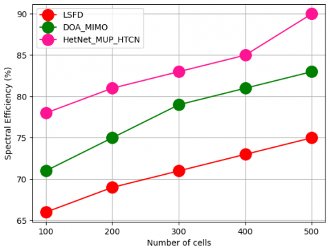
The below Table 3 and Figure 5 shows comparative analysis between proposed and existing technique in analyzing spectral efficiency. The maximum amount of data that are delivered to a specific number of users per sec while maintaining an acceptable QoS is the definition of spectral efficiency, also known as bandwidth efficiency or spectral capacity, in cellular networks.
Table 3. Comparative analysis of spectral efficiency
|
Number of Cells |
LSFD |
DOA_MIMO |
HetNet_MUP_HTCN |
|
100 |
66 |
71 |
78 |
|
200 |
69 |
75 |
81 |
|
300 |
71 |
79 |
83 |
|
400 |
73 |
81 |
85 |
|
500 |
75 |
83 |
90 |
A system's spectrum efficiency can be computed using the following formula if the channel bandwidth is 2 MHz and it can support a raw data rate of, say, 15 Mbps. If there is an overhead of 2 Mbps, net data rate is 13 Mbps. SE=13×106 / 2×106=6.5 bits/second/Hz.
Figure 5. Comparative analysis of spectral efficiency
Table 4. Comparative analysis of energy efficiency
|
Number of Cells |
LSFD |
DOA_MIMO |
HetNet_MUP_HTCN |
|
100 |
81 |
83 |
89 |
|
200 |
83 |
86 |
91 |
|
300 |
85 |
89 |
93 |
|
400 |
88 |
91 |
95 |
|
500 |
89 |
93 |
96 |
The Table 4 and Figure 6 show comparative analysis for energy efficiency between proposed and existing technique. The average rate per unit area to ratio of average power consumption per unit area can be used to calculate EE of a multicell uplink massive MIMO system. MIMO can support simple linear transceivers' high spectral efficiency (SE) and is anticipated to deliver excellent EE.
Figure 6. Comparative analysis of energy efficiency
Table 5. Comparative analysis of power consumption
|
Number of Cells |
LSFD |
DOA_MIMO |
HetNet_MUP_HTCN |
|
100 |
65 |
61 |
55 |
|
200 |
68 |
63 |
56 |
|
300 |
71 |
65 |
59 |
|
400 |
73 |
68 |
61 |
|
500 |
75 |
71 |
63 |
Table 5 and Figure 7 show comparative analysis of power consumption between proposed and existing technique. Power consumption model that takes into account base station residually lossy variables, analogue device circuit power dissipation, and transmit power on power amplifier (BSs). We evaluate tendency of EE as number of antennas increases as well as observe that EE through new EE formulation based on proposed power consumption method. For real power consumption method, RF circuit power consumption and transmission power consumption should be taken into account. Total power consumption likewise rises proportionally as number of transmit antennas grows because circuit power consumption does as well.
Figure 7. Comparative analysis of power consumption
It is simple to acquire the matrix that represents this linear mapping, and determining whether or not IA is feasible involves determining whether or not the matrix has full rank. Proper but impractical systems relate to situations where the input space's dimension and the solution variety's dimension coincide, but the mapping is not subjective, that is, the solution variety is mapped to a collection of zero-measure MIMO interference channels. We used a variety of instances to evaluate our feasibility test; some of them served to confirm previous findings, while others demonstrated the lack of tightness of the current DoF outer boundaries in this situation or offered proof of the benefits of using different-sized antennas and stream distribution to maximise the DoF. A thorough application of our test in symmetrical settings has enabled us to formulate a hypothesis on the DoF of the K-user interference channel that generalises previously established findings for K=3.
This research proposes novel technique in6G MIMO channel estimation with interference alignment based on heterogeneous network with deep learning techniques. here the channel estimation is carried out using HetNet based multiuser propagation model. the interference alignment of the network has been carried out using hybrid transfer convolutional network. However, as the effect of circuit power consumption is more severe when transmitter is outfitted with a large number of antennas. To determine precise power consumption of huge MIMO systems. Multiple cellular systems now support more energy-efficient communication as cellular method mounts large MIMO methods at BSs. We can determine ideal number of transmit antennas at BSs in relation to EE using results for the multi-cell system. The outcome of this research contributes to the well-organized installation of massive MIMO systems at BSs by emphasising importance of EE in communication networks. The proposed technique attained BER of 88%, spectral efficiency of 90%, energy efficiency of 96%, power consumption of 63%. In the future, we'll work to locate best active transmit antenna set, improve power consumption methods for EE, and resolve issue of user QoS restrictions such data rate requirements and communication dependability, among others. Future study may focus on discovering algorithms with reduced complexity that need less overhead, which is critical for big networks. Another intriguing future subject is creating completely distributed IA techniques, particularly for relay-aided settings.
[1] Kim, Y., Jung, B.C., Han, Y. (2022). Coordinated beamforming, interference-aware power control, and scheduling framework for 6G wireless networks. Journal of Communications and Networks, 24(3): 292-304. https://doi.org/10.23919/JCN.2022.000013
[2] Tekbıyık, K., Kurt, G.K., Huang, C., Ekti, A.R., Yanikomeroglu, H. (2021). Channel estimation for full-duplex RIS-assisted HAPS backhauling with graph attention networks. In ICC 2021-IEEE International Conference on Communications, pp. 1-6. https://doi.org/10.1109/ICC42927.2021.9500697
[3] Xu, Y., Gui, G., Gacanin, H., Adachi, F. (2021). A survey on resource allocation for 5G heterogeneous networks: Current research, future trends, and challenges. IEEE Communications Surveys & Tutorials, 23(2): 668-695. https://doi.org/10.1109/COMST.2021.3059896
[4] Najlah, C.P., Sameer, S.M. (2019). A GEVD based interference alignment method for uplink heterogeneous network under imperfect CSIT. In TENCON 2019-2019 IEEE Region 10 Conference (TENCON), pp. 835-840. https://doi.org/10.1109/TENCON.2019.8929704
[5] Sakr, H.M., Diab, A.M., Elamrawy, R., Elsabrouty, M.M. (2021). Experimental validation of interference alignment techniques for homogeneous and three-tier HetNets USING USRP-testbed. In 2021 38th National Radio Science Conference (NRSC), pp. 149-157. https://doi.org/10.1109/NRSC52299.2021.9509786
[6] Liu, W., Li, L., Jiao, L., Dai, H., Zheng, G. (2021). Joint interference alignment and probabilistic caching in MIMO small-cell networks. IEEE Transactions on Vehicular Technology, 70(9): 9400-9407. https://doi.org/10.1109/TVT.2021.3099157
[7] Prabakar, D., Sindhuja, R., Saminadan, V. (2019). Hybrid interference alignment (IA) scheme for improving the Sum-Rate of HetNet users. In 2019 2nd International Conference on Intelligent Computing, Instrumentation and Control Technologies (ICICICT), pp. 1095-1099. https://doi.org/10.1109/ICICICT46008.2019.8993187
[8] Wang, C., Deng, D., Xu, L., Wang, W., Gao, F. (2021). Joint interference alignment and power control for dense networks via deep reinforcement learning. IEEE Wireless Communications Letters, 10(5): 966-970. https://doi.org/10.1109/LWC.2021.3052079
[9] Pan, D., Li, B., Wang, C., Wang, W. (2019). Regional centralized interference alignment for multi-cell heterogeneous networks. In2019 IEEE 5th International Conference on Computer and Communications (ICCC), pp. 1430-1435. https://doi.org/10.1109/ICCC47050.2019.9064218
[10] Nasser, A., Muta, O., Elsabrouty, M., Gacanin, H. (2019). Interference mitigation and power allocation scheme for downlink MIMO–NOMA HetNet. IEEE Transactions on Vehicular Technology, 68(7): 6805-6816. https://doi.org/10.1109/TVT.2019.2918336
[11] Xu, Y., Li, J., Liu, W., Li, X., Liu, J., Peng, X. (2018). Cross-tier interference alignment with interfering pair selection in uplink heterogeneous networks with multiple macrocells. IEEE Access, 6: 28278-28289. https://doi.org/10.1109/ACCESS.2018.2836901
[12] Ren, Y., Zhang, X., Makhanbet, M. (2021). Interference alignment inspired opportunistic communications in multi-cluster MIMO networks with wireless power transfer. Information, 12(8): 335. https://doi.org/10.3390/info12080335
[13] Fanjul, J., Fernández, R.D., Ibáñez, J., García-Naya, J.A., Santamaria, I. (2020). Experimental evaluation of flexible duplexing in multi-tier MIMO networks. EURASIP Journal on Wireless Communications and Networking, 2020(1): 1-16. https://doi.org/10.1186/s13638-020-01799-x
[14] Mafuta, A.D., Walingo, T. (2018). Interference alignment for transceiver design in multi-user MIMO relay system. In2018 IEEE 88th Vehicular Technology Conference (VTC-Fall), pp. 1-5. https://doi.org/10.1109/VTCFall.2018.8690601
[15] Ranjith, S., Jayarin, P.J., Sekar, A.C. (2023). A multi-fusion integrated end-to-end deep kernel CNN based channel estimation for hybrid range UM-MIMO 6G communication systems. Applied Acoustics, 210: 109427. https://doi.org/10.1016/j.apacoust.2023.109427
[16] Benaya, A.M., Elsabrouty, M. (2019). Opportunistic interference alignment for three‐tier partially connected heterogeneous networks. International Journal of Communication Systems, 32(12): e4009. https://doi.org/10.1002/dac.4009
[17] Wang, B., Jian, M., Gao, F., Li, G.Y., Lin, H. (2019). Beam squint and channel estimation for wideband mmWave massive MIMO-OFDM systems. IEEE Transactions on Signal Processing, 67(23): 5893-5908. https://doi.org/10.1109/TSP.2019.2949502
[18] Qamar, F., Hindia, M.H.D., Dimyati, K., Noordin, K.A., Amiri, I.S. (2019). Interference management issues for the future 5G network: A review. Telecommunication Systems, 71(4): 627-643. https://doi.org/10.1007/s11235-019-00578-4
[19] Suo, L., Li, H., Zhang, S., Li, J. (2022). Successive interference cancellation and alignment in K-user MIMO interference channels with partial unidirectional strong interference. China Communications, 19(2): 118-130. https://doi.org/10.23919/JCC.2022.02.010
[20] Muta, O., Hao, W., Gacanin, H. (2018). Pilot allocation and interference coordination for heterogeneous network with massive MIMO/TDD. In 2018 International Symposium on Intelligent Signal Processing and Communication Systems (ISPACS), pp. 295-300. https://doi.org/10.1109/ISPACS.2018.8923182
[21] Liu, W., Zhang, Z., Huang, L., Xu, J., Chen, X. (2021). Alignment chain-based closed-form IA solution for multiple user MIMO interference networks. IEEE Transactions on Vehicular Technology, 70(2): 1518-1527. https://doi.org/10.1109/TVT.2021.3053606
[22] Ali, S.S., Castanheira, D., Alsohaily, A., Sousa, E., Silva, A., Gameiro, A. (2018). Two-tier cellular system up-link based on space-frequency block codes and signal alignment. In 2018 IEEE Wireless Communications and Networking Conference (WCNC), pp. 1-5. https://doi.org/10.1109/WCNC.2018.8377026
[23] Najlah, C.P., Sameer, S.M. (2021). A NOMA scheme using oblique projection for hetnet uplink under perfect and imperfect CSIR. IEEE Transactions on Vehicular Technology, 70(3): 2673-2683. https://doi.org/10.1109/TVT.2021.3062065
[24] Rajoria, S., Trivedi, A., Godfrey, W.W. (2021). Sum-rate optimization for NOMA based two-tier hetnets with massive MIMO enabled wireless backhauling. AEU-International Journal of Electronics and Communications, 132: 153626. https://doi.org/10.1016/j.aeue.2021.153626
[25] Mellempudi, G.K., Pamula, V.K. (2019). Channel estimation using adaptive cuckoo search based wiener filter. In International Symposium on Signal Processing and Intelligent Recognition Systems, pp. 332-346. https://doi.org/ 10.1007/978-981-15-4828-4_27