Huali Jiang*![]() | Xin Li
| Xin Li![]()
© 2023 IIETA. This article is published by IIETA and is licensed under the CC BY 4.0 license (http://creativecommons.org/licenses/by/4.0/).
OPEN ACCESS
Moving object detection from video sequences remains a focal point of research. To address the limitations evident in current methodologies, a synthesis of optical flow method and salient object fusion algorithm has been applied. Utilising the Graph-based Visual Saliency (GBVS) algorithm, significant target region signals from both static and dynamic images can be obtained. This technique captures valuable image target information, highlighting conspicuous targets within dynamic visuals. Concurrently, target signals can be isolated employing the Harmony Search (HS) algorithm, enhancing the accuracy in identifying moving objects. A weighted fusion of the extracted salient regions by the GBVS algorithm and the moving objects identified by the HS algorithm was executed in this study. This amalgamation demonstrates efficacy in extracting static objects in rudimentary environments and complex backgrounds alike. MATLAB simulation experiments have indicated that such a multi-modal fusion not only diminishes background noise but also proficiently isolates the entirety of the target. Building on traditional frame difference and background difference methods and considering the properties of the field programmable gate array (FPGA) alongside off-chip synchronous dynamic memory's access control prerequisites, adaptations for these algorithms were conceived using FPGA logic units.
Harmony Search algorithm, Graph-based Visual Saliency algorithm, multi-modal fusion, MATLAB
In today's digital age, a staggering volume of information is encountered daily. It has been documented that over 75% of all perceived information is acquired through human vision [1]. Video target detection, a paramount research direction within the realm of computer vision, has traditionally focused on the minutiae of images or enhancing their visibility. However, during the image acquisition phase, numerous interference factors such as variable weather conditions, lighting discrepancies, environmental noise, and extraneous disturbances like insect interference have been identified [2]. Challenges such as indistinct targets, excessive motion speeds, overlapping of targets, and irregular object shapes have been encountered. Addressing these issues and refining the detection in complex backgrounds has been deemed essential.
The prevailing approach in target detection has been the utilisation of moving target detection anchored in machine learning. Pedestrian features, encompassing texture, colour, and various gradient metrics like Histogram of Oriented Gradients (HOG) [3], Haar features, Scale Invariant Features (SIFT), and Speeded Up Robust Features (SURF) have been meticulously designed. Efficient feature classifiers, including Support Vector Machine (SVM) [4], random forests, and deep learning methodologies, have been employed to achieve precision in pedestrian detection. The predominant method involves extracting the HOG of distinct blocks within a sample or detection window, followed by training to attain an SVM [5] classifier. The codebook background modelling algorithm has been introduced, which facilitates the extraction of pedestrian foreground images. This substantially minimises the search ambit during retrieval, and the application of random forest methodologies, coupled with Haar and HOG features, have been observed for training and classification.
With the swift progression of microelectronics technology in recent years, a surge in demand for advanced machine vision has been noted. Despite significant advancements, considerable potential for enhancement remains, particularly in resolution and processing speed. Moving object detection technology, with its extensive applications in sectors like artificial intelligence, healthcare, and security, has grown pivotal. A pressing need for a framework capable of real-time processing of moving images has emerged. While contemporary CPU frequencies approach the GHz range, certain scenarios with intensive computational demands, such as real-time tracking of mobile targets or concurrent multi-target tracking, transcend the capabilities of standard computing systems.
In the process of video sequence information extraction, the foremost step is typically the extraction of requisite target information for detection. From daily observations, it has been discerned that target detection permeates various sectors. Within the expansive field of vision detection, target detection stands out as a cornerstone. Targets, based on background dynamics, have been broadly categorised into two: those with static backgrounds and those embedded in moving backgrounds [6]. The latter, characterised by significant fluctuations and numerous interfering elements, poses an amplified challenge due to simultaneous target and background alterations.
Historically, in the 1970s, inter-frame difference methods [7, 8] were introduced, and a mathematical model for video sequence background information was formulated, using a singular Gaussian model. Stauffer et al. [8-10] subsequently expanded on this by proposing the Gaussian mixture model, a method now widely recognised. Efforts were also made by Gorelick et al. [10, 11] in motion compensation post background region segmentation and the exploration of optical flow methods. Over extended periods, the human visual system evolved to adeptly locate objects of interest in both static and dynamic environments, a capability attributed to a rapid visual selection mechanism [12].
It has been observed that moving objects induce grayscale variations in images. These alterations manifest as optical flow changes, with the moving saliency map delineating the prominence of such flows. In the context of observing images, the visual system is naturally drawn to salient regions, indicative of visual saliency [13]. Amidst complex environments, the visual attention mechanism serves to allocate limited neural resources to areas of interest [14-17]. Notably, in the 1980s, a plethora of foundational theories on visual attention were postulated. Treisman and Gelade [18] proposed the feature integration theory, underscoring the importance of attention to visual features. Koch and Ullman [19] expanded upon this, introducing a bottom-up research mechanism and advocating for an augmented description of scene saliency through visual feature graph amalgamation. Further, Itti et al. [20] actualised the bio-inspired model earlier suggested by Koch and Ullman [19]. It has been noted that the human visual attention mechanism operates in two primary phases: bottom-up and top-down processes [18, 19].
Applications of visual saliency detection technology have been diverse. First, image and video compression [20]. Compression [20] processes traditionally demand intensive computations. During such operations, both near lossless and lossless compression predominantly target non-significant regions, consequently economising computational resources. Meanwhile, lossy compression balances quality preservation with an enhanced compression ratio. Second, image search process [21]. The essence of this application lies in content comparison. By juxtaposing salient areas within image contents and contrasting visual attributes, the congruence of salient regions becomes instrumental in gauging content similarity. Third, image segmentation [22]. The inherent robustness of visual saliency against noise has been employed to tackle challenges in differentiating targets from backgrounds in traditional imaging. Finally, automatic target detection [23]. This process essentially constitutes the sequential identification of visually significant areas, ensuring that the recognition efficiency remains unimpaired by non-salient regions.
In-depth examinations have illuminated the profound congruence between visual saliency detection technology and human vision principles. Such systems are believed to optimise image processing efficiency, holding both theoretical and practical significance for advancing the scientific domain. Yet, from contemporary outcomes of visual saliency detection methodologies, it is evident that issues of accuracy and precision remain to be refined to ensure the efficacy of visual system processing.
Although dynamic background detection predominantly incorporates block matching methods [24] and optical flow estimation methods [25], this section emphasizes a comparative simulation of three quintessential techniques relevant to static backgrounds.
3.1 Frame difference method
Figure 1. Illustration of the difference method
In the inter-frame difference approach, two consecutive frames from a video sequence are initially read. The edge contours of moving objects within these frames are then distinguished. Given the consistent shooting interval, the background is presumed static. A disparity between two successive frames indicates motion, and any alterations between them suggest the presence of moving objects. An established threshold aids in automatically recognising these moving objects by contrasting the two frames. For this simulation, frames 149 and 150 from an avi video format were employed, both in their original colour and after grayscale processing. As exhibited in the figure, frames 149 and 150 represent the initial colour frames (Figure 1). Considering minimal changes typically exist between sequential video frames, the presence of moving objects across two consecutive frames results in content alterations. By distinguishing the edge contours of moving objects between these frames, an inter-frame difference binary image is derived. Subsequent morphological operations further enhance the clarity of the results.
3.2 Background difference method
Figure 2. Illustration of the background difference method
The figure-background difference method serves as an alternative approach for detecting moving objects (Figure 2). In this technique, a parameter model of the background image difference within a moving video sequence is employed. Typically, the pixel difference of the background image is characterised using a predefined parameter model. Subsequently, a calculation is made to compare the difference between the current image and the mathematical model of the established background. Moving objects are delineated based on the degree of change observed. Regions with significant differences are classified as areas containing moving objects. In contrast, zones with negligible differences are categorised as the background. It is crucial to underscore that an image devoid of any moving objects forms the background. Moreover, there's a continual need to adapt the background model to accommodate background transformations [26]. The light flow method, while not directly connected to the scene, primarily hinges on the disparity between the velocity vectors of the background and the target. This method facilitates the determination of the velocity of an independent moving target [27].
Figure 3. Background difference simulation diagram
Figure 3 showcases a MATLAB simulation of the inter-frame difference method. The 150th frame of colour images in the avi format was utilised. The depiction includes: (a) the original 150th frame of the video in colour, (b) the background image post grayscale conversion, (c) a representation where the pixel difference of background images is delineated by the established parameter model. In this representation, foreground computations are undertaken, foreground pixels are retained, and the background is updated. Regions with pronounced differences signify the range of the moving target, whereas areas with minimal differences represent the moving background. The culmination of these steps results in the final image.
3.3 Optical flow method
When both a camera and its target are in motion simultaneously, an evolving image is generated on the camera's final imaging plane. Due to irregularities in the object's surface lighting, the relative movement between the camera and the object induces variations in illumination. These fluctuations in illumination are referred to as light flow [28]. The optical flow method, pivotal in video analysis, is designed to detect the instantaneous velocity of moving target pixels. The aim of this method is to estimate the actual three-dimensional motion through the two-dimensional velocity field [29]. Utilising the optical flow method to acquire information on moving targets can mitigate challenges introduced by irregular object movements or background noise. Nonetheless, under conditions of significant auditory noise or abrupt lighting changes, the detection results derived from the optical flow method can occasionally manifest substantial inaccuracies. Rapidly altering backgrounds can be problematic for differentiation solely based on image variations. However, when backgrounds remain static or change slowly, the results are notably discernible. The optical flow field's pixel density can be divided into three categories. First, dense optical flow method. In this approach, each point within a designated area is individually analysed for light loss, requiring point-by-point matching. This method demands a considerable computational load, complicating target tracking. Second, sparse optical flow method. Only points with distinguishable features that satisfy specific conditions are selected for analysis, eliminating the need for point-by-point matching. Finally, semi-dense optical flow. Building upon the sparse method, this technique introduces unique points. The light loss of these points is then calculated to enhance gradient visibility.
Optical flow method can be broadly subdivided into five types based on their calculation methods: First, gradient method. Image brightness remains constant, converting the image to grayscale, subsequently facilitating the calculation of pixel velocity vectors. Second, region matching method [30]. Either through region or feature matching, this approach processes video sequences to locate, track, and derive useful displacements of moving targets. All identified valid displacements represent target motion vectors. Third, frequency calculation method. Employing an adjustable speed filter, images are processed using a spatio-temporal filter. This approach amalgamates time and space processes to estimate velocity vectors in a consistent flow field accurately, yielding both frequency and phase data. Fourth, phase calculation method. Determining the optical flow field through image phase phase-related calculations. Even during environmental emergencies or disruptions, this method maintains performance, making it preferable when selecting brightness data in exceptional scenarios. Finally, neurodynamic calculation method [31]. The neurodynamic model of visual motion perception, constructed using neural networks, emulates the function and structure of biological visual systems.
The differential method, a technique derived from global energy functionals, utilises the spatial gradient function over a unit time to ascertain the minimum value, subsequently calculating the image time vector. Characterised by its rigorous logical design, the differential method finds support in numerous conceptual frameworks. Given that gradient-based algorithms hold the distinction of being amongst the most classical computational techniques, the term "differential method" often serves as a direct abbreviation. In everyday discourse, this abbreviation is frequently adopted. Among the myriad of methods available for optical flow computation, the differential method is reported to be the most extensively studied and commonly employed in standard experiments [32].
In 1950, Gibson [33] introduced the concept of an instantaneous velocity of image flow on a target's imaging surface, defining the surface velocity of image flow in grayscale mode [34]. Later, in 1981, the optical flow method was postulated by American scientists Horn and Sehunck [35, 36]. They emphasized optical flow as a representation of object motion, deriving the foundational optical flow constraint equation based on image conservation theory. The implementation of the optical flow method is contingent upon three primary assumptions. First, brightness across adjacent frames remains invariant. Second, adjacent frames exhibit notable target motion amplitude. Finally, spatial consistency is maintained across adjacent frames. The HS algorithm, also termed the dense optical flow method, incorporates an overarching assumption of zero velocity change, producing a relatively smooth optical flow field.
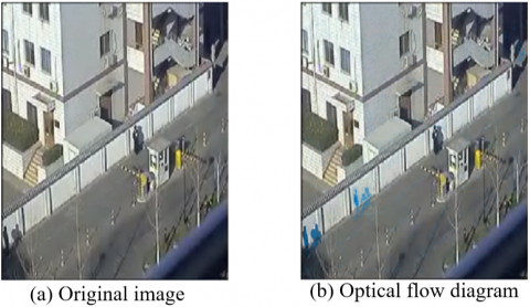
In Figure 4, a simulation diagram of the MATLAB optical flow method is presented. This .avi video format sequentially displays two images, with an intentional selection of two frames showcasing significant differences to underscore the methodology's effectiveness (Figure 5).
Figure 4. Optical flow methodology
Figure 5. Optical flow vector diagram
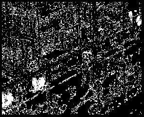
Figure 6. Results of optical flow binarization
Figure 6 portrays the resultant binarization of the optical flow for the image, highlighting moving objects through enhanced white areas. Despite prevalent interference elements within the image, discernible movement of objects against a static backdrop is evident.
Consider a pixel, denoted as I(x,y,t), positioned at (x, y) in an image at time T. Should this pixel undergo a movement by ΔxΔy after a duration Δt, its behaviour can be expressed using the Taylor series expansion, as follows:
$I\left( x+\Delta x,y+\Delta y,t+\Delta t \right)=I\left( x,y,t \right)+\frac{\partial I}{\partial x}\Delta x+\frac{\partial I}{\partial y}\Delta y+\frac{\partial I}{\partial t}\Delta t+\sigma $ (1)
Under the assumption that the grey level remains constant over time, the equation can be represented as:
$I\left( x+\Delta x,y+\Delta y,t+\Delta t \right)=I\left( x,y,t \right)$ (2)
σ is the second-order and higher-order terms representing Δt, Δy and Δx can be obtained from the above formula:
$\frac{\Delta x}{\Delta t}\frac{\Delta I}{\Delta x}+\frac{\Delta y}{\Delta t}\frac{\Delta I}{\Delta y}+\frac{\Delta I}{\Delta t}+o\left( \Delta t \right)=0$ (3)
Analysing the derived formulae, it is observed that both Δx and Δy display variations in relation to Δt. Consequently, as Δt approaches zero, the ensuing behaviour is deduced:
$\frac{\partial I}{\partial x}\frac{dx}{dt}+\frac{\partial I}{\partial y}\frac{dy}{dt}+\frac{\partial I}{\partial t}=0$ (4)
u, v is the velocity component in both horizontal and vertical directions. From this representation, the following has been derived:
$I_xu+I_yu+It=0$ (5)
This equation is recognised as the fundamental optical flow constraint equation. It elucidates the intrinsic relationship between time, spatial attributes, and velocity inherent in moving entities. Through this understanding, the intensity diminution across the entire range of images has been determined.
A novel smoothing constraint was introduced by Horn et al. with the aim of enhancing the homogeneity of optical flow. This constraint sought to minimise the parameter Es. The specified smoothing constraints are given as:
${{E}_{\text{s}}}={{\left[ {{\left( \frac{\partial u}{\partial x} \right)}^{2}}+{{\left( \frac{\partial u}{\partial y} \right)}^{2}}+{{\left( \frac{\partial v}{\partial x} \right)}^{2}}+{{\left( \frac{\partial v}{\partial y} \right)}^{2}} \right]}^{2}}dxdy$ (6)
Employing the fundamental optical flow equation, an avenue for minimising the optical flow error has been identified:
${{E}_{c}}={{\left( {{I}_{x}}u+{{I}_{y}}v+{{I}_{t}} \right)}^{2}}dxdy$ (7)
When the constraints highlighted in the two preceding equations are evaluated, it is discerned that the calculated light loss should adhere to particular stipulations.
${{E}_{s}}=\left\{ {{\left( {{I}_{x}}u+{{I}_{y}}v+{{I}_{t}} \right)}^{2}}+\lambda {{\left[ \begin{align} & {{\left( \frac{\partial u}{\partial x} \right)}^{2}}+{{\left( \frac{\partial u}{\partial y} \right)}^{2}} \\ & +{{\left( \frac{\partial v}{\partial x} \right)}^{2}}+{{\left( \frac{\partial v}{\partial y} \right)}^{2}} \\\end{align} \right]}^{2}} \right\}dxdy=min$ (8)
When confronted with pronounced image noise, confidence levels tend to diminish. Under such circumstances, it has been observed that the adoption of a more substantial weight coefficient is judicious. Superior image quality invariably leads to enhanced precision in computations. A diminutive weight coefficient, on the other hand, can potentially curtail the reliance on smoothing conditions. Pertaining to derivatives, the following equations are presented:
${{I}^{2}}_{x}u+{{I}_{x}}{{I}_{y}}v=-{{\lambda }^{2}}\nabla u-{{I}_{x}}{{I}_{t}}$ (9)
${{I}^{2}}_{y}v+{{I}_{x}}{{I}_{y}}u=-{{\lambda }^{2}}\nabla v-{{I}_{y}}{{I}_{t}}$ (10)
Values $\bar{u}$ and $\bar{v}$ are discerned as the mean values, while further relations with $\nabla u=u-\bar{u}$ and $\nabla v=v-\bar{v}$ are explicated in:
$\left( {{\lambda }^{2}}+{{I}^{2}}_{x} \right)u+{{I}_{x}}{{I}_{y}}v=-{{\lambda }^{2}}\bar{u}-{{I}_{x}}{{I}_{t}}$ (11)
$\left( {{\lambda }^{2}}+{{I}^{2}}_{y} \right)v+{{I}_{x}}{{I}_{y}}u=-{{\lambda }^{2}}\bar{v}-{{I}_{x}}{{I}_{y}}$ (12)
By coalescing Eqs. (5) and (7), the subsequent results are procured:
$u=\bar{u}-\frac{{{I}_{x}}\bar{u}+{{I}_{y}}\bar{v}+{{I}_{t}}}{{{\lambda }^{2}}+{{I}^{2}}_{x}+{{I}^{2}}_{y}}$ (13)
$v=\bar{v}-\frac{{{I}_{x}}\bar{u}+{{I}_{y}}\bar{v}+{{I}_{t}}}{{{\lambda }^{2}}+{{I}^{2}}_{x}+{{I}^{2}}_{y}}$ (14)
The relaxation iteration method furnishes solutions as:
${{u}^{\left( n+1 \right)}}={{\bar{u}}^{\left( n \right)}}-\frac{{{I}_{x}}{{{\bar{u}}}^{\left( n \right)}}+{{I}_{y}}{{{\bar{v}}}^{_{\left( n \right)}}}+{{I}_{t}}}{{{\lambda }^{2}}+{{I}^{2}}_{x}+{{I}^{2}}_{y}}$ (15)
${{v}^{\left( n+1 \right)}}={{\bar{v}}^{\left( n \right)}}-\frac{{{I}_{x}}{{{\bar{u}}}^{\left( n \right)}}+{{I}_{y}}{{{\bar{v}}}^{_{\left( n \right)}}}+{{I}_{t}}}{{{\lambda }^{2}}+{{I}^{2}}_{x}+{{I}^{2}}_{y}}$ (16)
This method is widely acknowledged as the HS optical flow method. Standard practice dictates the initial light loss value to be configured as (0,0). For achieving commendable accuracy, it has been noted that iterations often surpass the count of 20.
In environments with intricate visual backgrounds and multiple target objects, the primary intrigue often gravitates towards objects of interest. These objects are swiftly and precisely identified amongst prominent target entities. Such behavioural patterns are referred to as the visual attention mechanism. The human visual system, refined over extended evolutionary periods, doesn't merely process information straightforwardly; rather, it undergoes multiple intricate phases. The intricacy of this system not only pertains to its detailed nature but also its complexity. A myriad of stages is often navigated to actualise a comprehensive visual system. The inherent finesse of this mechanism is manifested in the judicious allocation of resources. During computational processing of videos, non-essential information is habitually disregarded, thereby reducing computational demands. The focus is intensified on pertinent information, thus endorsing the efficacy of employing human visual system mechanisms in realms such as target recognition, image compression, and retrieval.
The attention mechanism encompasses three pivotal components: bottom-up, top-down, and the attention inhibition principle. The bottom-up mechanism is a data-driven detection mode that operates devoid of pre-existing experiential knowledge. Through the synthesis of psychological theory and cognitive neuroscience, a hypothetical system is constructed, and a computation library is designed to emulate the human visual system's functionality. In contrast, the top-down mechanism necessitates pre-existing empirical knowledge of semantic feature location. Before employing this approach, it is imperative that target features and specific tasks are pre-defined.
4.1 Calculation principles
The simulation of visual salience mirrors the biological visual attention mechanism, necessitating adherence to its inherent principles. Several axioms underlie visual attention, including several principles. First, centre-neighbourhood principle [34]. It is observed that the visual centre is the most sensitive region for visual neurons. External stimuli typically either augment or diminish this sensitivity, accentuating the contrast between centres and their surroundings. Second, principle of high-frequency occurrence inhibition. This principle asserts that the visual system tends to overlook recurring features, directing its focus towards anomalous attributes. This proclivity explains the human tendency to be captivated by conspicuous objects. Saliency detection models, especially those based on statistical paradigms, often harness these anomalous features for modelling. Third, two-colour opposition principle. Drawing from the differential responses of the cerebral cortex to identical wavelength light stimulations, this principle underlines the cerebral cortex's contrasting reactions to varying wavelengths. It stands as a foundational pillar of early colour saliency theories. Finally, principle of contrast. Objects are frequently contrasted against their respective backdrops. Two distinct variants of this principle exist. Global contrast necessitates the computation of disparities between every pixel and the overall scene, entailing substantial computational demands. Conversely, local contrast exclusively quantifies the deviation between a centre and its immediate periphery, thereby minimising computational requirements.
Regarding saliency analysis algorithms, three prevalent methodologies are identified. Firstly, algorithms grounded in the low-level visual information system, with the Itti algorithm serving as a quintessential exemplar. The second category encompasses methods such as the AC and SR algorithms. The third paradigm synthesises elements from the former methodologies, epitomised by the graph theory-based GBVS algorithm. This algorithm exclusively employs mathematical computations to discern saliency values.
4.2 Analysis of the GBVS algorithm
Given an object $M:[n]^2 \rightarrow R$, feature extraction is performed either through localisation of $A:[n]^2 \rightarrow R$, or by employing a node M(i,j). In the Bruce algorithm, the histogram automatically computes the proportion of diverse features in the vicinity of nodes containing unprocessed information. This procedure is continued until a probability distribution map is derived from the feature map.
Given the formulas:
$A\left( i,j \right)=-\log \left( p\left( i,j \right) \right)$ (17)
$p\left( i,j \right)=\Pr \left\{ M\left( i,j \right)\left| neighborhood \right. \right\}$ (18)
The disparity between M(i,j) and M(p,q) is determined through the subsequent equations:
$d\left( \left( i,j \right)\left\| \left( p,q \right) \right. \right)\underline{\underline{\Delta }}\left| \log \frac{M\left( i,j \right)}{M\left( p,q \right)} \right|$ (19)
${{w}_{1}}\left( \left( i,j \right),\left( p,q \right) \right)\underline{\underline{\Delta }}d\left( \left( i,j \right)\left\| \left( p,q \right) \right. \right)\cdot F\left( i-p,j-q \right)$ (20)
$F\left( a,b \right)\underline{\underline{\Delta }}exp\left( -\frac{{{a}^{2}}+{{b}^{2}}}{2{{\sigma }^{2}}} \right)$ (21)
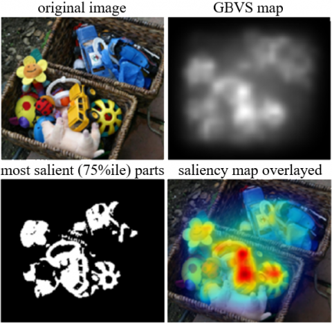
Figure 7. Illustration of saliency in complex background
In these equations, σ represents a free variable. Following numerous iterations, a stable distribution is attained. The lesser the visual feature similarity between nodes, the larger the weight. This leads to an increased probability of state transition, culminating in an extended accumulation period on the respective node. Conversely, when similarities are pronounced, the accumulation period is abbreviated. A marked difference in visual characteristics highlights their significance. The principal eigenvector of the Markov matrix corresponds to the eigenvalues of the primary level. Moreover, the eigenvalues of the level variables exhibiting the maximum modulus among the matrix's eigenvalues are also denoted as primary eigenvalues. These correspond to the most pivotal nodes on the graph. Subsequent to this, the relation system of the principal eigenvector materialises as a two-dimensional graph.
Figure 7 portrays the saliency map's simulation against intricate backgrounds. The initial diagram presents the native colour image, succeeded by a grayscale rendition processed via the GBVS algorithm. The subsequent illustration provides a binary representation of the GBVS-processed grayscale image. The final representation superimposes the saliency region onto the original image, thus offering a more lucid visualisation of the salient region.
Figure 8. Saliency display in simple background
In contrast, Figure 8 delineates the saliency map's simulation against more rudimentary backgrounds. The sequence of illustrations mirrors that of Figure 8, culminating in an overlay of the saliency region on the original image for enhanced visual clarity.
When juxtaposed, the saliency maps of Figure 8 (complex background) with Figure 9 (simple background) evince that the GBVS algorithm's simulation is predisposed to produce nebulous and imprecise saliency maps in intricate environments. In stark contrast, salient figures extracted from visuals characterised by unadorned backgrounds and conspicuous targets are relatively more coherent. In general terms, the detection outcomes from the GBVS algorithm are susceptible to misinterpretation, erroneously identifying irrelevant positions within the backdrop as salient regions. This often culminates in an expansive nebulous zone, compromising the overall detection efficacy. Conversely, the detection precision in simpler background proves superior.
4.3 Weighted fusion algorithm
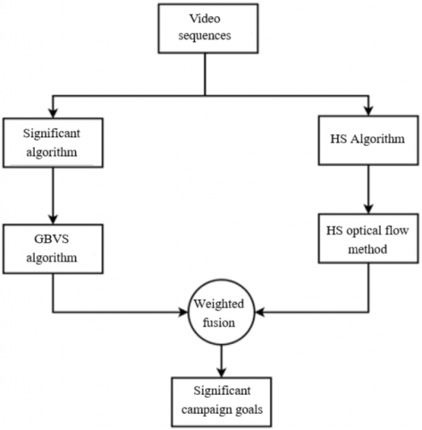
The algorithm's primary notion surrounding the detection of salient moving objects can be distilled as follows: Initially, a video sequence is acquired. Subsequently, saliency detection is undertaken using the GBVS algorithm, culminating in the segregation and reconstruction of salient moving objects. Concurrently, the HS optical flow algorithm is employed to dissect two consecutive frames of the video sequence, thus enabling the identification of the salient moving objects. In the final step, the discerned salient information is amalgamated with the motion data, resulting in the extraction of salient moving objects.
Figure 9. Flow chart depicting convergence
As depicted in the aforementioned figure, the GBVS algorithm's application to the first video frame yields the salient object. The optical flow method, when applied to the initial two frames of the video sequence, discerns the moving object. The culmination of this process sees the fusion of the moving object with the salient object.
The optical flow vector of the ongoing video frame, in both X and Y directions, can be computed through Eqs. (15) and (16). The optical flow field at the specific point is then ascertained through the root mean square, as denoted in Eq. (22):
$V=\sqrt{{{v}_{x}}^{2}+{{v}_{y}}^{2}}$ (22)
The resultant regional saliency computations are integrated with the target optical flow field from Eq. (22), as depicted in Eq. (23). Within this equation, the weight value is adjustable contingent on experimental outcomes, typically oscillating between 0.8 and 1.5. β is the weight value. That is, S is the salient image obtained by using GBVS algorithm in MATLAB.
$G=\beta \cdot \left( V*S \right)+S$ (23)
In the context of Eq. (23), it is observed that the saliency map attenuates the background domain within the optical flow vector. Subsequent weighted fusion of the two values augments the range while diminishing the background interference, thereby achieving the desired detection target.
Comparative results using different β values have illuminated the influence on image luminance, presenting a relatively comprehensive and pronounced depiction of moving objects (Figure 10).
Figure 10. Comparative results using different β values
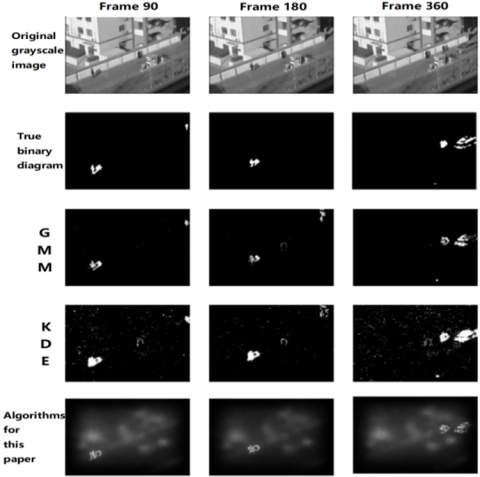
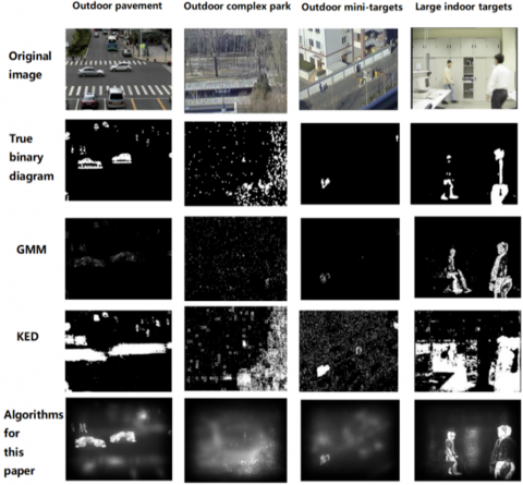
Figure 11. Comparative analysis of different algorithms
The illustrations follow a sequence wherein the initial row displays frames of original images from diverse environments: outdoor roads, intricate outdoor parks, minuscule outdoor objects, and sizable indoor entities. The ensuing row showcases authentic binary images. The Gaussian Mixture Model (GMM) derived segmentation results, constituting the third row, exhibit significant omissions. The fourth row, which employs the Kernel Density Estimation (KDE), manifests certain false detections. The final row amalgamates the GBVS algorithm with the HS algorithm, effectively suppressing noise while fully extracting the moving target. Comparative analysis suggests that this fusion yields results superior to the previously mentioned methods (Figure 11 and Figure 12).
Figure 12. Comparative analysis across varied scenarios
Figure 13. FPGA-based experimental outcomes
A hardware-infused parallel acceleration scheme for moving image detection has been proposed to enhance recognition efficiency and performance. To assess the efficacy of this system in moving image processing, a traditional CPU scheme is established as a benchmark for juxtaposition. The implementation specifics are as follows: OpenCV has been utilized to replicate the experimental algorithm on the PC platform, outfitted with a 12th Gen Intel (r) Core (TM) i7-12700h, operating at a frequency of 2.30 GHz. It is noteworthy that during the programming phase, parallel acceleration processing was eschewed, and OpenCV's pertinent functions were invoked to instantiate the inter-frame difference algorithm. The outcomes are illustrated in Figure 13.
Moving target detection, an integral facet of surveillance video systems, has been approached in this research to delineate moving targets from their backgrounds. This delineation aids subsequent operations, particularly in target detection within intricate backgrounds, and sets the stage for proficient target tracking. In the endeavour to detect saliency, priority was given to the extraction of pivotal information from images whilst concurrently filtering out superfluous data. Recognising the susceptibility of optical flow to various factors, leading to its potential instability, a moving target detection algorithm was postulated, amalgamating the optical flow technique with saliency detection.
A thorough investigation into the significance detection algorithm based on image GBVS was undertaken, culminating in the enhancement of the image fusion methodology. Comparative analysis, adjusting the weighted fusion weights, revealed commendable detection outcomes. MATLAB simulations facilitated a juxtaposition between traditional methodologies and the algorithm proposed herein, extending this comparison across diverse environments. It was discerned that the newly proposed methodology exhibited superior capabilities in isolating the complete moving target as opposed to traditional approaches.
In a subsequent evaluation, the frame rates of target detection, when accelerated by both PC and FPGA, were juxtaposed. Analyses illuminated that video disruptions, emanating from the lack of parallel acceleration on PCs, were expected. This resulted in suboptimal real-time performance. In stark contrast, FPGA's processing time was found to be negligible in comparison to the single-frame image transmission time, ensuring seamless and real-time video output. This marked enhancement in processing speed can be attributed to the FPGA hardware's prowess in accelerating parallel pipeline operations within image processing. Certain processes were completed in mere nanoseconds, a feat unattainable by CPU-based PC serial processing platforms.
Concerning video stream transmission, the adoption of the AXI bus transmission was noted, with the AXI data transmission segment leveraging the Xilinx official IP core. Despite achieving the desired functionality, it was observed that the code encapsulated by the official IP core was encumbered with redundancies—components not utilised within this experiment. These superfluous elements, while inactive, still consumed computational resources. Therefore, future endeavours could be channelled towards refining the system's performance by re-evaluating the foundational code of the AXI protocol, streamlining and repackaging it as necessary.
Fujian Provincial Youth Fund (Grant No.: 2022J05290); Exploration of multi-course integration mode under the background of new engineering and innovation and entrepreneurship (Grant No.: JG202210); The Transverse Subject of the Enterprise (Grant No.: ZK-HX22094).
[1] Poppe, R. (2010). A survey on vision-based human action recognition. Image and Vision Computing, 28(6): 976-990. https://doi.org/10.1016/j.imavis.2009.11.014
[2] Li, Y. (2016). Moving object detection in complex background. Department of Xi'an University of Technology, Xi'an, China.
[3] Abd, R.G., Ibrahim, A.W.S., Noor, A.A. (2023). Facial emotion recognition using HOG and convolution neural network. Ingénierie des Systèmes d’Information, 28(1): 169-174. https://doi.org/10.18280/isi.280118
[4] Bharathi, L., Chandrabose, S. (2022). Machine learning-based malware software detection based on adaptive gradient support vector regression. International Journal of Safety and Security Engineering, 12(1): 39-45. https://doi.org/10.18280/ijsse.120105
[5] Yazdi, M., Bouwmans, T. (2018). New trends on moving object detection in video images captured by a moving camera: A survey. Computer Science Review, 28: 157-177. https://doi.org/10.1016/j.cosrev.2018.03.001
[6] Wang, G., Kou, H., Li, T. (2011). A multi-modal fusion news video item segmentation algorithm. Computer Engineering and Science, 33(6): 46-50.
[7] Li, C.M., Bai, H.Y., Guo, H.W., Liang, H.J. (2018). Moving object detection and tracking based on improved optical flow method. Chinese Journal of Scientific Instrument, 39(5): 249-256.
[8] Stauffer, C., Grimson, W.E.L. (1999). Adaptive background mixture models for real-time tracking. In Proceedings. 1999 IEEE Computer Society Conference on Computer Vision and Pattern Recognition, Fort Collins, CO, USA, pp. 246-252. https://doi.org/10.1109/CVPR.1999.784637
[9] Sobral, A., Vacavant, A. (2014). A comprehensive review of background subtraction algorithms evaluated with synthetic and real videos. Computer Vision and Image Understanding, 122: 4-21. https://doi.org/10.1016/j.cviu.2013.12.005
[10] Gorelick, L., Blank, M., Shechtman, E., Irani, M., Basri, R. (2007). Actions as space-time shapes. IEEE Transactions on Pattern Analysis and Machine Intelligence, 29(12): 2247-2253. https://doi.org/10.1109/TPAMI.2007.70711
[11] Tsai, Y.H., Yang, M.H., Black, M.J. (2016). Video segmentation via object flow. In Proceedings of the IEEE Conference on Computer Vision and Pattern Recognition, Las Vegas, NV, USA, pp. 3899-3908. https://doi.org/10.1109/CVPR.2016.423
[12] Yu, H.F., Liu, W., Yuan, H., Zhao, H. (2017). Moving object detection based on sub-block motion compensation. Acta Electonica Sinica, 45(1): 173-180. https://doi.org/10.3969/j.issn.0372-2112.2017.01.024
[13] Huang, F. (2020). Research on moving target detection method in dynamic background with combination of optical flow and saliency. Department of Hunan Institute of Science and Technology, Hunan, China.
[14] Katopodis, V., Felipe, D., Tsokos, C., Groumas, P., Spyropoulou, M., Beretta, A., Kouloumentas, C. (2016). Multi-flow transmitter based on polarization and optical carrier management on optical polymers. IEEE Photonics Technology Letters, 28(11): 1169-1172. https://doi.org/10.1109/LPT.2016.2533663
[15] Guo, P.F., Jin, Q., Liu, W.J. (2023). Saliency detection via objectness foreground object and background prior. Computer Engineering & Science, 40(9): 1679-1688. https://doi.org/10.3969/j.issn.1007-130X.2018.09.021
[16] Li, W., Xu, D., Shi, J., Huang, S. (2022). Review of salient object detection research: Methods, applications and trends. Computer Application Research, 5(13): 1-11.
[17] Shi, Z. (2005). Intelligent science. Tsinghua University Publishing House, Beijing, China, 2005.
[18] Treisman, A.M., Gelade, G. (1980). A feature-integration theory of attention. Cognitive Psychology, 12(1): 97-136. https://doi.org/10.1016/0010-0285(80)90005-5
[19] Koch, C., Ullman, S. (1985). Shifts in selective visual attention: Towards the underlying neural circuitry. Human Neurobiology, 4(4): 219-227.
[20] Itti, L., Koch, C., Niebur, E. (1998). A model of saliency-based visual attention for rapid scene analysis. IEEE Transactions on Pattern Analysis and Machine Intelligence, 20(11): 1254-1259. https://doi.org/10.1109/34.730558
[21] Huang, H., Chen, J., Xue, H., Huang, Y., Zhao, T. (2018). Time-variant visual attention in 360-degree video playback. In 2018 IEEE International Symposium on Haptic, Audio and Visual Environments and Games (HAVE), Dalian, China, pp. 1-5. https://doi.org/10.1109/HAVE.2018.8547419
[22] Sun, H. (2016). Research on visual saliency detection algorithm based on multi-feature fusion. Department of Chongqing University, Chongqing, China.
[23] Christopoulos, C., Skodras, A., Ebrahimi, T. (2000). The JPEG2000 still image coding system: An overview. IEEE Transactions on Consumer Electronics, 46(4): 1103-1127. https://doi.org/10.1109/30.920468
[24] Nikitha, R., Vedhapriyavadhana, R., Anubala, V.P. (2018). Video saliency detection using weight based spatio-temporal features. In 2018 International Conference on Smart Systems and Inventive Technology (ICSSIT), Tirunelveli, India, pp. 343-347. https://doi.org/10.1109/ICSSIT.2018.8748400
[25] Farazi, M., Khan, S., Barnes, N. (2021). Question-agnostic attention for visual question answering. In 2020 25th International Conference on Pattern Recognition (ICPR), Milan, Italy, pp. 3542-3549. https://doi.org/10.1109/ICPR48806.2021.9413330
[26] Zhang, W., Tian, Y., Zha, X., Liu, H. (2016). Benchmarking state-of-the-art visual saliency models for image quality assessment. In 2016 IEEE International Conference on Acoustics, Speech and Signal Processing (ICASSP), Shanghai, China, pp. 1090-1094. https://doi.org/10.1109/ICASSP.2016.7471844
[27] Cui, L. (2016). Research on moving target tracking based on optical flow method. Department of Tianjin Polytechnic University, China.
[28] Song, H., Liu, Z., Du, H., Sun, G. (2016). Depth-aware saliency detection using discriminative saliency fusion. In 2016 IEEE International Conference on Acoustics, Speech and Signal Processing (ICASSP), Shanghai, China, pp. 1626-1630. https://doi.org/10.1109/ICASSP.2016.7471952
[29] Shi, J., Wang, J., Wang, H. (2008). Real-time detection method of human motion based on optical flow. Journal of Beijing University of Science and Technology, 28(9): 794-797.
[30] Fan, F., Ma, Y., Huang, J., Liu, Z. (2018). Infrared image enhancement based on saliency weight with adaptive threshold. In 2018 IEEE 3rd International Conference on Signal and Image Processing (ICSIP), Shenzhen, China, pp. 225-230. https://doi.org/10.1109/SIPROCESS.2018.8600468
[31] Gacsádi, A., Grava, C., Tiponut, V., Szolgay, P. (2006). A CNN implementation of the Horn & Schunck motion estimation method. In 2006 10th International Workshop on Cellular Neural Networks and Their Applications, Istanbul, Turkey, pp. 1-5. https://doi.org/10.1109/CNNA.2006.341615
[32] Wang, H. (2013). Vehicle abnormal behavior detection based on video. Department of Shenyang University of Technology, China.
[33] Gibson, J.J. (1950). Image motion and its use in vision. Psychological Review, 57(6): 354-371.
[34] Ren, Y., Wan, Y., Hu, B., Gong, C. (2016). Partial discharge monitoring and analysis of oil-immersed main transformer in wind farm based on UHF technology. Journal of Shanghai University of Science and Technology, 38(6): 540-545. https://doi.org/10.13255/j.cnki.jusst.2016.06.006
[35] Horn, B.K.P., Schunck, B.G. (1981). Determining optical flow. Artificial Intelligence, 17(1): 185-203.
[36] Huang, F., Yi, J., Wu, J. (2020). Moving object detection method based on the combination of optical flow method and saliency. Journal of Chengdu Institute of Technology, 23(1): 13-18.