Haidong Yang![]() | Renyong Guo*
| Renyong Guo*![]()
© 2023 IIETA. This article is published by IIETA and is licensed under the CC BY 4.0 license (http://creativecommons.org/licenses/by/4.0/).
OPEN ACCESS
The study of crowd movement and behavioral patterns typically relies on spatio-temporal localization data of pedestrians. While monocular cameras serve the purpose, industrial binocular cameras based on multi-view geometry offer heightened spatial accuracy. These cameras synchronize time through circuits and are calibrated for external parameters after fixing their relative positions. Yet, the flexibility and real-time adaptability of using two different cameras or smartphones in close proximity, forming a short-baseline binocular camera, presents challenges in camera time synchronization, external parameter calibration, and pedestrian feature matching. A method is introduced herein for jointly addressing these challenges. Images are abstracted into spatial-temporal point sets based on human head coordinates and frame numbers. Through point set registration, time synchronization and pedestrian matching are achieved concurrently, followed by the calibration of the short-baseline camera's external parameters. Numerical results from synthetic and real-world scenarios indicate the proposed model's capability in addressing the aforementioned fundamental challenges. With the sole reliance on crowd image data, devoid of external hardware, software, or manual calibrations, time synchronization precision reaches the sub-millisecond level, pedestrian matching averages a 92% accuracy rate, and the camera's external parameters align with the calibration board's precision. Ultimately, this research facilitates the self-calibration, automatic time synchronization, and pedestrian matching tasks for short-baseline camera assemblies observing crowds.
spatio-temporal localization, binocular cameras, multi-view geometry, short-baseline binocular camera, camera synchronization, external parameter calibration, pedestrian feature matching, spatial-temporal point sets, self-calibration
Locating individuals within densely populated crowds entails determining the spatio-temporal positions of a vast majority of people in such scenes. Primarily, these findings serve as a data source and empirical foundation for various industrial and research endeavors. They have been frequently utilized in the domains of safety management [1], pedestrian dynamics [2], and intelligent transportation [3], among others. Additionally, dense crowd positioning has emerged as one of the research themes in crowd behaviour analysis [4-8]. A myriad of sensors is available to gather pedestrian data. Upon evaluating factors such as data precision, equipment costs, and deployment costs, cameras are discerned to possess distinct advantages. The precision in extracting crowd-related features through computer vision (CV) methods has been notably enhanced under the influence of deep learning [9-11]. Furthermore, the implementation of binocular stereoscopic vision (BSV) with multiple cameras to execute spatial triangulation [12] has the potential to ameliorate positioning accuracy and spatial dimensions. While a multitude of industrial binocular cameras can accomplish data collection tasks for short-baseline stereoscopic vision, an even more favourable approach entails the ad-hoc pairing of two standard cameras or smartphones to form a short-baseline camera assembly. Such combinations permit swift execution of controlled and natural experiments. However, in comparison to industrial binocular cameras, this freely-formed camera assembly confronts three pivotal challenges when observing from multiple angles: precise time synchronization, manual external camera parameter calibration, and pedestrian matching across multiple views. Hence, this study pivots its attention towards jointly addressing these three challenges, striving to propose a method that balances both engineering practicality and theoretical significance.
These three pivotal challenges can be distilled into the geometric object correspondence issues enumerated in Table 1. An intuitive approach to resolve these correspondence issues involves transitioning from static image resolution to dynamic scene resolution. Features of pedestrians are first extracted using detectors [9, 10, 13]. Following video frame time alignment [14, 15] and after the camera assembly calibration is completed [16], triangulation is performed on each pair of video frames [12, 17].
However, what appears intuitively feasible often comes with intricacies. Assuming the exclusive use of image data without relying on camera hardware/software control and manual calibration, resolving the aforementioned relationships becomes reminiscent of the chicken-or-the-egg conundrum. The underlying reason lies in the inter-dependencies that exist among C1~C3. Existing research purely based on images [15, 18-21] either does not achieve the temporal precision required by BSV or relies on features unsuitable for crowd scenes characterized by significant occlusions. Furthermore, when C3 is unknown or fraught with large errors [22], C1 and C2 become indefinable. Only a handful of research endeavors have proposed joint solutions for C2 and C3 when dealing with individual pedestrians [23]. The presented research intends to circumvent these challenges through an innovative approach.
Table 1. Point set correspondence
|
Serial No. |
Name |
Point Set Relationship |
Function |
|
C1 |
Feature point matching |
Point-point relationship |
Correspondence of pedestrian features in left and right views |
|
C2 |
Fundamental matrix estimation |
Point-line relationship |
Correspondence of points and lines between left and right views or rigid transformations of coordinate systems |
|
C3 |
Time synchronization |
Point-set relationship |
Temporal correspondence between left and right view videos |
Figure 1. Point sets with correspondence in left and right views
The following perspectives are proposed in this study:
The precise methodology encompasses both models and their respective solution algorithms. As depicted in Figure 1, head points from both views, along with time, are abstracted as point sets in a linear space, with the time axis orthogonal to the imaging plane. Subsequently, the correspondence issues of C1-C3 are recast into the challenge of solving point set stitching problems [24, 25]. The specific solution algorithm is then tailored according to the uniqueness of the problem.
Main contributions of this study are:
Prerequisites for the introduced method encapsulate two dimensions: the known internal parameters of the cameras and the assumption that the scene entails a crowd walking on an approximate plane. These conditions, while being easily achievable in experimental or production settings, resonate with real-world applications.
In subsequent sections, works overlapping with the research objectives of this study are introduced. Their distinct characteristics, strengths, and limitations, when applied to dense crowd positioning, are briefly discussed. The foundational knowledge section provides the theoretical bases on which the core algorithms of this study hinge, specifically the theory related to the Iterative Closest Point (ICP) algorithm.
2.1 Related studies
This segment introduces works congruent with the topics addressed in this study, serving as the foundational base for this research. Comparisons between the present study and existing literatures are further elaborated in Sections 4.1 and 4.2.
Time synchronization emerges as a prerequisite for data fusion from multiple cameras. A plethora of studies have utilized supplementary software and hardware tools during data acquisition to achieve optimal time accuracy. Among them, Smid and Matas [26] deployed camera flash as a synchronization tool. Faizullin et al. [27] utilized a gyroscope for synchronizing smartphones with commercial depth cameras. Work by Ansari et al. [28] enabled multiple Android phones to capture synchronously with sub-millisecond precision, largely leaning on network communication from camera capture software, albeit with high inter-camera dependencies. In the realms of video archive retrieval and alignment, studies [29, 30] have achieved large-scale spatial-temporal alignment through video features and spatio-temporal encoding. Common video processing tasks often employ methods by Wang et al. [15] for non-linear time alignment, necessitating manual and software interaction. Sinha's series of works [31, 32] utilize the tangent of imaging silhouettes of individual pedestrians to determine the fundamental matrix, subsequently deploying the Ransac algorithm to compute time offset from numerous matches. However, this method is found inadequate for long-distance observations of dense crowds. Takahashi et al. [33] synchronized time and calibrated multiple cameras for posture recognition using human body key points. Their model, an optimization problem with constraints, was deemed ill-suited for crowds with extensive obstructions. Numerous other studies [14, 18, 34], although capable of resolving time offset, presume the fundamental matrix as a given condition. Yet, Albl et al. [23], who employed pedestrian trajectories, introduced a method to jointly address time offset and the fundamental matrix, despite the challenges associated with automatically obtaining high-quality trajectories in dense crowds.
Pedestrian feature matching holds significant weight in multi-view pedestrian positioning research. Common pedestrian positioning methods are categorized into instance-level and pixel-level [35], both contingent upon pre-known time offsets and scene geometry. The pixel-level, or pseudo radar method [36], is predicated on depth mapping for 3D detection and remains ineffectual for dense crowds. Instance-level pedestrian positioning mandates object feature matching followed by positioning of object instances. The study by Li et al. [37], termed stereoscopic R-CNN and purposed for autonomous driving, employed corresponding patches from left and right views during training to generate features, facilitating simultaneous detection and association during prediction. Qin et al. [38] made use of a series of hypothetical 3D candidate anchor points for foreground object detection. At this juncture, the matching relationship of the ROI in the left and right views is assumed known. While their triangulation accuracy and match quality are commendable, further refinements are required for pedestrian or crowd research. Bertoni et al. [35], by training on human key points, deployed both left and right view key points and Reid method for pedestrian matching. However, in scenarios with considerable occlusions, their key point detector fails. Pon et al. [39] used metrics formed from the mean and variance of pixel intensity values within the ROI for matching in left and right views, yet its applicability for dense crowd scenarios remains unverified.
Fundamental matrix estimation, pivotal for 3D object positioning in space, ranks among the central issues in multi-view geometry [12, 17]. The short-baseline triangulation explored in this study necessitates sub-pixel precision. Numerous sub-pixel object relation refinement studies exist [40, 41], but these algorithms come with high operational costs. There's also a wealth of studies on outlier pruning [42], most of which are similarly resource-intensive. This study plans to deploy the lightweight random algorithm, GraphCut [43], for estimating the fundamental matrix.
2.2 Preliminary knowledge
This section introduces the foundational concepts and provides a broad description of the models and algorithms utilized in the study. The challenges are re-framed as point set registration problems, solution for which is commonly termed as the ICP algorithm. While this method is typically applied to static physical space for point set registration, in this context, it us adapted for alignment within image spaces and time.
Matrix optimization knowledge is pivotal for understanding the models and algorithms presented. Du et al. [25] provided a special form of Lemma 2, which has been generalized in this study. Throughout the proofs of the lemmas and theorems in this work, the Frobenius norm $\|\cdot\|_F$ of matrices and the Trace(·) function are repeatedly employed. For detailed definitions and properties, please refer to the study [44]. Relevant lemmas related to this study are presented below.
Lemma 1. Given two m-dimensional point sets $\left\{q_i\right\}_{i=1}^{N_p}$ and $\left\{p_i\right\}_{i=1}^{N_p}$, the function $F(t)=\sum_{i=1}^{N_p}\left\|q_i+t-n_i\right\|_2^2$ achieves its minimum when $t=\frac{1}{N_p} \sum_{i=1}^{N_p}\left(n_i-q_i\right)$.
Lemma 2. For given matrices $A \in \mathbb{R}^{m \times m}$, $B \in \mathbb{R}^{m \times N_p}$, $C \in \mathbb{R}^{m \times N_p}$, $t \in \mathbb{R}^m$, and $J=(1, \cdots, 1)^T \in \mathbb{R}^{N_p}$, set D=B-C, A is invertible, then the point of minimum value for matrix function $L(t)=\left\|A\left(B+t J^T-C\right)\right\|_F$ is:
$t^*=-\frac{1}{N_p} D J=-\frac{1}{N_p} \sum_{i=1}^{N_p}\left(B_i-C_i\right)$.
Typical transformations for point set registration can be categorized into rigid transformations, non-rigid transformations, affine and projective transformations, or even further advanced non-linear transformations. Existing literatures [24, 25, 45] have already detailed analytical and proof-based discussions on the related data theories. Most relevant to this work are the models based on rigid transformations, which will be further modified. The model is defined as:
$\begin{array}{cc}\underset{X, t, j \in\left\{1,2, \ldots, N_m\right\}}{\operatorname{argmin}} & \left(\sum_{i=1}^{N_p}\left\|\left(X p_i+t\right)-m_j\right\|_2^2\right) \\ \text { s.t. } & X^T X=I, \operatorname{det}(X)=1\end{array}$ (1)
where, $p_i, m_i \in \mathbb{R}^3$ and $X_2 \in \mathbb{R}^2 \times \mathbb{R}^2$. The conventional approach to solving the rigid transformation model using the ICP algorithm is as follows:
Step 1. Determine the correspondence under current parameters.
$\begin{aligned} & c_k(i)=\underset{j \in\left\{1,2, \ldots, N_m\right\}}{\operatorname{argmin}}\left(\left\|\left(X_{k-1} p_i+t_{k-1}\right)-m_j\right\|_2^2\right), \\ & i=1, \ldots, N_p .\end{aligned}$
Step 2. Based on the current correspondence, new parameters are computed.
$\begin{array}{cc}\left(X_k, t_k\right)=\underset{X, t}{\operatorname{argmin}} & \left\|X A+J t^T-B\right\|_F^2, \\ \text { s.t. } & X^T X=I, \operatorname{det}(X)=1,\end{array}$ (2)
Step 3. If convergence criteria are not met, return to Step 1.
In Eq. (2), $J=(1, \ldots, 1)^T$ represents a column vector with $N_p$ dimensions, $A \in \mathbb{R}^{3 \times N_p}$ its column vectors are $p_i$, $B \in \mathbb{R}^{3 \times N_p}$, and its column vectors are $m_j$.
In this section, methods for addressing problems C1~C3 under the short-baseline camera combination will be elucidated. Initially, an overview of the dense crowd 3D positioning process is presented, with clarity provided regarding the position of the research discussed within this broader process. Subsequently, based on the viewpoints proposed in the prologue, pertinent models are introduced. Finally, solution algorithms for these models are described, underpinned by pertinent mathematical theories, for which corresponding proofs are provided.
Referring to Figure 2, the comprehensive process for dense crowd 3D positioning is outlined. Here, $V_l=\left\{I_i\right\}$ and $V_r=\left\{I_j\right\}$ denote video sequences, $H_l, H_r \subset \mathbb{R}^{\mathbb{3}}$ are respectively the point sets composed of image coordinates of pedestrian heads in left and right views an time values. $P_{s t}$ symbolizes a set of parameters, encompassing time offsets, external camera parameters, and transformations employed for pedestrian matching. Four segments are represented in the figure, with the third segment, temporal-spatial parameter estimation, and the dark rounded rectangle in the fourth segment correlating directly with the primary focus of this research. Green and blue arrows, respectively, represent data pertinent to the left and right views.
Figure 2. Overall process of pedestrian positioning
The tasks associated with parameter estimation and feature matching between the left and right views in the aforementioned process are addressed within this study.
3.1 Problem definition
The temporal-spatial parameter estimation process is simplified here as a point set matching model. Upon inputting the left and right view image sequences $V_l$ and $V_r$ into the pedestrian head detection module, point sets $H_l$ and $H_r$ on $\mathbb{R}^3$ are obtained respectively. Assuming $p_i \in H_l, m_j \in H_r$, to jointly solve problems C1~C3, the following objectives are defined:
The rigid transformation model presented in Eq. (1) is deemed unsuitable for this context and necessitates the following adaptations:
$\begin{array}{cl}\underset{X, t, j \in\left\{1,2, \ldots, N_m\right\}}{\operatorname{argmin}} & \left(\sum_{i=1}^{N_p}\left\|\left(X p_i+t\right)-m_j\right\|_2^2\right) \\ & X^T X=I, \operatorname{det}(X)=1, \\ \text { s.t. } & X=\left[\begin{array}{cc}X_2 & 0 \\ 0 & 1\end{array}\right] .\end{array}$ (3)
where, $p_i, m_i \in \mathbb{R}^3$, $X_2 \in \mathbb{R}^2 \times \mathbb{R}^2$.
Newly incorporated conditions reduce the degree of freedom in the transformation, permitting only rotation around time. Shuster [46] parametrized such rotation matrices by a unit vector in space μ and the angle of rotation α around it, as shown:
$\operatorname{Rot}(\alpha, \mu)=I_3+\sin (\alpha)[\mu]_{\times}+(1-\cos (\alpha))[\mu]_{\times}^2$ (4)
where, $[\mu]_{\times} \in \mathbb{R}^{3 \times 3}$ is an anti-symmetric matrix, denoted as the cross product matrix with respect to μ. If $\forall v \in \mathbb{R}$, then there is $\mu \times v=[\mu]_{\times} v$; assuming $\mu=\left(\mu_1, \mu_2, \mu_3\right)^T$, then $[\mu]_\times$ is defined as:
$[\mu]_{\times}=\left[\begin{array}{ccc}0 & -\mu_3 & \mu_2 \\ \mu_3 & 0 & -\mu_1 \\ -\mu_2 & \mu_1 & 0\end{array}\right]$
Thus, in the short-baseline scenario, only the rotation axis $\mu_0$ is known as a vector $(0,0,1)^T$, while the rotation angle $\alpha$ remains an estimated parameter. Here, the objective function in Eq. (3) is defined and is reformulated as follows:
$\begin{gathered} \left(X_k, t_k\right)=\underset{X, t}{\operatorname{argmin}} \mathrm{L}(X, t) \\ \text { s.t. } \quad X=\operatorname{Rot}\left(\alpha, \mu_0\right), \end{gathered}$
where $\quad \mathrm{L}(X, t)=\left\|X A+t J^T-B\right\|_F^2$. (5)
Upon defining the model, the iterative process discussed in Section 2.2 can be employed for solutions. The subsequent sections provide analytical solutions for single-step iterations.
3.2 Single-step analytical solution
The single-step solution method for Eq. (5) during iteration significantly differs from the solution method for Eq. (2). Herein, an analytical solution for a single step iteration of Eq. (5) is provided. Corollary 1 is a generalized form of Lemma 1 and will also be used in Eq. (2). The proofs for propositions and theorems are presented in the appendix.
Corollary 1. Let matrices be given as $X \in \mathbb{R}^{m \times m}$, $A \in \mathbb{R}^{m \times m}$, $B \in \mathbb{R}^{m \times N_p}$, $C \in \mathbb{R}^{m \times N_p}$, $t \in \mathbb{R}^{m \times 1}$, $J=(1, \cdots, 1)^T \in \mathbb{R}^{N_p}$, with $B_i$ and $C_i$ being column vectors of B and C respectively. Define functions $\mathrm{L}_1(X, t)$ and $\mathrm{L}_2(X)$ as follows:
$\begin{aligned} \mathrm{L}_1(X, t) & =\left\|A\left(X B+t J^T-C\right)\right\|_F^2 \\ \mathrm{~L}_2(X) & =\|A(X \tilde{B}-\tilde{C})\|_F^2\end{aligned}$
where, $J=(1, \ldots, 1)^T$ is a $N_p$-dimensional vector, and both $\tilde{B}=B-\frac{1}{N_p}\left(\sum_{i=1}^{N_p} B_i\right) J^T$ and $\tilde{C}=C-\frac{1}{N_p}\left(\sum_{i=1}^{N_p} C_i\right) J^T$ hold. Then, the optimal solution $X^*$ for $\mathrm{L}_2(X)$ is the optimal solution of $\mathrm{L}_{1(X, t)}$ with respect to $\mathrm{X}$, and the optimal solution of $\mathrm{L}_1(X, t)$ with respect to $t$ is:
$\begin{aligned} t^* & =-\frac{1}{N_p} \sum_{i=1}^{N_p}\left(X^* B_i-C_i\right), \\ Y^* & =X^* .\end{aligned}$
Theorem 1. Given matrices $A, B \in \mathbb{R}^{3 \times N_p}$, $B \in \mathbb{R}^{3 \times N_p}$, and $\mu_0=(0,0,1)^T$, the minimum value of function
$\mathrm{L}(\alpha)=\left\|\operatorname{Rot}\left(\alpha, \mu_0\right) \tilde{A}-\tilde{B}\right\|_F^2$
appears at:
$\alpha^*=\operatorname{argmax}\left(\mathrm{L}_2\left(\arctan \frac{-d 1}{d_2}\right), L_2\left(\arctan \frac{-d 1}{d_2}+\pi\right)\right)$,
where, $d_1=C_{12}-C_{21}$ and $d_2=-\left(C_{11}+C_{22}\right) ; C_{i j}$ are the respective elements at the corresponding positions of $C=$ $\tilde{A} \tilde{B}^T$, and $\mathrm{L}_2(\alpha)=d_1 \sin \alpha+d_2(1-\cos \alpha)$.
3.3 Algorithm
The algorithm consists of two parts: the point set alignment and the fundamental matrix estimation. The point set alignment is further divided into the FeatureMatching process, the RansacRegistration denoising process, and the TransformEstimationFine refinement process. Detailed descriptions follow, along with pseudocode implementations of the primary processes.
|
Algorithm 1 TwoViewAlignmentST |
|
Procedure TwoViewAlgMain $\left(H_l, H_r\right)$ $k d t r e e_r \leftarrow$ GenerateKdtree $\left(H_r\right)$ $\operatorname{corres}_{i j} \leftarrow$ FeatureMatching $\left(H_l, H_r\right)$ $X_{k-1}, t_{k-1} \leftarrow$ RansacRegistration $\left(\right.$corres $\left._{i j}, H_l, H_r\right)$ While $($relerr $($fitness$)<1 e-6$ or loop $<100)$ $H_l \leftarrow X_{k-1} H_l+t_{k-1}$ $c_{k i} \leftarrow$ Get corresponding indexes of $H_l$ in $kdtree_r$ $\left(X_k, t_k\right) \leftarrow$ TransformEstimation $\left(H_l, H_r, c_{k i}\right)$ computing fitness and loop EndWhile $\left(X_k, t_k\right) \leftarrow$ TransformEstimationFine$\left(H_l, H_r, c_{k i}\right)$ computing fitness and loop Return $X_k, t_k, c_{k i}$, fitness |
3.3.1 Point set alignment algorithm
The FeatureMatching process employs point cloud feature methods to calculate the correspondence between the point sets $H_l$ and $H_r$ of the left and right views, and apply filtering. At this stage, the point sets of the left and right views appear remarkably similar in visual representation, but their positions and angles do not coincide. Point cloud feature extraction algorithms, as described in the studies [47, 48], can be used to find corresponding points between point sets. However, many erroneous matches may occur. Initially, forward and reverse matching must be conducted and mutually validated. Next, matches are grouped and counted based on their temporal offset, allowing for the selection of groups within a specified time deviation range.
The RansacRegistration process employs the relationships identified from point set feature matching to extract an initial solution using the Ransac algorithm. Implementation details of the Ransac algorithm are not presented in this text; readers are directed to Schnabel's literature [49] for details.
The TransformEstimationFine process provides an analytical solution for Eq. (2) in Step 2 based on the specifics of the short baseline scenario. Traditional rigid transformation estimations [24, 45] require the calculation of 3 degrees of freedom. However, due to the distinct characteristics of the short-baseline scenario, the transformation degree of freedom in model Eq. (4) is reduced to 1. The single-step analytical solution during the iteration process was previously proven in Section 2.2. According to Proposition 1, the optimal value of Xk can be calculated first, and then tk can be calculated through Xk.
The pseudocode implementation of the aforementioned tasks is represented as Algorithm 1 (TwoViewAlignmentST).
3.3.2 Fundamental matrix estimation algorithm
Estimation of scene geometry (Problem C2) requires both temporal synchronization and sub-pixel matching precision as prerequisites. With temporal synchronization already achieved, two methods can address the sub-pixel synchronization challenge. One approach involves the utilization of corresponding point refinement algorithms [50, 51], while the other aims to increase the number of matching points, subsequently filtering a small subset that possesses sub-pixel precision. Both methods will be harnessed in this work.
The Asift feature descriptor [52] is used to enhance the sample volume. Its fundamental principle involves performing multi-perspective affine transformations on images and then employing descriptors like Sift, Orb, Brisk, etc., to extract features exhibiting affine invariance. One of the advantages of the Sift feature descriptor is the extraction of key points with exceptional sub-pixel properties. Therefore, by combining the Asift and Sift algorithms, an increase in the number of matching point samples is achieved, all the while preserving sub-pixel correspondence. Eventually, Graphcut [43] is employed to discard matches that don't possess sub-pixel precision.
This section aims to validate the model and algorithm in terms of principles and applicability, corresponding respectively to Sections 4.1 and 4.2. The objective of the principle validation is to assess the algorithm's performance on synthetic data ground truth and when quantifiable noise is introduced. This ensures the upper limit of its convergence accuracy is confirmed, and the interval of its location error is analyzed. The objective of applicability validation, as detailed in Section 4.2, is to use complex crowd scenes to validate issues C1 and C2. The adaptability of the algorithm to different pedestrian head detectors and its performance under varying overlap degrees between left and right views is also explored.
4.1 Synthetic data validation
Synthetic data experiments utilized the STCrowd [53] dataset, collected using LIDAR and cameras and annotated manually. This resulted in the generation of 2D projection data on the pixel plane. The pedestrian head images in this dataset underwent a blurring process. To ensure accuracy, only LIDAR data was employed. Annotated point cloud 3D boxes were projected onto virtual cameras at different baseline distances and rotation angles to obtain the synthetic data. Subsequently, the algorithm's performance on multiple data sets for issues C1~C3 was assessed.
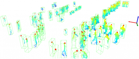
As shown in Figure 3, the highest point in each point cloud annotation was extracted as the pedestrian head point, denoted in red. This set is denoted as $H_{3 d}$. Projections of $H_{3 d}$ were then generated onto the pixel plane. The resolution and intrinsic parameter matrix of the camera were consistent with the equipment used in STCrowd [53]. Fifteen virtual camera sets were produced, with baseline lengths ranging from 0.06m to 0.2m, and rotation angles linearly proportional to baseline distances. After projection, 15 sets of projection point sets and under different external parameters were obtained. To validate algorithm reliability, a 1/5 duration of data from the left view was extracted while the entire right view was retained. The point sets of the left and right views $H_{l_i}$ and $H_{r_i}$ were then verified using the short baseline algorithm, TwoViewAlignmentST.
The point set alignment results are shown in Figure 4. The first column displays the point sets of the left and right views, with the left view's time range being a subset of the right view. The second column presents the aligned point clouds, and the third column indicates the position of a frame of the left view's point cloud in image space.
Figure 3. Point cloud in a crowd scene, with red dots representing pedestrian head points
Figure 4. Point set alignment and pedestrian matching results
4.1.1 Point set alignment and pedestrian matching results
Figure 5 presents numerical results under 15 different external parameters. It's evident that point set matching was successful, with the worst fitness of point sets (fitness_pt) being 88% and the best fitness being 98%. The accuracy rate of pedestrian matching (fitness_pid) also reached a similar level, indicating the algorithm's suitability for addressing the pedestrian matching issue.
Furthermore, in terms of the root mean square error (RMSE) of matching points (inliner_rmse), good results were also achieved. The maximum inliner RMSE was 5.5px, ensuring convergence even with a Gaussian noise of 10px when observing pedestrians within 20m, and this is a necessary condition for using the pedestrian head point detection tool.
4.1.2 Results of time synchronization
In these experiments, the time synchronization accuracy for all baselines was maintained at a frame level, implying that the accuracy achieved matches the time precision of the lidar used in the STCrowd dataset. With an image localization error of 5px, the algorithm was found to be suitable for addressing the C3 problem, which pertains to time synchronization.
4.1.3 Results and error analysis of external parameter estimation
Firstly, the influence of noise addition to feature points on triangulation localization after scene geometry recovery was explored. The results from Figure 6 indicate that to recover a usable fundamental matrix, pixel error must be kept below 0.2px, and the baseline distance must exceed 0.1m to achieve an effect consistent with standard industrial stereo cameras, wherein the accuracy is 9% at 15m and 1% at 0.5m.
Figure 5. Fit degree of point cloud stitching and RMSE of inliner matches
Figure 6. Mean of location errors and mean of error per meter
Figure 7. Isolines of pedestrian head positioning. a - Isolines of mean error in pedestrian head positioning; b - Isolines of error per meter in pedestrian head positioning
Furthermore, the impact of noise added to feature points on the accuracy of localization was discussed in case that the geometry of the scene is known. As can be discerned from Figure 7, to achieve a 5% accuracy in spatial triangulation, the pixel error must not exceed 0.2px. To ensure the triangulation accuracy reaches 0.2, the baseline distance must be greater than 0.08m and the pixel noise should not surpass 0.1px. In Figure 7(a), the presented results pertain to the mean of location errors, while in Figure 7(b), the results represent the mean of error per meter.
Based on the aforementioned numerical results, the viable range for pixel precision was determined. Additionally, it was concluded that directly using the pedestrian's head feature points to restore the fundamental matrix is infeasible.
4.2 Verification in real-world scenarios
The proprietary dataset, ZEDPed, was employed for verification purposes. As depicted in Figure 8, the lighting conditions were suboptimal, and there was significant obstruction of pedestrians. The data was captured using the ZED Mini stereo camera. Its circuit-level synchronized rolling shutter ensures high precision time synchronization between the left and right cameras, thereby providing an accurate reference for temporal alignment. The effective detection range stood at 15 meters, and the video lasted 30 seconds, totalling 300 frames.
Figure 8. Matching results with a 15-frame difference
Figure 9. Point cloud stitching results generated by manual annotation and various detectors. a — Results from manual annotation, b — Results from headhunter detector, c — Results from IIM detector, d — Results from P2P detector
Figure 10. Curves of stitching results from various detectors
Figure 11. Distribution of head points in 3D space and the impact of estimated external parameters on positioning accuracy
Given the data now available from the left and right camera videos, along with the internal parameters of the cameras, the ultimate output is the transformation between point sets. Initial steps involved the extraction of head points using head detectors like Headhunter [10], P2P [9], and IIM [54]. Following this, algorithms were employed to match head point sets $H_l$ and $H_r$ from both left and right views. Additionally, manual annotations of head points were done for all video frames in the ZEDPed dataset, without any trajectory matching or left-right view matching. In the following discussions, these annotations are referred to as "Anno".
Initially, the convergence and time synchronization accuracy of the algorithm at different time range overlap rates were addressed. Precision in pedestrian matching was not discussed due to the absence of a ground truth. Subsequently, the positioning accuracy of triangulation was presented.
4.2.1 Point set alignment results
Discussion will now focus on the algorithm's convergence results at different time overlap rates. Numerical results indicate that the algorithm can converge for both noisy detection results and manual annotations.
Head detectors, including Headhunter [10], P2P [9], and IIM [54], were employed to analyze the video, yielding three distinct sets of head point $H_l$ and $H_r$ data. Manual annotation data were also examined. Each point set $H_l$ was divided based on a time proportion, ranging from 10% to 100%, resulting in ten sets for the left view. These were then matched with their respective $H_r$. Figures 9(a), 9(b), 9(c), and 9(d) display the results corresponding to manual annotations and three detection tools at an overlap rate of 20%. In the illustrations, blue points represent matched points from the left view, light blue indicates unmatched points from the left view, and red signifies points from the right view.
Numerical outcomes suggest that the algorithm can converge at most time overlap degrees. Evaluation metrics employed were point set fitting and RMSE of the stitched matched points. Figures 10(a) and 10(b) display numerical curves for various detectors and overlap rates, representing fitting, inliner RMSE, and time synchronization accuracy. The findings are as follows:
4.2.2 Time synchronization results
Time synchronization accuracy varies significantly between detectors. Figure 10(c) presents accuracy for different detector-overlap rate combinations. Detailed results are:
4.2.3 External parameter estimation results
This section contrasts the impact of true and estimated extrinsic parameters on pedestrian positioning. The ground truth for the fundamental matrix was obtained from a calibration board, while its estimated value is derived using the fundamental matrix estimation method proposed in Section 3.3.2. Numerical results demonstrate that the employed algorithm achieves accuracy comparable to the calibration board.
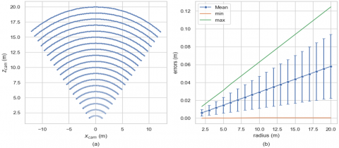
Initially, spatial point coordinates were generated in line with the camera's FOV (Field of View), resulting in the spatial fan-shaped point set shown in Figure 11 (a). Projections were subsequently created using the true internal and external camera parameters. The estimated external parameter values were finally utilized to recover spatial coordinates, which were then compared to produce the errors at various distances shown in Figure 11 (b). Figure 11 (b) presents the mean, standard deviation, and range of the triangulation errors.
An observable linear relationship exists between precision and the distance of space points from the camera. At 20m distance from the camera, the mean error was 0.06m, with the maximum error being 0.12m. This precision significantly surpasses the 9% accuracy at 20m of the depth map produced by standard stereo cameras. In practical applications, sub-pixel refinement of detected head points was conducted to achieve this level of precision.
4.3 Comparison with related works
For crowd data extraction, existing studies have primarily focused on positioning in the imaging plane [1], with business objectives centred around crowd behaviour analysis, crowd counting, and density estimation [55, 56]. Due to misidentifications caused by obstructions and high density in crowd scenarios, and combined with the three problems C1~C3, the complexity has been raised, and no research currently addresses all three problems simultaneously.
Numerous studies have sought to simultaneously solve time synchronization and scene geometry [14, 23, 32, 33, 57, 58]. However, these methods are not applicable in crowd scenarios. The primary reasons include their suitability only for scenes with individual or few unobstructed pedestrians and the inability of even the best trackers to obtain high-quality continuous trajectories in crowds. Moreover, the computational cost of determining correspondence between multi-view trajectories remains high.
Table 2. Pixel error requirements and time synchronization errors of different time synchronization methods
|
Method |
Average Frame Offset |
Average Time Offset |
Pixel Error |
Scene and Data |
|
Image Feature [32] |
0.2 frames |
6ms |
0.25px |
Single person, multiple datasets |
|
Image Feature [33] |
0.6 frames |
10ms |
3px |
Single person, single dataset |
|
Image Feature [23] |
1 frame |
67ms(estimated) |
Unknown |
Single person, multiple datasets |
|
Image Feature [14] |
0.35 frames |
8ms(estimated) |
2px~8px |
Single target, multiple datasets |
|
Flash [26] |
0.1frames |
3ms |
- |
Multi-person hockey game |
|
IMU & Circuit Trigger [27] |
- |
0.1ms |
- |
Android phone synchronized with depth camera |
|
NTP algorithm and Android API [28] |
- |
0.03ms |
- |
Multiple Android phones |
|
Image Feature [text] |
0.01frames |
0.7ms |
5px |
Congested crowd, single dataset |
|
Synthetic Data [text] |
0 frame |
0ms |
5px |
Congested crowd, multiple dataset |
Table 2 provides a comparison in terms of time accuracy, encompassing work similar to this study as well as methods that use circuit synchronization, gyroscopes, and other auxiliary software and hardware tools during video collection [26-28]. Experimental data indicate that the results of this study surpass image data-driven methods by an order of magnitude. While not exclusively due to the algorithm, it can be confirmed that the methodology achieves the level of true inter-camera time offset. Its advantage lies in not requiring additional software or hardware, and it remains effective even in densely crowded scenes with significant obstructions.
It cannot be numerically compared with feature matching because existing studies [35, 37, 39, 59] only provide algorithms in the matching process without giving corresponding numerical results. A comparison of constraints and properties is presented below:
In terms of scene geometry estimation, the method proposed herein achieves the precision of calibration board. Ortiz et al. [60] conducted an in-depth analysis of the positioning error of the ZED camera. Corresponding to the ZEDPED dataset with a resolution of 2208*1242, the mean μ and standard deviation σ are 0.17m and 0.14m respectively. From the results in Figure 11, the worst mean and standard deviation obtained are 0.06m and 0.065m, respectively. Hence, the fundamental matrix calculated by this method fully meets the precision requirements when observing pedestrians with short-baseline cameras.
Through the validation of models and algorithms using crowd scene instance data, the dilemma of the chicken-and-egg sequence has been resolved, and the validity of the proposed perspectives has been confirmed. Currently, no related work has been identified that simultaneously addresses these three issues in dense crowd scenarios.
Methodologically, the initial problem was reduced to a point cloud registration issue, and a Euclidean model that redefines the inner product was introduced. Experiments with synthetic data demonstrated that the algorithm can converge when dealing with noisy data produced by detectors and manual annotations. In terms of time synchronization, owing to a vast amount of valid samples, experiments in two scenarios reached the true level of camera time deviations. For pedestrian matching, a lightweight single-point multi-view pedestrian matching method was introduced to reduce computational costs and the likelihood of mismatches. Regarding the external parameter estimation in scene geometry, the method exploited the high similarity of short-baseline images and the abundant features of dense crowds, achieving sub-pixel accuracy comparable to calibration board.
While these three problems were successfully addressed simultaneously, several aspects remain that warrant improvement, specifically:
Lemma 1. Given two sets of $m$-dimensional points $\left\{q_i\right\}_{i=1}^{N_p}$ and $\left\{p_i\right\}_{i=1}^{N_p}$, the function $F(t)=\sum_{i=1}^{N_p}\left\|q_i+t-n_i\right\|_2^2$ attains its minimum at $t=\frac{1}{N_p} \sum_{i=1}^{N_p}\left(n_i-q_i\right)$.
Proof: Clearly, the vector $t$ is the average of the displacement vectors between $\left\{q_i\right\}$ and $\left\{n_i\right\}$. $\blacksquare$
Lemma 2. For given matrices $A \in \mathbb{R}^{m \times m}, B \in \mathbb{R}^{m \times N_p}, C \in$ $\mathbb{R}^{m \times N_p}, t \in \mathbb{R}^m$, and $J=(1, \cdots, 1)^T \in \mathbb{R}^{N_p}$. Let $D=B-C$, where $A$ is invertible. The point of minimum for the matrix function $\mathrm{L}(t)=\left\|A\left(B+t J^T-C\right)\right\|_F$ is
$t^*=-\frac{1}{N_p} D J=-\frac{1}{N_p} \sum_{i=1}^{N_p}\left(B_i-C_i\right)$
Proof:
$\begin{aligned} \mathrm{L}(t) & =\operatorname{tr}\left(\left(A D+A t J^T\right)^T\left(A D+A t J^T\right)\right) \\ & =\operatorname{tr}\left(D^T A^T A D+D^T A^T A t J^T+J t^T A^T A D+J t^T A^T A t J^T\right) .\end{aligned}$
Let $\mathrm{L}_1(t)=2 \operatorname{tr}\left(D^T A^T A t J^T\right)+\operatorname{tr}\left(J t^T A^T A t J^T\right)$. By properties of the trace of matrices,
$\mathrm{L}_1(t)=2 \operatorname{tr}\left(J^T D^T A^T A t\right)+\operatorname{tr}\left(J^T J t^T A^T A t\right)$.
It's clear that $\mathrm{L}_1(t)$ and $\mathrm{L}(t)$ share the same points of extremum.
Using the properties of matrix functions and the trace, the gradient of $\mathrm{L}_1(t)$ is
$\nabla_t \mathrm{~L}_1=2 A^T A D J+2 N_P A^T A t$.
Since $\mathrm{L}_1(t)$ is a convex function, it has its optimal solution when $\nabla_t \mathrm{~L}_1=0$:
$t^*=-\frac{1}{N_p} D J$. $\blacksquare$
Corollary 1. Let the matrices $X \in \mathbb{R}^{m \times m}, A \in \mathbb{R}^{m \times m}, B \in$ $\mathbb{R}^{m \times N_p}, C \in \mathbb{R}^{m \times N_p}, t \in \mathbb{R}^{m \times 1}$, and $J=(1, \cdots, 1)^T \in \mathbb{R}^{N_p}$, where $B_i$ and $C_i$ are column vectors of $B$ and $C$, respectively. Define the functions $L_1(X, t)$ and $L_2(X)$ as:
$\begin{aligned} \mathrm{L}_1(X, t) & =\left\|A\left(X B+t J^T-C\right)\right\|_F^2 \\ \mathrm{~L}_2(X) & =\|A(X \tilde{B}-\tilde{C})\|_F^2\end{aligned}$
where, $J=(1, \ldots, 1)^T$ is an $N_p$-dimensional vector, and $\tilde{B}=$ $B-\frac{1}{N_p}\left(\sum_{i=1}^{N_p} B_i\right) J^T$ and $\tilde{C}=C-\frac{1}{N_p}\left(\sum_{i=1}^{N_p} C_i\right) J^T$. Then, the optimal solution $X^*$ for $L_2(X)$ is the optimal solution with respect to $X$ for $L_1(X, t)$, and the optimal solution for $L_1(X, t)$ with respect to $t$ is:
$\begin{aligned} t^* & =-\frac{1}{N_p} \sum_{i=1}^{N_p}\left(X^* B_i-C_i\right), \\ Y^* & =X^* .\end{aligned}$
Proof: Since both $L_1$ and $L_2$ are bounded below and continuous, $L_1$ must have a minimum point $\left(X^*, t^*\right)$, and $L_2$ must also have an optimal solution $Y^*$. As $L_1$ and $L_2$ are convex functions, both $\left(X^*, t^*\right)$ and $Y^*$ are global optima. Define a function of $t$ as:
$\tilde{\mathrm{L}}_1(t)=\mathrm{L}_1\left(X^*, t\right)=\left\|A\left(X^* B+t J^T-C\right)\right\|_F^2$.
It's clear that the optimal solution of $\tilde{L}_1$ is $t^*$ for $L_1$. Let $\mathrm{G}(X)=-\frac{1}{N_p} \sum_{i=1}^{N_p}\left(X B_i-C_i\right)$. By Lemma 2 , we have $t^*=$ $\mathrm{G}\left(X^*\right)$. Hence:
$\min _{X, t} \mathrm{~L}_1(X, t)=\min _X \mathrm{~L}_1(X, G(X))$.
Substituting G(X) into $\mathrm{L}_1(X, t)$ gives:
$\begin{aligned} \mathrm{L}_1(X, \mathrm{G}(X)) & =\left\|A\left(X B-\frac{1}{N_p} \sum_{i=1}^{N_p}\left(X B_i-C_i\right) J^T-C\right)\right\|_F^2 \\ & =\left\|A\left(\begin{array}{c}X^B-\frac{1}{N_p} \sum_{i=1}^{N_p} X B_i J^T \\ +\frac{1}{N_p} \sum_{i=1}^{N_p} C_i J^T-C\end{array}\right)\right\|_F^2 \\ & =\|A(X \tilde{B}-\tilde{C})\|_F^2 \\ & =\mathrm{L}_2(X) .\end{aligned}$
Let $Y^*$ be the optimal solution for $\mathrm{L}_2$. From this, we conclude:
$\underset{X, t}{{\operatorname{argmin}} \,\,\ L_1}(X, t)=\left(\begin{array}{c}Y^* \\ -\frac{1}{N_p} \sum_{i=1}^{N_p}\left(Y^* B_i-C_i\right)\end{array}\right)$ $\blacksquare$
Theorem 1. Given matrices $A, B \in \mathbb{R}^{3 \times N_p}, B \in \mathbb{R}^{3 \times N_p}$, and $\mu_0=(0,0,1)^T$, the function $L(\alpha)=\left\|\operatorname{Rot}\left(\alpha, \mu_0\right) \tilde{A}-\tilde{B}\right\|_F^2$ attains its minimum at
$\alpha^*=\arg \max \left(L_2\left(\arctan \frac{-d 1}{d_2}\right), L_2\left(\arctan \frac{-d 1}{d_2}+\pi\right)\right)$,
where, $d_1=C_{12}-C_{21}, d_2=-\left(C_{11}+C_{22}\right)$, and $C_{i j}$ denotes the elements at position $i, j$ in $C=\tilde{A} \tilde{B}^T$. The function $L_2(\alpha)=d_1 \sin (\alpha)+d_2(1-\cos (\alpha))$.
Proof: Let $X=\operatorname{Rot}\left(\alpha, \mu_0\right)$. By known properties and the properties of matrix trace, we have
$\begin{aligned} L(\alpha) & =\left\|\operatorname{Rot}\left(\alpha, \mu_0\right) \tilde{A}-\tilde{B}\right\|_F^2 \\ & =\|X \tilde{A}-\tilde{B}\|_F^2 \\ & =\operatorname{tr}\left((X \tilde{A}-\tilde{B})^T(X \tilde{A}-\tilde{B})\right) \\ & =\operatorname{tr}\left(\tilde{A}^T X^T X \tilde{A}\right)-2 \operatorname{tr}\left(\tilde{B}^T X \tilde{A}\right)+\operatorname{tr}\left(\tilde{B}^T \tilde{B}\right) \\ & =\operatorname{tr}\left(\tilde{A}^T \tilde{A}\right)-2 \operatorname{tr}\left(X \tilde{A} \tilde{B}^T\right)+\operatorname{tr}\left(\tilde{B}^T \tilde{B}\right)\end{aligned}$
Define $\mathrm{L}_1(\alpha)=\operatorname{tr}\left(X \tilde{A} \tilde{B}^T\right)$. Thus, finding the minimum of $L(\alpha)$ is equivalent to finding the maximum of $\mathrm{L}_1(\alpha)$. Given that $C \in \mathbb{R}^{3 \times 3}$ and performing singular value decomposition on $C$ as $C=U S V^T$, with $W=V^T X U$, we get
$\mathrm{L}_1(\alpha)=\operatorname{tr}(W S)$
From the axis-angle decomposition of rotation matrix X, we have
$\begin{aligned} \mathrm{L}_1(\alpha) & =\operatorname{tr}\left(V^T\left(I_3+\sin (\alpha)\left[\mu_0\right]_{\times}+(1-\cos (\alpha))\left[\mu_0\right]_{\times}^2\right) U S\right) \\ & =\operatorname{tr}(C)+d_1 \sin (\alpha)+d_2(1-\cos (\alpha))\end{aligned}$
Given that $\mu_0=(0,0,1)^T$, we can derive matrices for $\left[\mu_0\right]_{\times}$ and $\left[\mu_0\right]_{\times}^2$. Thus, $d_1=C_{12}-C_{21}$ and $d_2=-\left(C_{11}+C_{22}\right)$, where $C_{i j}$ is the element at position $i, j$ in matrix $C$.
Let $L_2(\alpha)=d_1 \sin (\alpha)+d_2(1-\cos (\alpha))$. Solving for its extremum points, we conclude that
$\alpha^*=\arg \max \left(L_2\left(\arctan \frac{-d 1}{d_2}\right), L_2\left(\arctan \frac{-d 1}{d_2}+\pi\right)\right)$
Thus, $\alpha^*$ is also the optimal solution for $\mathrm{L}_1(\alpha)$ and $\mathrm{L}(\alpha)$. $\blacksquare$
[1] Yogameena, B., Nagananthini, C. (2017). Computer vision based crowd disaster avoidance system: A survey. International Journal of Disaster Risk Reduction, 22: 95-129. https://doi.org/10.1016/j.ijdrr.2017.02.021
[2] Kerner, B.S. (2019). Complex dynamics of traffic management. New York, NY: Springer US. https://doi.org/10.1007/978-1-4939-8763-4
[3] Ridel, D., Rehder, E., Lauer, M., Stiller, C., Wolf, D. (2018). A literature review on the prediction of pedestrian behavior in urban scenarios. In 2018 21st International Conference on Intelligent Transportation Systems (ITSC), Maui, HI, USA, pp. 3105-3112. https://doi.org/10.1109/ITSC.2018.8569415
[4] Li, T., Chang, H., Wang, M., Ni, B., Hong, R., Yan, S. (2014). Crowded scene analysis: A survey. IEEE Transactions on Circuits and Systems for Video Technology, 25(3): 367-386. https://doi.org/10.1109/TCSVT.2014.2358029
[5] Sreenu, G., Durai, S. (2019). Intelligent video surveillance: a review through deep learning techniques for crowd analysis. Journal of Big Data, 6(1): 1-27. https://doi.org/10.1186/s40537-019-0212-5
[6] Zitouni, M.S., Bhaskar, H., Dias, J., Al-Mualla, M.E. (2016). Advances and trends in visual crowd analysis: A systematic survey and evaluation of crowd modelling techniques. Neurocomputing, 186: 139-159. https://doi.org/10.1016/j.neucom.2015.12.070
[7] Bendali-Braham, M., Weber, J., Forestier, G., Idoumghar, L., Muller, P.A. (2021). Recent trends in crowd analysis: A review. Machine Learning with Applications, 4: 100023. https://doi.org/10.1016/j.mlwa.2021.100023
[8] Yang, D., Yurtsever, E., Renganathan, V., Redmill, K.A., Özgüner, Ü. (2021). A vision-based social distancing and critical density detection system for COVID-19. Sensors, 21(13): 4608. https://doi.org/10.3390/s21134608
[9] Horii, H. (2020). Crowd behaviour recognition system for evacuation support by using machine learning. International Journal of Safety and Security Engineering, 10(2): 243-246. https://doi.org/10.18280/ijsse.100211
[10] Jadhav, C., Ramteke, R., Somkunwar, R.K. (2023). Smart crowd monitoring and suspicious behavior detection using deep learning. Revue d'Intelligence Artificielle, 37(4): 955-962. https://doi.org/10.18280/ria.370416
[11] Kang, D., Ma, Z., Chan, A.B. (2018). Beyond counting: comparisons of density maps for crowd analysis tasks-counting, detection, and tracking. IEEE Transactions on Circuits and Systems for Video Technology, 29(5): 1408-1422. https://doi.org/10.1109/tcsvt.2018.2837153
[12] Hartley, R., Zisserman, A. (2003). Multiple view Geometry in Computer Vision. Cambridge University Press.
[13] Henschel, R., Leal-Taixé, L., Cremers, D., Rosenhahn, B. (2018). Fusion of head and full-body detectors for multi-object tracking. In Proceedings of the IEEE Conference on Computer Vision and Pattern Recognition Workshops, pp. 1428-1437. https://doi.org/10.1109/CVPRW.2018.00192
[14] Padua, F., Carceroni, R., Santos, G., Kutulakos, K. (2008). Linear sequence-to-sequence alignment. IEEE Transactions on Pattern Analysis and Machine Intelligence, 32(2): 304-320. https://doi.org/10.1109/TPAMI.2008.301
[15] Wang, O., Schroers, C., Zimmer, H., Gross, M., Sorkine-Hornung, A. (2014). Videosnapping: Interactive synchronization of multiple videos. ACM Transactions on Graphics (TOG), 33(4): 1-10. https://doi.org/10.1145/2601097.2601208
[16] Zhang, Z. (2000). A flexible new technique for camera calibration. IEEE Transactions on Pattern Analysis and Machine Intelligence, 22(11): 1330-1334. https://doi.org/10.1109/34.888718
[17] Furukawa, Y., Hernández, C. (2015). Multi-view stereo: A tutorial. Foundations and Trends® in Computer Graphics and Vision, 9(1-2): 1-148. http://doi.org/10.1561/0600000052
[18] Zhang, Q., Chan, A.B. (2022). Single-frame-based deep view synchronization for unsynchronized multicamera surveillance. IEEE Transactions on Neural Networks and Learning Systems, pp. 1–15, 2022, https://doi.org/10.1109/TNNLS.2022.3170642
[19] Wu, X., Wu, Z., Zhang, Y., Ju, L., Wang, S. (2019). Multi-video temporal synchronization by matching pose features of shared moving subjects. In Proceedings of the IEEE/CVF International Conference on Computer Vision Workshops, 2729–2738. https://doi.org/10.1109/ICCVW.2019.00334
[20] Wang, X., Jabri, A., Efros, A.A. (2019). Learning correspondence from the cycle-consistency of time. In Proceedings of the IEEE/CVF Conference on Computer Vision and Pattern Recognition, pp. 2566-2576. https://doi.org/10.1109/CVPR.2019.00267
[21] Dwibedi, D., Aytar, Y., Tompson, J., Sermanet, P., Zisserman, A. (2019). Temporal cycle-consistency learning. In Proceedings of the IEEE/CVF conference on computer vision and pattern recognition, Long Beach, CA, USA, pp. 1801-1810. https://doi.org/10.1109/CVPR.2019.00190
[22] Dima, E., Sjöström, M., Olsson, R. (2017). Modeling depth uncertainty of desynchronized multi-camera systems. In 2017 International Conference on 3D Immersion (IC3D), Brussels, Belgium, pp. 1-6. https://doi.org/10.1109/IC3D.2017.8251891
[23] Albl, C., Kukelova, Z., Fitzgibbon, A., Heller, J., Smid, M., Pajdla, T. (2017). On the two-view geometry of unsynchronized cameras. In Proceedings of the IEEE Conference on Computer Vision and Pattern Recognition, Honolulu, HI, USA, pp. 4847-4856. https://doi.org/10.1109/CVPR.2017.593
[24] Besl, P.J., McKay, N.D. (1992). Method for registration of 3-D shapes. In Sensor Fusion IV: Control Paradigms and Data Structures, 1611: pp. 586-606. https://doi.org/10.1117/12.57955
[25] Du, S., Zheng, N., Ying, S., Liu, J. (2010). Affine iterative closest point algorithm for point set registration. Pattern Recognition Letters, 31(9): 791-799. https://doi.org/10.1016/j.patrec.2010.01.020
[26] Šmıd, M., Matas, J. (2017). Rolling shutter camera synchronization with sub-millisecond accuracy. In International Conference on Computer Vision Theory and Applications, 8: 238–245. https://doi.org/10.5220/0006175402380245
[27] Faizullin, M., Kornilova, A., Akhmetyanov, A., Pakulev, K., Sadkov, A., Ferrer, G. (2022). SmartDepthSync: open source synchronized video recording system of smartphone RGB and Depth camera range image frames with sub-millisecond precision. IEEE Sensors Journal, 22(7): 7043-7052. https://doi.org/10.1109/JSEN.2022.3150973
[28] Ansari, S., Wadhwa, N., Garg, R., Chen, J. (2019). Wireless software synchronization of multiple distributed cameras. In 2019 IEEE International Conference on Computational Photography (ICCP), Tokyo, Japan, pp. 1-9. https://doi.org/10.1109/ICCPHOT.2019.8747340
[29] Baraldi, L., Douze, M., Cucchiara, R., Jégou, H. (2018). LAMV: Learning to align and match videos with kernelized temporal layers. In Proceedings of the IEEE Conference on Computer Vision and Pattern Recognition, Salt Lake City, UT, USA, pp. 7804-7813. https://doi.org/10.1109/CVPR.2018.00814
[30] Douze, M., Revaud, J., Verbeek, J., Jégou, H., Schmid, C. (2016). Circulant temporal encoding for video retrieval and temporal alignment. International Journal of Computer Vision, 119: 291-306. https://doi.org/10.1007/s11263-015-0875-0
[31] Sinha, S.N., Pollefeys, M., McMillan, L. (2004). Camera network calibration from dynamic silhouettes. In Proceedings of the 2004 IEEE Computer Society Conference on Computer Vision and Pattern Recognition, 2004. CVPR 2004, Washington, DC, USA, pp. 195-202. https://doi.org/10.1109/CVPR.2004.1315032
[32] Sinha, S.N., Pollefeys, M. (2010). Camera network calibration and synchronization from silhouettes in archived video. International Journal of Computer Vision, 87: 266-283. https://doi.org/10.1007/s11263-009-0269-2
[33] Takahashi, K., Mikami, D., Isogawa, M., Kimata, H. (2018). Human pose as calibration pattern; 3D human pose estimation with multiple unsynchronized and uncalibrated cameras. In Proceedings of the IEEE Conference on Computer Vision and Pattern Recognition Workshops, Salt Lake City, UT, USA, pp. 1775-1782. https://doi.org/10.1109/CVPRW.2018.00230
[34] Zheng, E., Ji, D., Dunn, E., Frahm, J.M. (2015). Sparse dynamic 3d reconstruction from unsynchronized videos. In Proceedings of the IEEE International Conference on Computer Vision, Santiago, Chile, pp. 4435-4443. https://doi.org/10.1109/ICCV.2015.504
[35] Bertoni, L., Kreiss, S., Mordan, T., Alahi, A. (2021). MonStereo: When monocular and stereo meet at the tail of 3D human localization. In 2021 IEEE International Conference on Robotics and Automation (ICRA), Xi'an, China, pp. 5126-5132. https://doi.org/10.1109/icra48506.2021.9561820
[36] Wang, Y., Chao, W.L., Garg, D., Hariharan, B., Campbell, M., Weinberger, K.Q. (2019). Pseudo-lidar from visual depth estimation: Bridging the gap in 3d object detection for autonomous driving. In Proceedings of the IEEE/CVF Conference on Computer Vision and Pattern Recognition, pp. 8445-8453. https://doi.org/10.1109/CVPR.2019.00864
[37] Li, P., Chen, X., Shen, S. (2019). Stereo R-CNN based 3d object detection for autonomous driving. In Proceedings of the IEEE/CVF Conference on Computer Vision and Pattern Recognition, ong Beach, CA, USA, pp. 7644-7652. https://doi.org/10.1109/cvpr.2019.00783
[38] Qin, Z., Wang, J., Lu, Y. (2019). Triangulation learning network: From monocular to stereo 3d object detection. In Proceedings of the IEEE/CVF Conference on Computer Vision and Pattern Recognition, pp. 7615-7623. https://doi.org/10.1109/CVPR.2019.00780
[39] Pon, A.D., Ku, J., Li, C., Waslander, S.L. (2020). Object-centric stereo matching for 3d object detection. In 2020 IEEE International Conference on Robotics and Automation (ICRA), Paris, France, pp. 8383-8389. https://doi.org/10.1109/ICRA40945.2020.9196660
[40] Sarlin, P.E., Lindenberger, P., Larsson, V., Pollefeys, M. (2023). Pixel-Perfect structure-from-motion with featuremetric refinement. IEEE Transactions on Pattern Analysis and Machine Intelligence. pp. 1–12. https://doi.org/10.1109/TPAMI.2023.3237269
[41] Dusmanu, M., Schönberger, J.L., Pollefeys, M. (2020). Multi-view optimization of local feature geometry. In Computer Vision–ECCV 2020: 16th European Conference, Glasgow, UK, pp. 670-686. https://doi.org/10.1007/978-3-030-58452-8_39
[42] Bian, J.W., Wu, Y.H., Zhao, J., Liu, Y., Zhang, L., Cheng, M.M., Reid, I. (2019). An evaluation of feature matchers for fundamental matrix estimation. arXiv preprint arXiv:1908.09474. https://doi.org/10.48550/arXiv.1908.09474
[43] Barath, D., Matas, J. (2018). Graph-cut RANSAC. In Proceedings of the IEEE Conference on Computer Vision and Pattern Recognition, Salt Lake City, UT, USA, pp. 6733-6741. https://doi.org/10.1109/CVPR.2018.00704
[44] Petersen, K.B., Pedersen, M.S. (2008). The matrix cookbook. Technical University of Denmark, 7(15): 510.
[45] Arun, K.S., Huang, T.S., Blostein, S.D. (1987). Least-squares fitting of two 3-D point sets. IEEE Transactions on Pattern Analysis and Machine Intelligence, 9(5): 698-700. https://doi.org/10.1109/TPAMI.1987.4767965
[46] Shuster, M.D. (1993). Survey of attitude representations. Journal of the Astronautical Sciences, 41(4): 439–517.
[47] Rusu, R.B., Blodow, N., Beetz, M. (2009). Fast point feature histograms (FPFH) for 3D registration. In 2009 IEEE international conference on robotics and automation, Kobe, Japan, pp. 3212-3217. https://doi.org/10.1109/ROBOT.2009.5152473
[48] Choy, C., Park, J., Koltun, V. (2019). Fully convolutional geometric features. In Proceedings of the IEEE/CVF international conference on computer vision, pp. 8958-8966. https://doi.org/10.1109/ICCV.2019.00905
[49] Schnabel, R., Wahl, R., Klein, R. (2007). Efficient RANSAC for point-cloud shape detection. In Computer Graphics Forum, 26(2): 214-226. https://doi.org/10.1111/j.1467-8659.2007.01016.x
[50] Lucchese, L., Mitra, S.K. (2002). Using saddle points for subpixel feature detection in camera calibration targets. In Asia-Pacific Conference on Circuits and Systems, 2: pp. 191-195. https://doi.org/10.1109/APCCAS.2002.1115151
[51] Nehab, D., Rusinkiewiez, S., Davis, J. (2005). Improved sub-pixel stereo correspondences through symmetric refinement. In Tenth IEEE International Conference on Computer Vision (ICCV'05), pp. 557-563. https://doi.org/10.1109/ICCV.2005.119
[52] Yu, G., Morel, J.M. (2011). ASIFT: An algorithm for fully affine invariant comparison. Image Processing on Line, 1: 11–38. https://doi.org/10.5201/ipol.2011.my-asift
[53] Cong, P., Zhu, X., Qiao, F., Ren, Y., Peng, X., Hou, Y., Ma, Y. (2022). STCrowd: A multimodal dataset for pedestrian perception in crowded scenes. In Proceedings of the IEEE/CVF Conference on Computer Vision and Pattern Recognition, Beijing, China, pp. 19608-19617. https://doi.org/10.1109/CVPR52688.2022.01899
[54] Gao, J., Han, T., Wang, Q., Yuan, Y., Li, X. (2020). Learning independent instance maps for crowd localization. arXiv preprint arXiv:2012.04164. https://doi.org/10.48550/arXiv.2012.04164
[55] Tripathi, G., Singh, K., Vishwakarma, D.K. (2019). Convolutional neural networks for crowd behaviour analysis: A survey. The Visual Computer, 35: 753-776. https://doi.org/10.1007/s00371-018-1499-5
[56] Bhuiyan, M.R., Abdullah, J., Hashim, N., Al Farid, F. (2022). Video analytics using deep learning for crowd analysis: A review. Multimedia Tools and Applications, 81(19): 27895-27922. https://doi.org/10.1007/s11042-022-12833-z
[57] Sinha, S.N., Pollefeys, M. (2004). Synchronization and calibration of camera networks from silhouettes. In Proceedings of the 17th International Conference on Pattern Recognition, 2004. ICPR 2004, pp. 116-119. https://doi.org/10.1109/ICPR.2004.1334021
[58] Zhang, Y., Sun, P., Jiang, Y., Yu, D., Weng, F., Yuan, Z., Wang, X. (2022). Bytetrack: Multi-object tracking by associating every detection box. In European Conference on Computer Vision, pp. 1-21. https://doi.org/10.48550/arXiv.2110.06864
[59] Li, P., Qin, T. (2018). Stereo vision-based semantic 3D object and ego-motion tracking for autonomous driving. In Proceedings of the European Conference on Computer Vision (ECCV), pp. 646-661. https://doi.org/10.1007/978-3-030-01216-8_40
[60] Ortiz, L.E., Cabrera, E.V., Gonçalves, L.M. (2018). Depth data error modeling of the ZED 3D vision sensor from stereolabs. ELCVIA: Electronic Letters on Computer Vision and Image Analysis, 17(1): 1-15. https://doi.org/10.5565/rev/elcvia.1084