Selahattin Barış Çelebi*![]() | Bülent Gürsel Emiroğlu
| Bülent Gürsel Emiroğlu![]()
© 2023 IIETA. This article is published by IIETA and is licensed under the CC BY 4.0 license (http://creativecommons.org/licenses/by/4.0/).
OPEN ACCESS
This study investigates the efficacy of tensor-based morphometry (TBM) in detecting Alzheimer’s Disease (AD) using deep learning techniques. The primary focus is on discerning the volumetric variations in brain tissues characteristic of AD, Mild Cognitive Impairment (MCI), and cognitively normal (CN) conditions. TBM, as a measure of minute local volume differences, is employed as the distinguishing feature. The results are juxtaposed with those obtained from machine-learning-based methods, trained using a variety of medical images. Three unique models were developed for this purpose. The first model, trained using medial slices of the brain (train: 1622; test: 406), displayed an accuracy of less than 50%. The second model utilized axial brain slices procured at 5-pixel intervals, encompassing the hippocampus and the temporal lobe (train: 1632; test: 406), and demonstrated a significantly improved accuracy of 93%. The third model, fine-tuned with small kernel sizes to better extract localized changes from the image data used in the second model, achieved an accuracy of 92%. The findings suggest that the application of TBM and deep learning to medial slices alone is insufficient for an accurate diagnosis of AD. However, employing TBM with deep learning techniques to slices covering the hippocampus and temporal lobe can potentially offer a highly accurate approach for early AD detection. Notably, the use of small filters to extract detailed features from TBM did not enhance the model's performance. This research underscores the potential of deep learning in advancing the field of AD detection and diagnosis, providing crucial insights into the future development of diagnostic tools.
Alzheimer’s Disease, convolutional neural networks, deep learning, image classification, tensor-based morphometry
Prevalent as the most common form of neurodegenerative disorder, Alzheimer’s Disease (AD) significantly strains global socio-economic structures [1]. Projections indicate that the incidence of dementia attributable to AD is set to rise rapidly in forthcoming years, engendering an amplified demand for healthcare services and resources [1]. The resultant pressure is expected to not only burden the infrastructure of national health systems but also impose additional fiscal and ethical responsibilities on families tasked with patient care [2]. According to the World Health Organization (WHO), over fifty-five million individuals globally grapple with AD, with societal costs estimated at US\$1.3 trillion in 2019 [2]. Predictions suggest that by 2030, these costs could exceed US\$2.8 trillion, driven by an increase in dementia prevalence and escalating healthcare expenses [3].
AD primarily manifests as a deterioration of memory, followed by a progressive decline in walking ability, language, emotions, and numerous cognitive and behavioral functions [4]. Characterized by the accumulation of abnormal proteins in the form of amyloid-beta plaques and neurofibrillary tangles, AD induces volumetric deformations in brain tissue over time, rendering neurons dysfunctional [4]. Regrettably, these deformations are irreversible, rendering the prevention of AD progression before extensive neurodegeneration a crucial area of research [5].
AD is typically categorized into three stages: cognitively normal (CN), mild cognitive impairment (MCI), and full-blown AD [6-9]. The MCI stage, considered an intermediary between physiological aging and AD, is marked by a mild but measurable cognitive decline. Crucially, early diagnosis during the MCI stage can potentially delay or prevent disease progression to AD, hence its recognition as a critical research focus [10].
The deployment of computer-based AD diagnosis can assist clinicians in identifying high-risk groups, thereby preventing disease progression and enabling early diagnosis [11]. Magnetic Resonance Imaging (MRI), a common medical imaging method, offers detailed visualization of brain structures for AD detection [12]. However, it is challenging to identify patterns of physiological changes in the brain structure during the early stages of AD using traditional radiological readings or quantitative analysis [13].
Thus, the development of reliable auxiliary systems is necessary to improve the accuracy of early disease detection, supplementing the observations and decisions of physicians [13]. Utilizing MRI-based methods, machine learning (ML)-based models can reveal fine-scale anatomical changes in the brain's internal structure associated with cognitive decline, thereby bolstering early AD diagnosis [14].
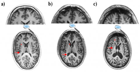
The increasing popularity of research on automatic classification of AD progression from MRI images using machine learning methods underlines the significant role of these methods in developing computer-based decision support systems [15]. Structural deformations in the brain of an AD patient, most often observed in the medial temporal lobes and hippocampus, can be perceived with the naked eye from an MRI scan [16, 17]. Figure 1 illustrates the MRI images of subjects with CN, MCI, and AD, showing the reduction in hippocampus tissue size and increase in ventricle size as the disease progresses.
This study aims to develop an efficient early diagnosis system for patients in the MCI stage before progressing to AD. Limited studies in the literature focus on Alzheimer's diagnosis based on deep learning (DL)-based feature extraction and analysis of morphometric methods, particularly tensor-based morphometry (TBM), a medical imaging method that allows analysis of morphological brain changes [18]. However, the visual interpretation of these images can be challenging, highlighting the need for DL-based methods for automatic extraction of disease-specific features.
This research aims to enhance AD detection by integrating DL and TBM methods by comparing model performances trained with medial slices (in the x, y, and z direction) or axial slices covering the hippocampus and temporal lobe. The effect of using small kernel sizes for detailed feature extraction from local volume changes in the brain on model success was examined. While binary classification (CN, AD) studies are prevalent in the literature, multiple classification (AD, MCI, CN) studies are limited. Therefore, a multiple classification approach was adopted in this research.
The structure of this paper includes "Related Work" in chapter 2, "Methods" in chapter 3, "Result and Discussion" in chapter 4, and "Conclusion" in chapter 5.
Figure 1. MRI scans of a) CN, b) MCI, and c) AD [17]
A number of studies have been carried out to identify individuals at different stages of Alzheimer’s Disease using various algorithms and medical images [19-21]. Göker [19] analyzed the brain EEG images of Alzheimer's patients using the bidirectional long-short-term memory algorithm and obtained an accuracy rate of 98.85%. Sato et al. [20] developed a new approach based on VBM analysis to identify individuals in the early stages of the disease using quantitative susceptibility mapping (QSM). Gao and Lima [21] has shown in their studies that DL-based models are effective in distinguishing Alzheimer's patients from other cognitive disorders thanks to their ability to automatically extract features from medical images. Based on these studies, it has been seen that individuals at different stages of AD can be accurately detected using different algorithms and medical images. Early studies on AD detection through machine learning focused only on AD-related brain regions and compared classification performance and biomarkers to shed light on parameters associated with normal and pathological aging [22]. In some studies, changes in the brain other than in the region(s) examined were not considered [23]. Different studies used voxel-based measurements based on image preprocessing and feature extraction with classifier types such as SVM [24] and random forests [25], which are called traditional machine learning methods. The most popular traditional algorithm is supporting vector machines (SVM), and SVM-based studies remain the most widely used method for early diagnosis and classification of AD in the literatures [26, 27]. Traditional machine learning models developed with limited independent variables in theory may be insufficient when applied to real-world problems. That is why traditional machine learning-based methods did not achieve satisfactory performance and success, especially in large and complex data sets. The biggest reason is that real-world problems have a much more complex and unpredictable structure [28-30].
DL models can be used more effectively and successfully compared to other machine learning methods in the analysis of neuroimaging data [31]. With the introduction of higher-resolution MRI data, we can provide a higher success rate for DL models, a better performance increase in automatic screening and diagnosis of brain disorders, and even more detailed extraction of the morphometric features [32]. Convolutional neural networks (CNN), the most widely used architecture of DL currently for image classification problems, are of great interest. CNN is a neural network consisting of several layers, which is used in the field of image processing [33]. There are intensive studies on CNN based medical image processing [34, 35]. Compared to other DL techniques, CNN is preferred for disease diagnosis through neuroimaging, as it specializes in learning images. For example, Gunawardena et al. diagnosed AD in the MCI stage with an accuracy rate of 84.4% with an SVM-based model and 96% with a DL-based technique by converting the 3D sMRI images in the ADNI dataset to 2D matrices and then passing them through a series of processing. In sMRI data, the CNN-based method could detect AD with much higher success than the SVM-based method [26]. Seetha and Raja [36] achieved a high success rate of 97.5% by using small kernels due to the spatial and structural variability of the brain tumor environment in their brain tumor classification models based on CNN from MRI images. The authors reduced the core size they used in their model to 2×2 to achieve low-level features in medical images, resulting in 85.5% classification performance [36].
3.1 Data
The use of a freely available common dataset among researchers increases the credibility of the studies. For this reason, the ADNI database was used as part of this research. The ADNI is a global project dedicated to discovering, analyzing, and curing disease with the aim of slowing and stopping the progression of AD. The ADNI provides a range of datasets, offering a valuable resource for researchers aiming to detect AD in its early stages. By supplying these standardized datasets, ADNI facilitates consistent research practices and promotes the global sharing of compatible data among researchers.
The ADNI was launched in 2003 as a public-private partnership, led by Principal Investigator Michael W. Weiner, MD. The primary goal of ADNI has been to test whether serial MRI, positron emission tomography (PET), other biological markers, and clinical and neuropsychological assessment can be combined to measure the progression of MCI and early AD. As such, the investigators within the ADNI contributed to the design and implementation of ADNI and/or provided data but did not participate in analysis or writing of this report. A complete listing of ADNI investigators can be found online. (GE Healthcare, Philips Medical Systems, or Siemens) [37].
3.2 Tensor-based morphometry
For large, multi-site neuroimaging analyses and clinical trials of AD and MCI, TBM is an objective, dependable, high-throughput imaging measure [38]. TBM aims to determine local volume differences among groups of brains using deformation fields that map points in a template (x1; x2; x3) to corresponding locations in individual source pictures (y1; y2; y3) using a Jacobian matrix. The local volume differences contain information about the local stress, shear, and rotation involved in the deformation. Eq. (1) shows how to compute a Jacobian matrix [39].
$\mathbf{J}=\left[\begin{array}{lll}\partial y_1 / \partial x_1 & \partial y_1 / \partial x_2 & \partial y_1 / \partial x_3 \\ \partial y_2 / \partial x_1 & \partial y_2 / \partial x_2 & \partial y_2 / \partial x_3 \\ \partial y_3 / \partial x_1 & \partial y_3 / \partial x_2 & \partial y_3 / \partial x_3\end{array}\right]$ (1)
T1 MRI images were pre-processed by Hua et al. [40] and prepared for TBM analysis. In brief, all images were resampled to 1mm voxel sizes in x, y, and z dimensions, then non-linearly aligned to a group-average template created with 40 randomly selected control subjects, and individual Jacobian maps were estimated from the warp-fields. Deformation fields calculated for deformation-based morphometry and TBM are shown in Figure 2 [39].
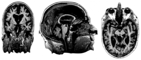
The DBM field calculates the large-scale difference between the subject image and template image, whereas the TBM field calculates local differences. TBM is a mapping method applied to MRI images to visualize brain tissue loss and enlargement. Figure 3 shows MRI image of an AD subject in the ADNI database.
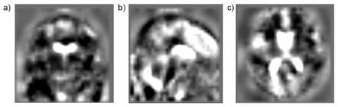
In Figure 4, the TBM analysis image of the AD subject, whose MRI image is shown in Figure 3, is presented. As can be seen in Figure 4, compared to minimally processed MRI images, TBM images are blurry and difficult to interpret by eye. This is due to the fact that TBM images present the local morphological differences of each subject compared to the group mean. They are meant to be used for group-level statistical analysis rather than visual inspection [41].
In this study, we used different variations of ADNI dataset for three different models. In the first model, the network was trained with only medial slices of three axes (axial, sagittal, and coronal) meaning that there were 3 MRI images for each subject. Then, the performance values of the network trained with those images were analyzed. 156 AD subjects [mean age: 75.4±7.5 year, 81 males (M) and 75 females (F)]; 330 patients with MCI [mean age: 74.8±7.4 year, 172 (M) and 158 (F)]; and 190 CN subjects [mean age: 76.0±5.0 years, 100 (M)/90 (F)] are used. The demographic characteristics of a total of 676 subjects used in the first model are presented in Table 1.
Figure 2. Differences between a) DBM and b) TBM [39]
Figure 3. Original MRI scan image of a single subject: a) Coronal MRI slice, b) Sagittal MRI slice and c) Axial MRI slice
Figure 4. TBM image of the subject: a) Coronal slice; b) Sagittal slice; c) Axial slice
The second and third models were trained with the same database using only slices of axial planes that cover the temporal lobes and hippocampi. Then, the performance values of these networks were analyzed. 28 AD subjects [mean age: 75.0±5.0 year, 16 males (M)/12 females (F)]; 88 patients with MCI [mean age: 73.8±5.4 years, 47 (M)/41 (F)]; and 54 CN subjects [mean age: 74.4±5.5 years, 30 (M)/24 (F)] are used. The demographic characteristics of a total of 170 subjects used in the second and third model are presented in Table 2.
Table 1. The demographic characteristics of the first model
|
Groups |
CN |
MCI |
AD |
|
Number |
190 |
330 |
156 |
|
Gender (M/F) |
100/90 |
172/158 |
81/75 |
|
Age (mean±std) |
76.0±5.0 year |
74.8±7.4 year |
75.4±7.5 year |
Table 2. The demographic characteristics of the second and third models
|
Groups |
CN |
MCI |
AD |
|
Number |
54 |
88 |
28 |
|
Gender (M/F) |
30/24 |
47/41 |
16/12 |
|
Age (mean±std) |
74.4±5.5 year |
73.8±5.4 years |
75.0±5.0 year |
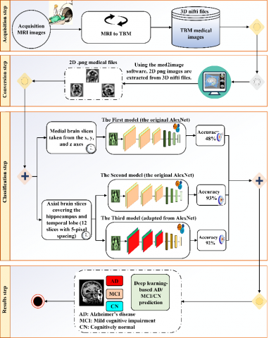
Figure 5. Obtaining the dataset used in feeding the models
3.3 Deep learning
The images, after being downloaded to our local servers, were converted to 2D png images from 3D nifti files by using med2image software [42]. 3D TBM images are downloaded from ADNI. First, the height and width of each nifti file are saved. Witht this, axial images (z axis) were sliced at 5-pixel intervals starting from the 48th pixel to the 115th pixel, covering only the hippocampus and temporal lobe. As a result, 12 2D axial png brain slices were obtained for each subject. Considering that the hippocampus and temporal lobe are the regions most affected by AD, slices with these regions in the range of 48-115 pixels were taken [6]. The steps for converting TBM images from 3D medical image format to 2D png format are presented in Figure 5.
Within the scope of this investigation, we adapted a 2D CNN-based DL architecture to diagnose AD early using TBM images. We used the AlexNet architecture, which is proven to be successful in image classification processes [43, 44]. AlexNet has won the 2012 “Imagenet Large-Scale Visual Recognition Competition” with an extraordinary difference [45]. This architecture is a deep CNN consisting of eight layers, five of which are convolutional layers with rectified linear unit (ReLU) functions and three of which are batch normalization layers. Three of the batch normalization layers are followed by max pooling layers, A learnable filter that extracts features from an input image is represented by the convolutional layer. For a 3D image of dimensions H, W, and C, where H stands for height, W for width, and C for channel count. When a three-dimensional filter is used, it can be represented as FC (number of filter channels), FH (filter height), and FW (filter width). Since AH stands for activation height and AW for activation width, the output activation map size must be AHxAW. Using the Eq. (2) and Eq. (3), activation height and width values can be calculated [46].
$A_H=1+\frac{H-F_H+2 P}{S}$ (2)
$A_W=1+\frac{W-F_W+2 P}{S}$ (3)
P stands for padding, S for stride, and since there are n filters, the dimensions of the activation map should be AWx AWxn.
The pooling layer's key purpose is to reduce the size of the feature maps. Thereby, there will be fewer parameters to learn and fewer computations to be made by the network. By applying a non-linear conversion to the given inputs, an activation function addresses non-linearity in the network [47] Eq. (4).
$\sigma(\vec{z})_i=\frac{e^{z_i}}{\sum_{j=1}^K \, e^{z_j}}$ (4)
where, $\vec{z}$ is the softmax function's input vector, and each zi value is an input vector component, which can have any real value. The normalizing term, which appears in the formula below, makes sure that the function's output values add up to 1, producing a legitimate probability distribution. K is the number of classes in the classifier with multiple classes. If the input is positive, the rectified linear activation function, or ReLU for short, will output the input directly; if it is negative, it will output zero Eq. (5). Because a model that utilizes ReLU is simpler to train and frequently performs better, it has evolved into the default activation function for many diverse types of neural networks [48].
$f_{\mathrm{ReIU}}=\max (0, x)$ (5)
In this study, we used three models. The first model that was trained using medial brain slices (in x, y, and z directions) belongs to 676 subjects (train: 1622; test: 406). In the second and third models, twelve axial brain slices obtained at 5-pixel intervals covering the hippocampus and temporal lobe from 170 subjects were used (train: 1632; test: 406). Since the number of medical images used for the training of all three models was intended to be close to each other, fewer subjects were used in the second and third models. 20% of the resulting dataset was separated as test datasets for each clinical group (AD, CN, MCI). 80% of the data was allocated for training and 20% for testing. For the training of the models, 80% of the data was used for training and 20% for testing. During model training, 20% of the training data was selected as validation data.
In our study, models are trained using AlexNet or fine-tuned AlexNet architecture. The architecture ends with two dense layers and a dropout layer with 0.5 rates between them.
In the first model, we observed the performance of original AlexNet by feeding it medial slices (in the x, y, and z directions) of TBM images from each subject. The model produced an accuracy of less than 50%, failing to perform a successful diagnosis.
For the second and third model of the study, 5-pixel-spaced axial images covering only the hippocampus and temporal lobe were extracted, yielding twelve images per subject. Hippocampus and temporal lobe were selected as the regions of interest because they are the regions that suffer the most from AD [6]. The second model that fed these images achieved over 93% accuracy using the original AlexNet network [44].
In the third model, we fine-tuned the parameters of the second model to see if we could improve the performance of the diagnosis. In the third model, in addition to implementing the original AlexNet model, an adaptation of it with a smaller kernel size and stride length was used. The idea was to make the model more consistent with the nature of the TBM images. Since they show differences in more minor scales, the kernel size and stride length were fine-tuned to catch those differences. Specifically, kernel size and stride length in the first convolutional layer were set to 3×3 and 2×2, respectively. And the strides in the first max pooling layer were changed to 2×2, the second convolutional layer was changed to 3×3 and 2×2, the second max pooling layer was changed to 2×2, the third convolutional layer was set to 2×2 and 1×1, the fourth was changed to 1×1 and 1×1, and the last max pooling layer was formed at 1×1. Naturally, the decrease in resolution caused an increase in the total learning parameters. The details of the second model can be seen in Table 3.
The accuracy of our third fine-tuned model, trained using axial slices covering the temporal lobe, was over 92%.
Table 3. Details of the CNN architecture used for the third model
|
Layer |
Output Shape |
Parameter |
|
conv2d |
113×113×96 |
2688 |
|
batch_normalization |
113×113×96 |
384 |
|
max_pooling2d |
56×56×96 |
0 |
|
conv2d_1 |
28×28×256 |
221440 |
|
batch_normalization_1 |
28×28×256 |
1024 |
|
max_pooling2d_1 |
14×14×256 |
0 |
|
conv2d_2 |
7×7×384 |
393600 |
|
batch_normalization_2 |
7×7×384 |
1536 |
|
conv2d_3 |
7×7×384 |
147840 |
|
batch_normalization_3 |
7×7×384 |
1536 |
|
conv2d_4 |
13×13×256 |
98560 |
|
batch_normalization_4 |
7×7×256 |
1024 |
|
max_pooling2d_2 |
7×7×256 |
0 |
|
flatten |
12544 |
0 |
|
dense |
4096 |
51384320 |
|
dropout |
4096 |
0 |
|
dense_1 |
10 |
40970 |
|
Total Parameter |
|
52.294.922 |
4.1 Training and evaluation of CNN models
The original size of the 2D slices is 220×200. The required image input size for AlexNet is 227 by 227. Therefore, the slices are converted to 227×227 pixels. The following parameter values were selected for all CNN models: The learning rate was chosen as 1e-5 for the models that automatically improved with adaptive moment estimation (Adam optimizer). Each model is trained for 50 epochs. The reason for this is that the validation loss value was chosen as the early stop in the second model with the best performance. In 47 steps, the model reached its automatic optimum value. For this reason, the number of steps was chosen at 50 to train all three models under equal conditions. Since there are more than two output labels, “categorical crossentropy” and “categorical accuracy” functions are used for loss and accuracy in classification models, respectively. For the training of the models, two different data sets were trained on three different models. The data sets that feed the models are not balanced. Therefore, after calculating the accuracy of all three models, the model with the best accuracy was determined. The precision, recall, and F-Score values of this model have been calculated. The study was carried out in the Google Colab environment. The flow chart of the Alzheimer's diagnosis proposed in the present study is shown in Figure 6.
Figure 6. The Alzheimer's diagnosis flowchart proposed in the present study [0: AD; 1: CN; 2: MCI]
A classification problem's performance is calculated using a confusion matrix. It is a table containing four different combinations of predicted and actual values: True positive (TP), true negative (TN), false positive (FP), and false negative (FN). Hence, accuracy (ACC-Eq. (6)), F-Score (F-SCR-Eq. (7)), precision (PRE-Eq. (8)), recall (Eq. (9)), and specificity (SP-Eq. (10)) are defined as [49]:
$A C C=\frac{T P+T N}{T P+T N+F P+F N}$ (6)
$F-S C R=\frac{2 * P R E * Recall}{P R E+Recall }$ (7)
$P R E=\frac{T P}{T P+F P}$ (8)
$Recall=\frac{T P}{T P+F N}$ (9)
$S P=\frac{T N}{T N+F P}$ (10)
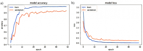
In the first model that was trained with the medial slices, accuracy was below 0.5. However, performance was greatly improved in the second and third methods, where axial slices covering the hippocampus and temporal lobe were used to feed the models (Figure 7, Figure 8.). In the second model, the training accuracy was 93%, and the loss was 0.22. The pattern of the graphs does not show any sign of overfitting. When evaluated on the test set, the model was still successful with 89% accuracy. The results show that local morphological atrophy patterns around hippocampal and temporal regions can successfully predict AD and MCI. The accuracy of a subsequent model, in which the CNN algorithm was forced to learn finer details of the images, was comparable to the previous one (92%) (Table 4).
Table 4. Accuracy and loss parameters of the models used in this study
|
Model |
Accuracy |
Loss |
|
Medial slices |
0.47 |
0.86 |
|
Temporal lobe |
0.93 |
0.22 |
|
Temporal lobe with smaller kernel |
0.92 |
0.19 |
Some models were trained with raw MRI and processed morphometric datasets, respectively, using different traditional methods. Morphometric methods were found to be able to achieve higher accuracy compared to raw MRI data [50]. Although the TBM images contained information about minor regional differences, extracting more details from the images did not alter their accuracy as expected. Chen et al. used a VBM analysis-based approach on 3D images with AlexNet, VGGNET, GoogleNet, and ResNet. The most successful results were obtained from the AlexNet and GoogleNet architectures [51]. Therefore, the high success of the AlexNet architecture used in this study supports the previous finding, showing that it can be used in morphology-based classification processes. Although using AlexNet achieved an accuracy rate of 96.22%, which is approximately four points better than the one in the current study (93%), the results show that TBM-based analyses can succeed as highly as VBM analyses. In their CNN-based method used in study [36] to diagnose brain tumors from small local deformations, they improved the accuracy of the model by reducing the core size of the mesh.
Figure 7. Loss and accuracy of the training and validation sets for the original AlexNet model trained with the axial slices (The second model)
Figure 8. Loss and accuracy of the training and validation data for the fine-tuned AlexNet model trained with the axial slices (The third model)
4.2 Comparative of results with literature
Classifier performance can be measured with a confusion matrix based on a set of predictive data whose true values are known beforehand. Typically, in the matrix, instances of a predicted class are represented in each column, while instances of a real class are represented in each row. The diagonal of the matrix shows how many samples belonging to the same class are classified correctly, and the remaining squares show how many samples belonging to the two classes are incorrectly classified. Accordingly, the confusion matrix of our second model, which has the highest accuracy among the proposed models, is presented in Figure 9, where [0: AD; 1: CN; 2: MCI] shows the actual diagnostic results of the samples in each row and the predictive diagnostic results of the samples in each column (Table 5).
Table 5. Compared with other studies in the literature
|
Reference |
Biomarker |
Database |
Method(s) |
ACC (AD, MCI, CN) |
Dataset |
Approach |
|
8 |
FDG-PET |
ADNI |
RF+RFSVM |
CN/MCI: 90.53% |
272 |
ROI based |
|
20 |
VBM |
Hokkaido University Hospital |
SVM |
CN/AD: 94% |
111 |
ROI |
|
CN/MCI: 87% |
||||||
|
MCI/AD: 68% |
||||||
|
26 |
sMRI |
ADNI |
SVM |
84.4% |
504 |
2D subject level |
|
CNN |
96% |
|||||
|
51 |
VBM |
ADNI |
LeNet |
93.83% |
479 |
3D subject level |
|
AlexNet |
96.22% |
|||||
|
VGGNet |
96.08% |
|||||
|
GoogLeNet |
97.15% |
|||||
|
ResNet |
94.60% |
|||||
|
53 |
MRI |
ADNI |
EfficientNetB3 |
97.28% |
2182 |
- |
|
54 |
fMRI |
ADNI |
VGG19 |
90% |
54 |
2D subject level |
|
Inception v3 |
85% |
|||||
|
ResNet50 |
70% |
|||||
|
55 |
MRI |
ADNI |
CNN+SVM |
97.77% |
465 |
3D subject level |
|
56 |
MRI |
ADNI |
SNN+CNN |
CN/AD: 90.15% |
450 |
ROI |
|
MCI/AD: 87.30% |
||||||
|
CN/MCI: 83.90% |
||||||
|
CNN |
CN/AD: 86.90% |
|||||
|
MCI/AD: 83.25% |
||||||
|
CN/MCI: 76.70% |
||||||
|
57 |
VBM |
ADNI |
CNN |
CN/MCI: 80.9% |
184 |
ROI |
|
59 |
VBM |
ADNI |
SegNet+ResNet-101 |
95% |
240 |
ROI |
|
60 |
DBM |
ADNI |
SVM |
CN/AD: 96.5% |
427 |
ROI |
|
CN/MCI: 91.74% |
Figure 9. Confusion matrix of the second model
Table 6 presents the precision, sensitivity, and F1-score values obtained for the test data of second model.
Table 6. Precision, sensitivity and F1-score values of the second model obtained from test data
|
|
Precision |
Sensitivity |
F1-Score |
|
0:AD |
0.91 |
0.74 |
0.82 |
|
1:CN |
0.95 |
0.82 |
0.88 |
|
2: MCI |
0.85 |
0.88 |
0.92 |
|
Average accuracy |
|
0.89 |
|
When these values are analyzed, it is seen that the highest precision score is obtained in the estimation of CN. This demonstrates that the model can perform CN prediction (95%) with higher precision compared to MCI and AD. When the sensitivity values are analyzed, the MCI (88%) and AD value (74%) are calculated, respectively. This indicates that the model was able to weed out non-MCI subjects at a high rate compared to AD subjects. Our data set is not evenly distributed. For this reason, F1 scores should be evaluated. It is seen that MCI's estimations (92% accuracy) have the highest accuracy. This implies that most datasets belong to the MCI class, and the model learns this well. In addition, the average accuracy value of the test data was calculated at 0.89, which shows that the model achieved high success not only in the training and validation data but also in the testing data.
In their study, a number of deep learning-based methods, including AlexNet, achieved higher accuracy compared to traditional machine learning methods [52]. Similar to previous studies, the AD diagnosis was made with high accuracy using AlexNet in this study (93%). Achieved 97.28% accuracy in the training dataset with the EfficientNetB3 pre-trained network [53]. However, the AlexNet network was able to achieve an accuracy of 89.95% on the test data. In another transfer learning method, they used three different DNN models (VGG19, Inception v3, and ResNet50) to predict MCI stage. They used an fMRI dataset to predict multiclass AD stages. And achieved the highest accuracy of 90% with the VGG19 network [54]. The studies of Huang et al. [53] and Zheng et al. [54] were able to achieve this accuracy with the help of the weights obtained from the pre-trained networks, while we acquired 89% accuracy by training our model on a limited dataset. In their study on the early diagnosis of AD as a multi-classification problem, they found a high accuracy rate of 97.77% [55]. However, this high accuracy was achieved by adopting an approach based on the CNN and SVM methods using a 3D dataset. This method is costly, and in our study, we adopted a more cost-effective approach by using 2D slices obtained from the affected areas. The spiking deep convolutional neural network-based pipeline designed by Savaş [56] achieved 83.90% accuracy in CN/MCI classification. they analyzed cerebral grey matter changes in MCI using VBM and acquired 80.9% accuracy for CN/MCI prediction [57]. The method proposed in this study is superior to studies [56, 57] methods; it offers a solution to the triple classification problem with 89% accuracy.
TBM-based methods used in hippocampus tissue analysis are more accurate than volumetric measurements for the diagnosis of AD and MCI [58]. This implies parallel results with this study, in which TBM-based hippocampus analysis was performed with DL methods. High accuracy was achieved with DL-based TBM analysis, which is compatible with the literature. Despite the relatively unstable nature of the dataset, as compared to the findings reported in the literature, the study [59] achieved notable accuracy levels (95%) in their respective studies by employing DL-based VBM morphometric analysis. However, they achieved this accuracy with the help of transfer learning. This signifies that DL-based morphometric analysis can be used in AD diagnosis. Raju et al. [60] found the CN/AD classification with 96.5% high accuracy, whereas the CN/MCI classification was diagnosed with 91.74% accuracy. In the proposed study, an accuracy rate of 93% was obtained. This can be attributed to DBM analyzes the disturbances at the macro level. Volumetric changes in the brain are greater in CN/AD classification problems. Volumetric changes in the brain are greater in CN/AD classification problems. Nevertheless, in the case of CN/MCI or MCI/AD classification problems, the diagnostic accuracy for micro-level deformations tested using the DBM-based method has been hindered due to the relatively limited volumetric changes. TBM analyzes local shape differences at a microlevel. TBM-based morphometric analysis can be recommended as a more successful method for early diagnosis of the disease, especially in the MCI stage. VBM, DBM, and TBM analysis-based morphometric methods have been used for AD diagnosis. When these methods were examined, their overall accuracy was over 85%. These are presented in Table 5.
In the study conducted with traditional machine learning-based methods, accuracy (MCI/AD: 68%) was low compared to DL-based methods [20]. In this research based on deep learning, higher accuracy was obtained than with traditional methods. We obtained an accuracy of 93%. This is because DBM analyzes disturbances at the macrolevel. TBM examines local shape differences at a finer scale. TBM-based morphometric analysis can be recommended as a more successful method for the early diagnosis of the disease, especially in the MCI stage. In conclusion, this study demonstrates the effectiveness of DL methods for predicting neurodegenerative diseases using TBM images. It has been demonstrated that morphological changes, especially in the hippocampal and temporal regions, can be used to successfully predict these diseases. Moreover, the results of the study show that DL-based morphological analysis outperforms SVM-based classification.
This study presents a new method to distinguish between AD, MCI, and CN stages using TBM and DL techniques. The study proposed three different models to differentiate between subjects. In addition, TBM-based analyses are compared with VBM-based analyses used in previous studies. Local morphological changes are helpful in identifying AD and MCI. As a result, TBM-based analyses achieve similar success levels compared to VBM-based analyses. The CNN-based methodology employed Within the confines of this study effectively discriminates between individuals with AD and those with MCI based on localized morphological alterations quantified through TBM. Consistent with its concept, TBM was useful only when the brain regions that are subject to the most severe local atrophy (namely, the hippocampi and temporal lobes) were used to feed the CNN algorithm. When medial slices from each axis were used, although they also contained meaningful information such as larger ventricles in AD subjects, the CNN algorithm was not able to capture the differences. However, this was not the case for the studies that used VBM or sMRI as input. A high level of predictive accuracy was reached for different 2D ROIs (covering the hippocampus). TBM is more suitable to diagnose diseases or abnormalities that are associated with a fairly small region in the brain, such as tumors, and the regions that are susceptible to atrophy should be chosen as the region of interest to run the prediction algorithm. The results show that TBM analysis using DL-based methods can be successfully used as an effective and usable method in the early diagnosis of Alzheimer's. Although the TBM contained information about minor regional differences, extracting more details using small kernels from the images did not significantly alter the model results. According to the results of all models in the study, DL-based systems can successfully perform early detection of Alzheimer's using TBM covering the hippocampus. In addition, TBM can be more successful than DBM-based morphometric methods in the early diagnosis of Alzheimer's.
This study brings a new perspective to research in this area. In future studies, researchers should explore other neural networks such as Xception, MobileNet, and newer state-of-the-art networks to construct the classifier. Additionally, they can experiment with preprocessing steps like skull stripping and density normalization to achieve similar or better results. Furthermore, by leveraging the feature extraction ability of pre-trained models, they can enhance the overall performance of the different classifiers they propose.
Data collection and sharing for this project was funded by the Alzheimer’s Disease Neuroimaging Initiative (ADNI) (National Institutes of Health Grant U01 AG024904) and DOD ADNI (Department of Defense award number W81XWH-12-2-0012). ADNI is funded by the National Institute on Aging, the National Institute of Biomedical Imaging and Bioengineering, and through generous contributions from the following: AbbVie, Alzheimer’s Association; Alzheimer’s Drug Discovery Foundation; Araclon Biotech; BioClinica, Inc.; Biogen; Bristol-Myers Squibb Company; CereSpir, Inc.; Cogstate; Eisai Inc.; Elan Pharmaceuticals, Inc.; Eli Lilly and Company; EuroImmun; F. Hoffmann-La Roche Ltd and its affiliated company Genentech, Inc.; Fujirebio; GE Healthcare; IXICO Ltd.; Janssen Alzheimer Immunotherapy Research & Development, LLC.; Johnson & Johnson Pharmaceutical Research & Development LLC.; Lumosity; Lundbeck; Merck & Co., Inc.; Meso Scale Diagnostics, LLC.; NeuroRx Research; Neurotrack Technologies; Novartis Pharmaceuticals Corporation; Pfizer Inc.; Piramal Imaging; Servier; Takeda Pharmaceutical Company; and Transition Therapeutics. The Canadian Institutes of Health Research is providing funds to support ADNI clinical sites in Canada. Private sector contributions are facilitated by the Foundation for the National Institutes of Health (www.fnih.org). The grantee organization is the Northern California Institute for Research and Education, and the study is coordinated by the Alzheimer’s Therapeutic Research Institute at the University of Southern California. ADNI data are disseminated by the Laboratory for Neuro Imaging at the University of Southern California.
[1] Avan, A., Hachinski, V. (2023). Global, regional, and national trends of dementia incidence and risk factors, 1990-2019: A global burden of disease study. Alzheimer's & Dementia, 19(4): 1281-1291. https://doi.org/10.1002/alz.12764
[2] World Health Organization. Dementia. https://www.who.int/news-room/fact-sheets/detail/dementia, accessed on December 01, 2022.
[3] Chowdhary, N., Barbui, C., Anstey, K.J., Kivipelto, M., Barbera, M., Peters, R., Zheng, L., Kulmala, J., Stephen, R., Ferri, C.P., Joanette, Y., Wang, H., Comas-Herrera, A., Alessi, C., Suharya (Dy), K., Mwangi, K.J., Petersen, R.C., Motala, A.A., Mendis, S., Prabhakaran, D., Sorefan, A.B.M., Dias, A., Gouider, R., Shahar, S., Ashby-Mitchell, K., Prince, M., Dua, T. (2022). Reducing the risk of cognitive decline and dementia: WHO recommendations. Frontiers in Neurology, 12: 765584. https://doi.org/10.3389/fneur.2021.765584
[4] Clifford, P.M., Zarrabi, S., Siu, G., Kinsler, K.J., Kosciuk, M.C., Venkataraman, V., D’Andrea, M.R., Dinsmore, S., Nagele, R.G. (2007). Aβ peptides can enter the brain through a defective blood-brain barrier and bind selectively to neurons. Brain Research, 1142: 223-236. https://doi.org/10.1016/j.brainres.2007.01.070
[5] Muralidar, S., Ambi, S.V., Sekaran, S., Thirumalai, D., Palaniappan, B. (2020). Role of tau protein in Alzheimer’s Disease: The prime pathological player. International Journal of Biological Macromolecules, 163: 1599-1617. https://doi.org/10.1016/j.ijbiomac.2020.07.327
[6] Lo, R.Y., Hubbard, A.E., Shaw, L.M., Trojanowski, J.Q., Petersen, R.C., Aisen, P.S., Weiner, M.W., Jagust, W.J. (2011). Longitudinal change of biomarkers in cognitive decline. Archives of Neurology, 68(10): 1257-1266. https://doi.org/10.1001/archneurol.2011.123
[7] Naz, S., Ashraf, A., Zaib, A. (2022). Transfer learning using freeze features for Alzheimer neurological disorder detection using ADNI dataset. Multimedia Systems, 28(1): 85-94. https://doi.org/10.1007/s00530-021-00797-3
[8] Lu, S., Xia, Y., Cai, W., Fulham, M., Feng, D.D. (2017). Early identification of mild cognitive impairment using incomplete random forest-robust support vector machine and FDG-PET imaging. Computerized Medical Imaging and Graphics, 60: 35-41. https://doi.org/10.1016/j.compmedimag.2017.01.001
[9] Wu, L., Rosa-Neto, P., Gauthier, S. (2011). Use of biomarkers in clinical trials of Alzheimer Disease: From concept to application. Molecular Diagnosis & Therapy, 15: 313-325. https://doi.org/10.1007/BF03256467
[10] Feldman, H.H., Ferris, S., Winblad, B., Sfikas, N., Mancione, L., He, Y., Tekin, S., Burns, A., Cummings, J., del Ser, T., Inzitari, D., Orgogozo, J.M., Sauer, H., Scheltens, P., Scarpini, E., Herrmann, N., Farlow, M., Potkin, S., Charles, H.C., Fox, N.C., Lane, R. (2007). Effect of rivastigmine on delay to diagnosis of Alzheimer’s Disease from mild cognitive impairment: The InDDEx study. The Lancet Neurology, 6(6): 501-512. https://doi.org/10.1016/S1474-4422(07)70109-6
[11] Kumar, L.K., Srinivasa Rao, P., Sreenivasa Rao, S. (2022). A Framework for early recognition of Alzheimer’s using machine learning approaches. In Intelligent System Design: Proceedings of India. Singapore: Springer Nature Singapore, pp. 1-13. https://doi.org/10.1007/978-981-19-4863-3_1
[12] Çelebi, S.B., Emiroğlu, B.G. (2023). Deep learning based morphometric analysis for Alzheimer's diagnosis. Journal of the Institute of Science and Technology, 13(3): 1454-1467. https://doi.org/10.21597/jist.1275669
[13] Fjell, A.M., McEvoy, L., Holland, D., Dale, A.M., Walhovd, K.B., Alzheimer’s Disease neuroimaging initiative. (2014). What is normal in normal aging? Effects of aging, amyloid and Alzheimer’s Disease on the cerebral cortex and the hippocampus. Progress in Neurobiology, 117: 20-40. https://doi.org/10.1016/j.pneurobio.2014.02.004
[14] Çelebi, S.B., Emiroğlu, B.G. (2023). A novel deep dense block-based model for detecting Alzheimer’s Disease. Applied Sciences, 13(15): 8686. https://doi.org/10.3390/app13158686
[15] Wang, Y., Wang, C., Wu, B., Chen, T., Xie, H., Ogihara, A., Ma, X.W., Zhou, S.Y., Huang, S.Q., Li, S.W., Liu, J.K., Li, K. (2022). A new early warning method for human-computer interaction of Alzheimer’s Disease patients based on deep learning. Traitement du Signal, 39(5): 1655-1662. https://doi.org/10.18280/ts.390523
[16] Sankar, T., Chakravarty, M.M., Bescos, A., Lara, M., Obuchi, T., Laxton, A.W., McAndrews, M.P., Tang-Wai, D.F., Workman, C.I., Smith G.S., Lozano, A.M. (2015). Deep brain stimulation influences brain structure in Alzheimer’s Disease. Brain Stimulation, 8(3): 645-654. https://doi.org/10.1016/j.brs.2014.11.020
[17] Chandra, A., Dervenoulas, G., Politis, M., Alzheimer’s Disease Neuroimaging Initiative. (2019). Magnetic resonance imaging in Alzheimer’s Disease and mild cognitive impairment. Journal of Neurology, 266: 1293-1302. https://doi.org/10.1007/s00415-018-9016-3
[18] Takao, H., Amemiya, S., Abe, O. (2021). Reproducibility of brain volume changes in longitudinal voxel-based morphometry between non-accelerated and accelerated magnetic resonance imaging. Journal of Alzheimer’s Disease, 83(1): 281-290. https://doi.org/10.3233/JAD-210596
[19] Göker, H. (2023). Welch spectral analysis and deep learning approach for diagnosing Alzheimer’s Disease from resting-state EEG recordings. Traitement du Signal, 40(1): 257-264. http://doi.org/10.18280/ts.400125
[20] Sato, R., Kudo, K., Udo, N., Matsushima, M., Yabe, I., Yamaguchi, A., Tha, K.K., Sasaki, M., Harada, M., Matsukawa, N., Amemiya, T., Kawata, Y., Bito, Y., Ochi, H., Shirai, T. (2022). A diagnostic index based on quantitative susceptibility mapping and voxel-based morphometry may improve early diagnosis of Alzheimer’s Disease. European Radiology, 32(7): 4479-4488. https://doi.org/10.1007/s00330-022-08547-3
[21] Gao, S., Lima, D. (2022). A review of the application of deep learning in the detection of Alzheimer’s Disease. International Journal of Cognitive Computing in Engineering, 3: 1-8. https://doi.org/10.1016/j.ijcce.2021.12.002
[22] Salvatore, C., Battista, P., Castiglioni, I. (2016). Frontiers for the early diagnosis of AD by means of MRI brain imaging and support vector machines. Current Alzheimer Research, 13(5): 509-533.
[23] Rathore, S., Habes, M., Iftikhar, M.A., Shacklett, A., Davatzikos, C. (2017). A review on neuroimaging-based classification studies and associated feature extraction methods for Alzheimer’s Disease and its prodromal stages. NeuroImage, 155: 530-548. https://doi.org/10.1016/j.neuroimage.2017.03.057
[24] Zhang, J., Yan, B., Huang, X., Yang, P., Huang, C. (2008). The diagnosis of Alzheimer’s Disease based on voxel-based morphometry and support vector machine. In 2008 Fourth International Conference on Natural Computation, 2: 197-201, IEEE. https://doi.org/10.1109/ICNC.2008.804.
[25] Zhang, F., Tian, S., Chen, S., Ma, Y., Li, X., Guo, X. (2019). Voxel-based morphometry: Improving the diagnosis of Alzheimer’s Disease based on an extreme learning machine method from the ADNI cohort. Neuroscience, 414: 273-279. https://doi.org/10.1016/j.neuroscience.2019.05.014
[26] Gunawardena, K.A.N.N.P., Rajapakse, R.N., Kodikara, N.D. (2017). Applying convolutional neural networks for pre-detection of Alzheimer’s Disease from structural MRI data. In 2017 24th International Conference on Mechatronics and Machine Vision in Practice (M2VIP). IEEE, pp. 1-7. https://doi.org/10.1109/M2VIP.2017.8211486
[27] Sarica, A., Cerasa, A., Quattrone, A. (2017). Random forest algorithm for the classification of neuroimaging data in Alzheimer’s Disease: A systematic review. Frontiers in Aging Neuroscience, 9: 329. https://doi.org/10.3389/fnagi.2017.00329
[28] Çalışkan, A. (2022). A new ensemble approach for congestive heart failure and arrhythmia classification using shifted one-dimensional local binary patterns with long short-term memory. The Computer Journal, 65(9): 2535-2546. https://doi.org/10.1093/comjnl/bxac087
[29] Saglam, M., Spataru, C., Karaman, O.A. (2022). Electricity demand forecasting with use of artificial intelligence: The case of gokceada island. Energies, 15(16): 5950. https://doi.org/10.3390/en15165950
[30] Polat, H. (2022). Time-frequency complexity maps for EEG-based diagnosis of Alzheimer’s Disease using a lightweight deep neural network. Traitement du Signal, 39(6): 2103-2113. https://doi.org/10.18280/ts.390623
[31] Shen, D., Wu, G., Suk, H.I. (2017). Deep learning in medical image analysis. Annual Review of Biomedical Engineering, 19: 221-248. https://doi.org/10.1146/annurev-bioeng-071516-044442
[32] Somasundaram, K., Genish, T. (2015). An atlas-based approach to segment the hippocampus from MRI of human head scans for the diagnosis of Alzheimers disease. International Journal of Computational Intelligence and Informatics, 5(1). https://doi.org/10.1016/j.zemedi.2018.11.002
[33] Mikołajczyk, A., Grochowski, M. (2018). Data augmentation for improving deep learning in image classification problem. In 2018 International Interdisciplinary PhD Workshop (IIPhDW). IEEE, pp. 117-122. https://doi.org/10.1109/IIPHDW.2018.8388338
[34] Jiang, Y. (2021). Application of deep learning and brain images in diagnosis of Alzheimer’s patients. Traitement du Signal, 38(5): 1431-1438. https://doi.org/10.18280/ts.380518
[35] Diker, A., Sönmez, Y., Özyurt, F., Avcı, E., Avcı, D. (2021). Examination of the ECG signal classification technique DEA-ELM using deep convolutional neural network features. Multimedia Tools and Applications, 80: 24777-24800. https://doi.org/10.1007/s11042-021-10517-8
[36] Seetha, J., Raja, S.S. (2018). Brain tumor classification using convolutional neural networks. Biomedical & Pharmacology Journal, 11(3): 1457. http://dx.doi.org/10.13005/bpj/1511
[37] Jack Jr, C.R., Bernstein, M.A., Fox, N.C., Thompson, P., Alexander, G., Harvey, D., RTR, B.B., Britson, P.J., Whitwell, J.L., Ward, C., Dale, A.M., Felmlee, J.P., Gunter, J.L., Hill, D.L.G., Killiany, R., Schuff, N., Fox-Bosetti, S., Lin, C., Studholme, C., DeCarli, C.S., Krueger, G., Ward, H.A., Metzger, G.J., Scott, K.T., Mallozzi, R., Blezek, D., Levy, J., Debbins, J.P., Fleisher, A.S., Albert, M., Green. R., Bartzokis, G., Glover, G., Mugler J., Weiner, M.W. (2008). The Alzheimer’s Disease neuroimaging initiative (ADNI): MRI methods. Journal of Magnetic Resonance Imaging: An Official Journal of the International Society for Magnetic Resonance in Medicine, 27(4): 685-691. https://doi.org/10.1002/jmri.21049
[38] Hua, X., Hibar, D.P., Ching, C.R., Boyle, C.P., Rajagopalan, P., Gutman, B.A., Leow, A.D., Toga, A.W., Jack, C.R., Harvey, D., Weiner, M.W., Thompson, P.M., Alzheimer’s Disease Neuroimaging Initiative. (2013). Unbiased tensor-based morphometry: Improved robustness and sample size estimates for Alzheimer’s Disease clinical trials. Neuroimage, 66: 648-661. https://doi.org/10.1016/j.neuroimage.2012.10.086
[39] Ashburner, J., Friston, K. (2003). Morphometry, human brain function. Wellcome Dept. of Imaging Neuroscience, 2nd ed., Vol. 6.
[40] Hua, X., Leow, A.D., Parikshak, N., Lee, S., Chiang, M.C., Toga, A.W., Jack, C.R., Weiner, M.W., Thompson, P.M., Alzheimer’s Disease Neuroimaging Initiative. (2008). Tensor-based morphometry as a neuroimaging biomarker for Alzheimer’s Disease: An MRI study of 676 AD, MCI, and normal subjects. Neuroimage, 43(3): 458-469. https://doi.org/10.1016/j.neuroimage.2008.07.013
[41] Paniagua, B., Ehlers, C., Crews, F., Budin, F., Larson, G., Styner, M., Oguz, I. (2011). Using tensor-based morphometry to detect structural brain abnormalities in rats with adolescent intermittent alcohol exposure. In Medical Imaging 2011: Biomedical Applications in Molecular, Structural, and Functional Imaging. SPIE, 7965: 204-210. https://doi.org/10.1117/12.878389
[42] Pienaar, R. (2023). Med2image 2.6.6. GitHub. https://github.com/FNNDSC/med2image.
[43] Wagle, S.A. (2021). Comparison of plant leaf classification using modified AlexNet and support vector machine. Traitement du Signal, 38(1): 79-87. https://doi.org/10.18280/ts.380108
[44] Krizhevsky, A., Sutskever, I., Hinton, G.E. (2012). Imagenet classification with deep convolutional neural networks. Advances in Neural Information Processing Systems, 25.
[45] Eldem, H., Ülker, E., Işıklı, O.Y. (2023). Effects of training parameters of AlexNet architecture on wound image classification. Traitement du Signal, 40(2): 811-817. https://doi.org/10.18280/ts.400243
[46] Mohi ud din dar, G., Bhagat, A., Ansarullah, S.I., Othman, M.T.B., Hamid, Y., Alkahtani, H.K., Ullah, I., Hamam, H. (2023). A novel framework for classification of different Alzheimer’s Disease stages using CNN model. Electronics, 12(2): 469. https://doi.org/10.3390/electronics12020469
[47] Sharma, S., Sharma, S., Athaiya, A. (2017). Activation functions in neural networks. International Journal of Engineering Applied Sciences and Technology, 6(12): 310-316.
[48] Nair, V., Hinton, G.E. (2010). Rectified linear units improve restricted Boltzmann machines. In Proceedings of the 27th International Conference on Machine Learning (ICML-10), pp. 807-814.
[49] Krstinić, D., Braović, M., Šerić, L., Božić-Štulić, D. (2020). Multi-label classifier performance evaluation with confusion matrix. Computer Science & Information Technology, 1. https://doi.org/10.5121/csit.2020.100801
[50] Ota, K., Oishi, N., Ito, K., Fukuyama, H., Sead-J Study Group. (2014). A comparison of three brain atlases for MCI prediction. Journal of Neuroscience Methods, 221: 139-150. https://doi.org/10.1016/j.jneumeth.2013.10.003
[51] Chen, S., Zhang, J., Wei, X., Zhang, Q. (2020). Alzheimer’s Disease classification using structural MRI based on convolutional neural networks. In Proceedings of the 2020 2nd International Conference on Big-data Service and Intelligent Computation, pp. 7-13. https://doi.org/10.1145/3440054.3440056
[52] Turkson, R.E., Qu, H., Mawuli, C.B., Eghan, M.J. (2021). Classification of Alzheimer’s Disease using deep convolutional spiking neural network. Neural Processing Letters, 53: 2649-2663. https://doi.org/10.1007/s11063-021-10514-w
[53] Huang, H., Zheng, S., Yang, Z., Wu, Y., Li, Y., Qiu, J., Cheng, Y., Lin, P., Lin, Y., Guan, J., Mikulis, D.J., Zhou, T., Wu, R. (2023). Voxel-based morphometry and a deep learning model for the diagnosis of early Alzheimer’s Disease based on cerebral gray matter changes. Cerebral Cortex, 33(3): 754-763. https://doi.org/10.1093/cercor/bhac099
[54] Zheng, W., Liu, H., Li, Z., Li, K., Wang, Y., Hu, B., Dong, Q., Wang, Z. (2023). Classification of Alzheimer’s Disease based on hippocampal multivariate morphometry statistics. CNS Neuroscience & Therapeutics. https://doi.org/10.1111/cns.14189
[55] Buvaneswari, P.R., Gayathri, R. (2021). Deep learning-based segmentation in classification of Alzheimer’s Disease. Arabian Journal for Science and Engineering, 46: 5373-5383. https://doi.org/10.1007/s13369-020-05193-z
[56] Savaş, S. (2022). Detecting the stages of Alzheimer’s Disease with pre-trained deep learning architectures. Arabian Journal for Science and Engineering, 47(2): 2201-2218. https://doi.org/10.1007/s13369-021-06131-3
[57] Thayumanasamy, I., Ramamurthy, K. (2022). Performance analysis of machine learning and deep learning models for classification of Alzheimer’s Disease from brain MRI. Traitement du Signal, 39(6): 1961-1970. https://doi.org/10.18280/ts.390608
[58] Long, X., Chen, L., Jiang, C., Zhang, L., Alzheimer’s Disease Neuroimaging Initiative. (2017). Prediction and classification of Alzheimer disease based on quantification of MRI deformation. PloS One, 12(3): e0173372. https://doi.org/10.1371/journal.pone.0173372
[59] Abed, M.T., Fatema, U., Nabil, S.A., Alam, M.A., Reza, M.T. (2020). Alzheimer’s Disease prediction using convolutional neural network models leveraging pre-existing architecture and transfer learning. In 2020 Joint 9th International Conference on Informatics, Electronics & Vision (ICIEV) and 2020 4th International Conference on Imaging, Vision & Pattern Recognition (icIVPR). IEEE, pp. 1-6. https://doi.org/10.1109/ICIEVicIVPR48672.2020.9306649
[60] Raju, M., Gopi, V.P., Anitha, V.S., Wahid, K.A. (2020). Multi-class diagnosis of Alzheimer’s Disease using cascaded three dimensional-convolutional neural network. Physical and Engineering Sciences in Medicine, 43: 1219-1228. https://doi.org/10.1007/s13246-020-00924-w