Youssef Toulni*![]() | Benayad Nsiri
| Benayad Nsiri![]() | Taoufiq Belhoussine Drissi
| Taoufiq Belhoussine Drissi![]()
© 2023 IIETA. This article is published by IIETA and is licensed under the CC BY 4.0 license (http://creativecommons.org/licenses/by/4.0/).
OPEN ACCESS
The diagnosis techniques of diseases which are based on biomedical signals processing are constantly evolving, cardiovascular diseases are no exception to the other biomedical signals. Thanks to the development of signal processing techniques, it has been possible to extract several kinds of information from the ECG signals who told us about the heart's health. The goal of this study is to attempt to create a model based on two methods of signal processing: wavelet analysis and the determination of Mel frequency cepstral coefficients. With the help of this model, it is possible to extract statistical features and MFCC coefficients from approximation coefficients obtained when the discrete wavelet transform (DWT) is applied to analyze an ECG signal. As a result, the various features derived for each approximation coefficient will be classified using a support vector machine classifier (SVM classifier). The classifier's performance has been measured after the use a k fold cross validation technique to avoid the overfitting and the underfitting problems and making the results more reliable and credible.
electrocardiogram, discrete wavelet transform, mel frequency cepstrum coefficient, support vector machine, k- fold, cross validation
Biomedical signals are considered to be a huge amount of information deduced from the physiological activities of the human body that may be useful in diagnosing many diseases; the processing and correct interpretation of these signals provides a better understanding of the state of health of patients examined.
The electrocardiogram (ECG) is a biomedical signal that is often employed in the healthcare field because it reflects the heart's electrical activity and its use allows the diagnosis of a large variety of cardiovascular problems (cardiovascular diseases); cardiovascular disease is the world's biggest major cause of death, according to World Health Organization estimates, nearly 9 million deaths were recorded in 2019 [1], representing more than 16% of all deaths in the world.
Several heart issues can be diagnosed by analyzing ECG signals in various ways; for example, reading the electrocardiogram by a specialized person allows one to interpret and identify the state of health of the heart; however, this is not always the case. Indeed, in some cases, it is difficult to find trained people to evaluate these signals, that why we need methods more independent to any human intervention or even techniques which can do an automatic signal analysis. Thus, the field of signal processing makes a significant and effective contribution to the detection of any problem or abnormality.
As a result, various studies have been done on this subject to improve efficiency of the automated diagnosis of the ECG signal by trying to extract more information as possible from the ECG signals; these works discuss several approaches to solving issues confronted in the processing of ECG signals; for example, Dwivedi et al. [2], and Sraitih and Jabrane [3] represent various decomposition techniques of the ECG signal such as EMD, DWT, and SWT in order to denoise the signal, some research also attempts to solve this problem by employing filters, as in the case of Das and Chakraborty [4], which use FIR and IIR filters, other research such as that of Khiter et al. [5] and Chen et al. [6] choose to use adaptive filters. On the other hand, the extraction of the features which can identify the signal is based on different approaches, among these approaches We find those that depend on the signal's morphology, for instance, the identification of the QRS complex established by Pan and Tompkins [7], the determination of the RR interval or detection of peaks [8], without missing the other types of features. Also, statistical features in particular are highly helpful for signal identification [9]. Other approaches suggest the identification using a combination of several types of features such as for example the combination between the statistical and morphological features proposed in the works of Sahoo et al. [10] or in the article of Chashmi and Amirani [11] which is based on the wavelet coefficients in the feature extraction; As a consequence, we can see that the diversity of approaches and features implemented in signal diagnostics makes the selection phase crucial and demands a lot of attention.
In this paper, we will focus on Mel Frequency Cepstral Coefficients (MFCC), which are a kind of feature that have shown to be extremely successful in the field of audio signal processing [12], these coefficients will be calculated after a wavelet decomposition of the ECG signal. In addition to knowing the use of the MFCC coefficients, we will study the effect of the combination of these coefficients with the statistical features on the quality of separation between normal and pathological ECG signals, as well as the identification of the signal class will be performed using classification techniques for machine learning, which is the Support Vector Machine SVM.
This section will explain the approach used in this paper, which attempts to design a model able to process and recognize a given ECG signal using the Mel frequency cepstral coefficients obtained from the wavelet coefficients signal. First, the ECG signals from the database are pre-processed; in this step, we remove noise from the signals and calculate the wavelet coefficients; after that, for every signal, each approximation coefficient obtained just after wavelet decomposition at different scales is used to calculate two types of parameters: statistical features and Mel frequency cepstral coefficients MFCC. This leads to the establishment of a database with two distinct types of features, namely statistical features and MFCC coefficients, which will finally be fed in an SVM classifier; Figure 1 illustrates the approach used in this paper.
Figure 1. Diagram of the proposed approach
2.1 The database
The ECG signals used in this study were obtained from the MIT BIH Arrythmiya Database [13, 14], which contains 48 recordings of ECG signals sampled at 360Hz, each signal enduring half an hour and representing two distinct classes. The first class indicates sick persons, and the second class represents the healthy ones. These 48 recordings were selected among 4000 recordings. 23 of these 48 signals are chosen randomly while the remaining recordings have been selected in order to represent some significant clinical cases for the reliability of the database, 47 patients served as the study's subjects (two recordings belong to the same patient), with 25 males and 22 women whose ages ranged between 23 and 89.
2.2 Wavelet analysis
A popular signal processing method for analyzing non-stationary signals is the wavelet transform; this concept was first proposed in the 1980s [15, 16]. It is based on analyzing the time and frequency of a given signal by convolving it with a function known as the mother wavelet $\psi(t)$, this wavelet must have a finite duration, so it is a window function that checks the condition [17]:
$\int_{-\infty}^{+\infty} \psi(t) d t=0$ (1)
Additionally, the mother wavelet can shift along the time axis by a translation coefficient “a” and compress or expand through a scale coefficient “b”. As a result, the mother wavelet may be defined as follows [16, 18, 19]:
$\Psi_{\mathrm{a}, \mathrm{b}}(\mathrm{t})=\frac{1}{\mathrm{a}^{1 / 2}} \psi\left(\frac{\mathrm{t}-\mathrm{b}}{\mathrm{a}}\right)$ (2)
(a)
(b)
(c)
(d)
(e)
(f)
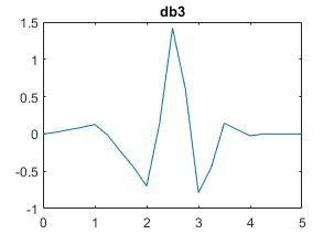
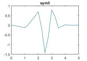
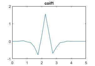
Figure 2. Some wavelet families
a is defined as the scaling coefficient and b represents the shifting one. This decomposition technique may be calculated in two ways: continuous and discrete. The first form is the CWT continuous wavelet transform, which is calculated for a given signal s (t) using the following formula [20]:
$c_{a, b}=\frac{1}{a^{1 / 2}} \int_{-\infty}^{+\infty} s(t) \psi^*\left(\frac{t-b}{a}\right) d t$ (3)
$\psi^*$ indicates the conjugate of the wavelet $\psi$. Figure 2 illustrates some of the most common mother wavelet families.
However, the continuous wavelet transform is sometimes difficult to calculate since it consumes a lot of memory and takes time during the calculation [20]. These issues are resolved by the discrete wavelet transform (DWT), characterized by its simplicity this technique decomposes the signal studied in two parts, a low frequency component and another high frequency component and that is done on several levels. This decomposition is obtained when a block of low-pass and high-pass filters are applied to the input signal in order to extract respectively the approximation and detail coefficients [15, 16, 21-23], and the coefficients of the next level are obtained by repeating the same procedure on the coefficient of approximation until the desired level is reached (see Figure 3).
Figure 3. Discrete wavelet decomposition at 2nd level of scale
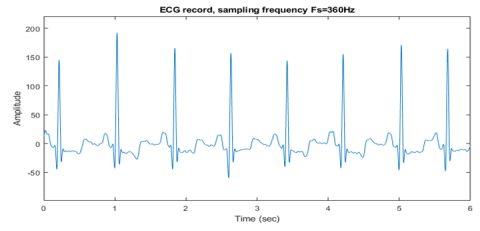
Figure 4. ECG signal from MIT-BIH Arrhythmia Database (record n° 100m)
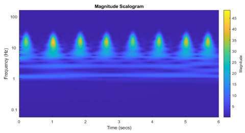
Figure 5. CWT of the ECG signal
Figure 6. Discrete wavelet transform applied to the ECG signal
The DWT is particularly effective in identifying and extracting several bits of information contained in the signal owing to its simplicity of execution and good precision in temporal and frequency resolution [22].
Figure 4 is an extract from a database recording of an ECG signal that will be analyzed using continuous and discrete wavelet transforms. The CWT localizes the information in time and frequency as shown in Figure 5, and this information is located at low frequencies (yellow areas). This is also valid for the discrete analysis (Figure 6), as we can see from the higher amplitudes of the coefficients that describe low frequencies.
2.3 Mel frequency cepstral coefficients (MFCC)
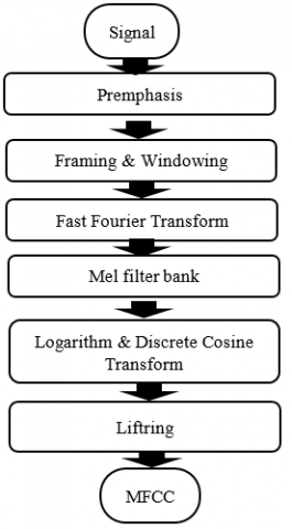
This approach is well-known for its robustness and is widely used as a technique of processing and extracting features from audio signals; it is based on the determination of cepstral coefficients; Figure 7 illustrates the process that helps us in calculating the MFCC coefficients.
Figure 7. MFCC Diagram bloc
The MFCC coefficients are extracted according to the following steps:
2.3.1 Pre-emphasis
In the pre-emphasis phase, a finite impulse response filter is used to process the signal [23], the filter used at the following transfer function [24]:
$H=1-\alpha z^{-1}$ (4)
So, the sample of the signal after pre-emphasis $s_n^{\prime}$ is:
$s_n^{\prime}=1-\alpha s_{n-1}$ (5)
This step is used to accentuate the signal's high frequency components. We choose 0.95 as the value of $\alpha$ in this study.
2.3.2 Framing and windowing
The fact that the signal is not stationary, it is necessary to divide the signal into small segments in order to be able to apply the usual signal processing techniques [23], these segments have a limited duration ranging between 40ms and 60ms. This process can lead to discontinuity between the frames of the segmented signal; thus, an overlap of about 10ms, as well as windowing of each frame of the signal, is proposed to resolve this problem [25], windowing aims to reduce signal discontinuities and make the boundaries of each frame sufficiently smooth to connect with the beginnings [26], this step is performed by multiplying the samples of the signal by the Hamming window as the following formula shows [27]:
$s_n^{\prime \prime}=w(n) s_n^{\prime}$ (6)
With w(n) the Hamming window which has the expression:
$w(n)=0.54-0.46 \cos \left(\frac{2 \pi n}{N-1}\right)$ (7)
In each frame, N is the number of the signal.
2.3.3 Discrete Fourier transform
The discrete Fourier transform is employed in this stage to move from the time domain to the frequency domain in order to collect the information contained in the ECG signal's spectrum [28].
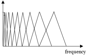
2.3.4 Mel's filter bank
The spectrum from each frame is then fed into a sequence of triangular bandpass filters that overlap with each other [25, 29], in this paper, we have chosen a bloc composed by twenty triangular filter (Figure 8); these filters are based on Mel's scale, and their characteristics are similar to those of the auditory system. The following formula is used to convert frequency f to Mel's frequency:
$m e l=2595 \log _{10}\left(1+\frac{f}{700}\right)$ (8)
Figure 8. Mel filter bank
2.3.5 Logarithm & discrete cosine transform DCT
Applying the discrete cosine transform and decimal logarithm to the energy obtained at each filter's output, the following calculation determines the MFCC coefficients by using to the following formula:
$c_i=\sqrt{\frac{2}{N}} \sum_j^N m_j \cos \left(\frac{\pi i}{N}(j-0.5)\right)$ (9)
With $m_j$ the logarithm of the energy coming from each filter's output and N the number of filters.
2.3.6 The liftering
The last step is to increase the amplitude of the higher order cepstral coefficients to make them sufficiently similar using the following relation [23, 27]:
$c_n^{\prime}=\left(1+\frac{L}{2} \sin \left(\frac{\pi n}{L}\right)\right) c_n$ (10)
2.4 Support vector machine classifier
The classification technique proposed in this study is support vector machine (SVM). SVM is a machine learning method that allows for binary classification. The goal of this method is to divide the signal's characteristics into many classes [28-30]. It is based on the development of a separation area between the various learning set classes (also called test set). The boundaries of this area are known as hyperplanes [12, 30, 31]. A good classification via this method is based on the increase of the margin located between the different hyperplanes [31, 32].
The selection of training and test sets is extremely important since it may lead to several problems that lower the model's efficiency, such as overfitting and underfitting [33]. To address these issues, we employ k fold cross validation [34, 35], which entails splitting the data set into k parts, selecting one of these parts as a test subset and the remaining k -1 parts as a training subset, and repeating this procedure k times. The accuracy of the model is determined by averaging the accuracy of each iteration.
To identify the signal, the proposed model allows to introduce an electrocardiogram (ECG) signal obtained from the MIT BIH Arrythmia database in various blocks. As we have seen we will first decompose the signal in order to remove all the noise that affects the signal, this decomposition is done using the DWT discrete wavelet transform, the coefficients extracted during the decomposition allow the detection of high frequency noise (50 Hz - 60 Hz) of various origins, such as those caused by power line interference, physical activity, or bad wiring. We discovered that these noises are mostly concentrated in the detail coefficients d1 and d2. It is also highly recommended to remove the offset generated by the baseline, which manifests in the frequency interval range [0, 0.5 Hz] and is contained in the approximation coefficient a8 [36].
We acquire a fresh denoised signal after eliminating these coefficients (d1, d2, and a8) by thresholding. The ECG signal is then decomposed for the second time in order to obtain the first eight approximation coefficients to extract the other features that include the signal's information; this step aims to extracting statistic features which are [37]:
The mean value:
$\mu=\frac{1}{N} \sum_{i=1}^N x_i$ (11)
The root mean square:
$r m s=\sqrt{\frac{1}{N} \sum_{i=1}^N x_i^2}$ (12)
The variance:
$v=\frac{1}{N} \sum_{i=1}^N\left(x_i-\mu\right)^2$ (13)
Standard deviation:
$\sigma=\sqrt{\frac{1}{N} \sum_{i=1}^N\left(x_i-\mu\right)^2}$ (14)
The skewness:
$\varphi=\frac{1}{N} \frac{\sum_{i=1}^N\left(x_i-\mu\right)^3}{\sigma^3}$ (15)
The kurtosis:
$\psi=\frac{1}{N} \frac{\sum_{i=1}^N\left(x_i-\mu\right)^4}{\sigma^4}$ (16)
Wavelet entropy:
$H=-\frac{1}{N} \sum_{i=1}^N x_i^2 \log \left(x_i^2\right)$ (17)
N signifies the number of samples, and x (t) denotes a signal that has been sampled.
Moreover, the first twelve MFCC coefficients of each of the acquired approximation coefficients are calculated, as a result, we make a data set containing seven statistical features and twelve MFCC coefficients for each record. After that comes the classification step, in this step the data set will be classified by injecting it into an SVM classifier to distinguish between two classes of patients, one class of sick patients and the other class of people concerned the healthy persons, this classifier use k fold cross validation with k = 8 to avoid overfitting the model and improve the credibility of obtained results. The following metrics are used to evaluate the performance of the classification of features acquired for each scale coefficient [38]:
$A c c=\frac{T N+T P}{T P+T N+F P+F N} \times 100$ (18)
$S e n=\frac{T P}{T P+F N} \times 100$ (19)
$S p e=\frac{T N}{T N+F P} \times 100$ (20)
TP: True positive (illustrates a normal signal that were appropriately identified)
TN: True negative (illustrates abnormal signal that were appropriately identified)
FP: False positive (reflects normal signal that were misclassified)
FN: False negative (shows abnormal signal that were misclassified)
The proposed method in this paper try to combine between two different types of features which are calculated from the wavelet coefficients which are extracted from the ECG signal, these features are the statistical features and the MFCC coefficients.
Algorithm 1. Description of the process
1: #Create empty arrays
2: {Si}i = 1, …, 8 (8 arrays for storing statistical features)
3: {Mi}i = 1, …, 8 (8 arrays for storing MFCC features)
4: LOAD ECG database, Y labels for ECG signal
5: FOR each signal from database
6: #Denoising ECG
7: Decompose the signal using DWT
8: $d_1 \leftarrow 0, d_2 \leftarrow 0, a_8 \leftarrow 0$
9: Reconstruct the signal
10: #Calculate eight first approximation coefficients
11: FOR each coefficient ai
12: Calculate statistical features
13: Calculate MFCC features
14: $S_i \leftarrow$ statistical features, $M_i \leftarrow$ MFCC features
15: end FOR
16: end FOR
17: #Classification
18: LOAD {Si}i = 1, …, 8, {Mi}i = 1, …, 8
19: FOR each i
20: Create train and test datasets [Mi Y], [Si Y]
21: and [Si Mi Y] with k fold cross validation
22: Train the models
23: Test the models
24: Store the metrics in a table
25: end FOR
26: Display the table of metrics
The exploitation of the approximation coefficients for different mother wavelets allowed us to create three different models. the first model consists of the statistical characteristics, the second is designed from the MFCC coefficients, while the last is a combination of the two previous models.
According to the results mentioned in Tables 1, 2 and 3 we note that the best accuracies are those obtained by the coefficients of approximation a7 (symlet 7 and 8) and a5 a6 for (coiflet 4 and 5), while for the second model is the coefficient a4 which gives the best accuracy.
In relation to the third model, we notice that the accuracy of the model is clearly improved in the majority of cases after the combination between the MFCC coefficients and the statistical features (see Table 1 & Table 2). Table 3 summarizes the results obtained for different wavelet families. We notice that the best result in terms of accuracy is obtained for the approximation coefficient which is extracted at the fourth scale level with the mother wavelet coiflet 4.
Table 1. Accuracy (Acc), sensitivity (Sen) and specificity (Spe) for MFCC only
|
wavelet |
Metrics |
The first eight approximation scale coefficients |
|||||||
|
a1 |
a2 |
a3 |
a4 |
a5 |
a6 |
a7 |
a8 |
||
|
Sym7 |
Acc |
35.4 |
39.6 |
66.7 |
56.3 |
64.6 |
64.6 |
77.1 |
68.1 |
|
Sen |
29.2 |
41.7 |
54.2 |
50.0 |
54.2 |
66.7 |
79.2 |
78.3 |
|
|
Spe |
41.7 |
37.5 |
79.2 |
62.5 |
75.0 |
62.5 |
75.0 |
58.3 |
|
|
Sym8 |
Acc |
47.9 |
35.4 |
50.0 |
58.3 |
64.6 |
68.8 |
77.1 |
65.2 |
|
Sen |
54.2 |
50.0 |
25.0 |
45.8 |
66.7 |
70.8 |
75.0 |
72.7 |
|
|
Spe |
41.7 |
20.8 |
75.0 |
70.8 |
62.5 |
66.7 |
79.2 |
58.3 |
|
|
Coif4 |
Acc |
46.0 |
39.8 |
52.8 |
57.1 |
63.8 |
67.8 |
67.4 |
59.7 |
|
Sen |
21.4 |
46.9 |
37.2 |
55.4 |
66.4 |
70.1 |
63.5 |
64.9 |
|
|
Spe |
70.6 |
32.6 |
68.6 |
58.8 |
61.3 |
65.4 |
71.6 |
54.4 |
|
|
Coif5 |
Acc |
46.5 |
44.8 |
68.0 |
59.7 |
73.1 |
68.2 |
68.2 |
61.7 |
|
Sen |
37.3 |
45.7 |
60.1 |
49.5 |
79.0 |
65.6 |
65.6 |
65.6 |
|
|
Spe |
55.6 |
43.1 |
75.8 |
69.9 |
67.2 |
70.8 |
70.8 |
58.1 |
|
Table 2. Accuracy, sensitivity and specificity for statistical features only
|
wavelet |
Metrics |
The first eight approximation scale coefficients |
|||||||
|
a1 |
a2 |
a3 |
a4 |
a5 |
a6 |
a7 |
a8 |
||
|
Sym7 |
Acc |
71.0 |
71.4 |
73.1 |
79.8 |
72.0 |
69.8 |
59.9 |
42.1 |
|
Sen |
76.2 |
76.6 |
77.5 |
88.9 |
85.3 |
82.6 |
61.3 |
55.7 |
|
|
Spe |
65.9 |
66.1 |
68.6 |
70.7 |
58.8 |
57.0 |
58.5 |
30.0 |
|
|
Sym8 |
Acc |
72.2 |
73.2 |
73.1 |
75.7 |
70.0 |
68.9 |
58.8 |
48.6 |
|
Sen |
76.4 |
76.7 |
78.1 |
84.6 |
79.5 |
77.7 |
66.3 |
60.1 |
|
|
Spe |
68.1 |
69.7 |
68.2 |
66.7 |
60.5 |
60.0 |
51.3 |
38.8 |
|
|
Coif4 |
Acc |
74.6 |
74.7 |
75.4 |
83.1 |
72.6 |
75.2 |
60.3 |
48.6 |
|
Sen |
81.3 |
81.6 |
82.8 |
93.8 |
81.3 |
82.8 |
72.0 |
67.5 |
|
|
Spe |
67.8 |
67.9 |
68.0 |
72.3 |
63.9 |
67.7 |
48.5 |
32.3 |
|
|
Coif5 |
Acc |
74.6 |
74.6 |
75.6 |
83.9 |
72.8 |
72.5 |
54.7 |
47.0 |
|
Sen |
81.0 |
81.2 |
82.8 |
94.6 |
81.8 |
81.4 |
63.3 |
62.7 |
|
|
Spe |
68.3 |
68.1 |
68.3 |
73.1 |
63.7 |
63.6 |
46.0 |
31.7 |
|
Table 3. Accuracy, sensitivity and specificity for MFCC and statistical features together
|
wavelet |
Metrics |
The first eight approximation scale coefficients |
|||||||
|
a1 |
a2 |
a3 |
a4 |
a5 |
a6 |
a7 |
a8 |
||
|
Sym7 |
Acc |
73.0 |
65.0 |
73.0 |
83.3 |
70.8 |
72.9 |
66.7 |
55.3 |
|
Sen |
75.0 |
67.0 |
75.0 |
95.8 |
79.2 |
79.2 |
62.5 |
60.9 |
|
|
Spe |
71.0 |
63.0 |
71.0 |
70.8 |
62.5 |
66.7 |
70.8 |
50.0 |
|
|
Sym8 |
Acc |
72.9 |
62.5 |
72.9 |
81.3 |
68.8 |
75.0 |
66.7 |
62.8 |
|
Sen |
75.0 |
66.7 |
79.7 |
95.8 |
79.7 |
79.7 |
58.3 |
63.0 |
|
|
Spe |
70.8 |
58.3 |
66.7 |
66.7 |
70.8 |
70.8 |
75.0 |
62.5 |
|
|
Coif4 |
Acc |
75.0 |
72.3 |
72.9 |
85.4 |
77.1 |
75.0 |
75.0 |
66.7 |
|
Sen |
75.0 |
79.2 |
79.7 |
95.8 |
83.3 |
83.3 |
66.7 |
66.7 |
|
|
Spe |
75.0 |
66.7 |
66.7 |
75.0 |
70.8 |
66.7 |
83.3 |
66.7 |
|
|
Coif5 |
Acc |
75.0 |
68.8 |
66.7 |
83.3 |
66.7 |
75.0 |
70.8 |
64.7 |
|
Sen |
75.0 |
75.0 |
75.0 |
95.8 |
75.0 |
79.2 |
62.5 |
66.7 |
|
|
Spe |
75.0 |
62.5 |
58.0 |
70.8 |
58.3 |
70.8 |
79.2 |
62.5 |
|
Table 4. Comparison results
|
Paper |
Used method |
Classifier |
Accuracy |
||
|
Siti [25] |
DWT d4, d5, d6 |
Haar |
KNN |
68% |
|
|
Sym 7 |
71% |
||||
|
MFCC |
85% |
||||
|
Proposed method |
DWT, a4 MFCC |
Sym7 |
SVM |
83.3% |
|
|
Coif 4 |
85.4% |
||||
The comparison of the obtained results with those of other previous works which study the same topics shows that this combination of features gives promising results. Indeed, according to the work of Yusuf and Hidayat [25], we respectively reach a precision of 68%, 71% with the use only the fourth, fifth and the sixth detail coefficient and 85% by using only the MFCC coefficients extracted directly from the ECG signal (see Table 4), while in the adopted approach in this work we have reached 85.4% as the best accuracy by only the use of the features extracted from the approximation coefficient a4.
In this article we have tried to introduce new features which are the Mel Frequency Cepstral Coefficients in order to identify the ECG signals, after the calculation of the wavelet coefficients we have extracted from them the statistical features and the MFCC coefficients that we will then classify them with an SVM classifier for different types of mother wavelets, we have seen that in this approach we have reached 85.4% as better precision and it has improved for some mother wavelet families compared to some work that has been done previously. Also, the results of this analysis further supported our conviction that the model's accuracy is definitely increased when the MFCC coefficients are added to other features. This is due to the fact that in a prior study [39], we used a similar process to merge two types of features: the MFCC coefficients produced from PCG signal and additional features derived from an ECG signal of the same patient. Finally, we may conclude that the features we choose and the method we use to classify them have a big influence on how well the model performs.
[1] WHO. (2020). https://www.who.int/news/item/09-12-2020-who-reveals-leading-causes-of-death-and-disability-worldwide-2000-2019, accessed on 2021.
[2] Dwivedi, A.K., Ranjan, H., Menon, A., Periasamy, P. (2021). Noise reduction in ECG signal using combined ensemble empirical mode decomposition method with stationary wavelet transform. Circuits, Systems, and Signal Processing, 40: 827-844. https://doi.org/10.1007/s00034-020-01498-4
[3] Sraitih, M., Jabrane, Y. (2021). A denoising performance comparison based on ECG Signal Decomposition and local means filtering. Biomedical Signal Processing and Control, 69: 102903. https://doi.org/10.1016/j.bspc.2021.102903
[4] Das, N., Chakraborty, M. (2017). Performance analysis of FIR and IIR filters for ECG signal denoising based on SNR. In 2017 third international conference on research in computational intelligence and communication networks (ICRCICN), pp. 90-97. https://doi.org/10.1109/ICRCICN.2017.8234487
[5] Khiter, A., Mitiche, A.B.H.A., Mitiche, L. (2020). Denoising electrocardiogram signal from electromyogram noise using adaptive filter combination. Revue d'Intelligence Artificielle, 34(1): 67-74. https://doi.org/10.18280/ria.340109
[6] Chen, B., Li, Y., Cao, X., Sun, W., He, W. (2019). Removal of power line interference from ECG signals using adaptive notch filters of sharp resolution. IEEE Access, 7: 150667-150676. https://doi.org/10.1109/ACCESS.2019.2944027
[7] Pan, J., Tompkins, W.J. (1985). A real-time QRS detection algorithm. IEEE Transactions on Biomedical Engineering, (3): 230-236. https://doi.org/10.1109/TBME.1985.325532
[8] Houamed, I., Saidi, L. (2020). Fractional Wavelet-based QRS Detector. International Journal on Electrical Engineering and Informatics, 12(1): 82-93. https://doi.org/10.15676/ijeei.2020.12.1.7
[9] Mian Qaisar, S., Fawad Hussain, S. (2020). Arrhythmia diagnosis by using level-crossing ECG sampling and sub-bands features extraction for mobile healthcare. Sensors, 20(8): 2252. https://doi.org/10.3390/s20082252
[10] Sahoo, S., Mohanty, M., Behera, S., Sabut, S.K. (2017). ECG beat classification using empirical mode decomposition and mixture of features. Journal of Medical Engineering & Technology, 41(8): 652-661. https://doi.org/10.1080/03091902.2017.1394386
[11] Chashmi, A.J., Amirani, M.C. (2019). An efficient and automatic ECG arrhythmia diagnosis system using DWT and HOS features and entropy-based feature selection procedure. Journal of Electrical Bioimpedance, 10(1): 47. https://doi.org/10.2478/joeb-2019-0007
[12] Drissi, T.B., Zayrit, S., Nsiri, B., Ammoummou, A. (2019). Diagnosis of Parkinson’s disease based on wavelet transform and mel frequency cepstral coefficients. International Journal of Advanced Computer Science and Applications, 10(3): 125-132. https://doi.org/10.14569/IJACSA.2019.0100315
[13] Moody, G.B., Mark, R.G. (2001). The impact of the MIT-BIH arrhythmia database. IEEE Engineering in Medicine and Biology Magazine, 20(3): 45-50. https://doi.org/10.1109/51.932724
[14] Goldberger, A.L., Amaral, L.A., Glass, L., Hausdorff, J.M., Ivanov, P.C., Mark, R.G., Mietus, J.E., Moody, G.B., Peng, C., Stanley, H.E. (2000). PhysioBank, PhysioToolkit, and PhysioNet: Components of a new research resource for complex physiologic signals. Circulation, 101(23): e215-e220. https://doi.org/10.1161/01.CIR.101.23.e215
[15] Mallat, S.G. (1989). A theory for multiresolution signal decomposition: The wavelet representation. IEEE Transactions on Pattern Analysis and Machine Intelligence, 11(7): 674-693. https://doi.org/10.1109/34.192463
[16] Mallat, S., Hwang, W.L. (1992). Singularity detection and processing with wavelets. IEEE Transactions on Information Theory, 38(2): 617-643. https://doi.org/10.1109/18.119727
[17] Feng, H.Y., Wang, J.P., Li, Y.C., Chen, J. (2011). Wavelet theory and application summarizing. In: Liu, B., Chai, C. (eds) Information Computing and Applications. ICICA 2011. Lecture Notes in Computer Science, vol 7030. Springer, Berlin, Heidelberg. https://doi.org/10.1007/978-3-642-25255-6_43
[18] Hammami, I., Salhi, L., Labidi, S. (2020). Voice pathologies classification and detection using EMD-DWT analysis based on higher order statistic features. IRBM, 41(3): 161-171. https://doi.org/10.1016/j.irbm.2019.11.004
[19] Zhao, Y., Noori, M., Altabey, W.A., Beheshti-Aval, S.B. (2018). Mode shape-based damage identification for a reinforced concrete beam using wavelet coefficient differences and multiresolution analysis. Structural Control and Health Monitoring, 25(1): e2041. https://doi.org/10.1002/stc.2041
[20] Khorrami, H., Moavenian, M. (2010). A comparative study of DWT, CWT and DCT transformations in ECG arrhythmias classification. Expert systems with Applications, 37(8): 5751-5757. https://doi.org/10.1016/j.eswa.2010.02.033
[21] Surekha, K.S., Patil, B.P. (2016). ECG signal compression using the high frequency components of wavelet transform. International Journal of Advanced Computer Science and Applications, 7(3): 311-315. https://doi.org/10.14569/IJACSA.2016.070344
[22] Sinha, N., Das, A. (2020). Automatic diagnosis of cardiac arrhythmias based on three stage feature fusion and classification model using DWT. Biomedical Signal Processing and Control, 62: 102066. https://doi.org/10.1016/j.bspc.2020.102066
[23] Soumaya, Z., Taoufiq, B.D., Benayad, N., Achraf, B., Ammoumou, A. (2020). A hybrid method for the diagnosis and classifying parkinson's patients based on time–frequency domain properties and K-nearest neighbor. Journal of Medical Signals and Sensors, 10(1): 60-66. https://doi.org/10.4103/jmss.JMSS_61_18
[24] Winursito, A., Hidayat, R., Bejo, A. (2018). Improvement of MFCC feature extraction accuracy using PCA in Indonesian speech recognition. In 2018 International Conference on Information and Communications Technology (ICOIACT), pp. 379-383. https://doi.org/10.1109/ICOIACT.2018.8350748
[25] Yusuf, S.A.A., Hidayat, R. (2019). MFCC feature extraction and KNN classification in ECG signals. In 2019 6th International Conference on Information Technology, Computer and Electrical Engineering (ICITACEE), pp. 1-5. https://doi.org/10.1109/ICITACEE.2019.8904285
[26] Arpitha, Y., Madhumathi, G.L., Balaji, N. (2022). Spectrogram analysis of ECG signal and classification efficiency using MFCC feature extraction technique. Journal of Ambient Intelligence and Humanized Computing, 13: 757-767. https://doi.org/10.1007/s12652-021-02926-2
[27] Benba, A., Jilbab, A., Hammouch, A. (2015). Detecting patients with Parkinson's disease using Mel frequency cepstral coefficients and support vector machines. International Journal on Electrical Engineering and Informatics, 7(2): 297-307. https://doi.org/10.15676/ijeei.2015.7.2.10
[28] Prasojo, R.A. (2018). Power transformer paper insulation assessment based on oil measurement data using SVM-classifier. International Journal on Electrical Engineering and Informatics, 10(4): 661-673. https://doi.org/10.15676/ijeei.2018.10.4.4
[29] Shmilovici, A. (2009). Support Vector Machines. In: Maimon, O., Rokach, L. (eds) Data Mining and Knowledge Discovery Handbook. Springer, Boston, MA. https://doi.org/10.1007/978-0-387-09823-4_12
[30] Parikh, K.S., Shah, T.P. (2016). Support vector machine–a large margin classifier to diagnose skin illnesses. Procedia Technology, 23: 369-375. https://doi.org/10.1016/j.protcy.2016.03.039
[31] Satone, M., Kharate, G. (2014). Feature selection using genetic algorithm for face recognition based on PCA, wavelet and SVM. International Journal on Electrical Engineering and Informatics, 6(1): 39. https://doi.org/10.15676/ijeei.2014.6.1.3
[32] Ibrahim, S., Zulkifli, N.A., Sabri, N., Shari, A.A., Noordin, M.R.M. (2019). Rice grain classification using multi-class support vector machine (SVM). IAES International Journal of Artificial Intelligence, 8(3): 215-220. https://doi.org/10.11591/ijai.v8.i3.pp215-220
[33] Darapureddy, N., Karatapu, N., Battula, T.K. (2019). Research OF machine learning algorithms using K-fold cross validation. International Journal of Engineering and Advanced Technology (IJEAT), 8(6S): 215-218.
[34] Garg, G., Singh, V., Gupta, J.R.P., Mittal, A.P. (2010). Optimal algorithm for ECG denoising using discrete wavelet transforms. In 2010 IEEE International Conference on Computational Intelligence and Computing Research, pp. 1-4. https://doi.org/10.1109/ICCIC.2010.5705839
[35] Adnan, W.N.W.M., Dahlan, N.Y., Musirin, I. (2020). Development of option c measurement and verification model using hybrid artificial neural network-cross validation technique to quantify saving. IAES International Journal of Artificial Intelligence, 9(1): 25-32. https://doi.org/10.11591/ijai.v9.i1.pp25-32
[36] Karthikeyan, P., Murugappan, M., Yaacob, S. (2012). ECG signal denoising using wavelet thresholding techniques in human stress assessment. International Journal on Electrical Engineering and Informatics, 4(2): 306-319. https://doi.org/10.15676/ijeei.2012.4.2.9
[37] Toulni, Y., Belhoussine Drissi, T., Nsiri, B. (2021). ECG signal diagnosis using Discrete Wavelet Transform and K-Nearest Neighbor classifier. In Proceedings of the 4th International Conference on Networking, Information Systems & Security, pp. 1-6. https://doi.org/10.1145/3454127.3457628
[38] Toulni, Y., Benayad, N., Taoufiq, B.D. (2021). Electrocardiogram signals classification using discrete wavelet transform and support vector machine classifier. IAES International Journal of Article Intelligence (IJ-AI), 10(4): 960-970. http://doi.org/10.11591/ijai.v10.i4.pp960-970
[39] Toulni, Y., Nsiri, B., Belhoussine Drissi, T. (2023). Heart problems diagnosis using ECG and PCG signals and a K-nearest neighbor classifier. In: Joby, P.P., Balas, V.E., Palanisamy, R. (eds) IoT Based Control Networks and Intelligent Systems. Lecture Notes in Networks and Systems, vol 528. Springer, Singapore. https://doi.org/10.1007/978-981-19-5845-8_38