Arvind Singh Tomar* | Pratesh Jayaswal
© 2022 IIETA. This article is published by IIETA and is licensed under the CC BY 4.0 license (http://creativecommons.org/licenses/by/4.0/).
OPEN ACCESS
The rolling element bearing is used in various machinery and produces vibration due to imperfections, surface irregularities during manufacture, damaged bearings, and inaccuracies in the allied element. Also, the rolling element bearing vibration generally shows non-linear dynamic characteristics and is masked with heavy background noise. This noble investigation advances a hybrid technique for removing background noise from the vibration signal and detecting bearing defects. Translation invariant wavelet denoising is the initial stage in this hybrid method for noise removal from the signal. The second phase uses Hierarchical Entropy (HE) for defect feature frequency extraction. Hierarchical entropy at scale four and SampEns of eight hierarchical decomposition nodes was utilized to determine the defect feature vector. In particular, low-frequency components are investigated through multi-scale entropy (MSE), but hierarchical entropy (HE) incorporates low-frequency and high-frequency components and can extract more defective information. Implemented a multi-class support vector machine (SVM) for extracting Hierarchical entropy as feature vectors. These feature vectors are trained by utilizing particle swarm optimization (PSO). To accomplish a prediction model, examine the optimal SVM parameters and then various bearing conditions with the variation of type, size, speed, and load severity identified by SVM. The investigation results show that hierarchical entropy can adequately and more precisely express the features of bearing vibration signals. It is beyond MSE, and the proposed Nobel hybrid Translation invariant wavelet denoising and Hierarchical entropy-based method will effectively remove the noisy background signal. Also, it distinguishes different bearings successfully, indicates the bearing conditions correctly, and is more prominent than those found on MSE.
hierarchical entropy, SVM, particle swarm optimization, REB, fault investigation
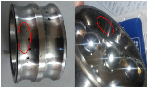
The rolling element bearing (REB) is employed in numerous industrial applications, and its failure can lead to machinery failure [1, 2]. As a result, defect analysis is required to avoid bearing failure [2, 3]. REB vibration data gives a great deal of information about problems and their fault location [4]. Vibration analysis is often used to detect localized faults in REB [5, 6]. The periodic force effects caused by impulsivity at a particular frequency in the presence of a defect are computed using the shaft speed, sampling frequency, and bearing geometry [2-4]. As a result, periodic impulses are a vital status indication of REBs, and defect diagnosis classifies the bearing characteristic frequencies (BCFs) in most circumstances by assuming the outer race is stationary [4, 5, 7]. Localized flaws appear in bearings at numerous points, such as the inner race (IR), the outer race (OR), and the ball and cage [8]. Figure 1 depicts the systematic pattern of inner race faults. The four fundamental frequencies represent different defect sites. The first is ball pass frequency outer race (BPFO), followed by ball pass frequency inner race (BPFI), fundamental train frequency (FTF), and ball spin frequency (BSF). The following are the formulas for specific distinctive frequencies [9]:
$F T F=f_g=\frac{1}{2}\left[f_i\left(1-\frac{d \cos \alpha}{P D}\right)\right]$ (1)
$B S F=f_r=\frac{D_p}{2 d}\left(f_i\right)\left[1-\left(\frac{d \cos \alpha}{P D}\right)^2\right]$ (2)
$B P F I=\left\{\frac{N}{2}\left[f_i\left(1+\frac{d \cos \alpha}{P D}\right)\right]\right\}$ (3)
$B P F O=\left\{\frac{N}{2}\left[f_i\left(1-\frac{d \cos \alpha}{P D}\right)\right]\right\}$ (4)
where, N is the number of rolling elements, PD or Dp is the bearing pitch diameter, ball diameter (d), contact angle (α), and the shaft speed (fi).
Figure 1. Bearing with a cracked inner race
The vibration signals non-linear variables of REB with defects, particularly clearance, friction, and rigidity, indicate non-linear characteristics [9]. As a result, traditional time-domain and frequency-domain signal processing methodologies and advanced signal processing are based on linear structures. Also, the wavelet transformation cannot accurately evaluate REB operating conditions. The growth of non-linear dynamic estimating parameters presents an excellent alternative to understanding and predicting complex non-linear dynamics performance. The parameters based on entropy can define the non-linear dynamic vibration signal features in the time domain, which were studied and applied to diagnosing bearing faults [10]. Pincus [11] has contributed approximate entropy (ApEn), a signal complexity metric utilized in cardiovascular clinical data series. While approximate entropy was adopted and picked as a mechanism for vibration signal handling, it is attributable to its self-adjusting problem. The length of the record has a significant impact on the approximation entropy. For short recordings, the approximation entropy value is continuously lower than predicted and lacks comparative coherence considerably [12]. Richman and Moorman revealed a novel signal complexity metric to address the flaws in approximation entropy [12]. The sample entropy (SampEn) depends on the small data length. Sample entropy is used to diagnose heart rate variability [13]. Still, there is an increased entropy, but it does not necessarily mean that increased entropy correlated with the entropy rise in dynamic complexity [14]. Costa et al. suggested a multi-scale entropy (MSE) system for processing distinct signals on different time scales and utilized analysis of MSE for various physiological data to solve this problem [14, 15]. The utilization of multiple oscillatory modes of vibration signal measurement by Zhang et al. [16] considered mechanical machinery with diverse components and the interaction effects between these components.
The hierarchical entropy (HE) approach was developed using hierarchical decay and entropy analysis to evaluate the complexity of the time series [17]. The HE method is used for the cardiac interval time series to classify numerous heart failures. Considering the lower frequency at each time scale component and the higher frequency generated by averaging the element by computing the difference between two succeeding scales. MSE performs better than HE [17]. Bearing vibration signals have high signal complexity. The fault information is either masked in the lower frequency component or both (Low and High-frequency component), from Low-frequency component interaction effects and mating part effects of various types generated. It emphasizes low-frequency components time series scales, which may not be optimal for obtaining defect characteristics from faulty REB vibration data. Based on this impression, the HE technique is employed to identify roller-bearing problems in the current investigation.
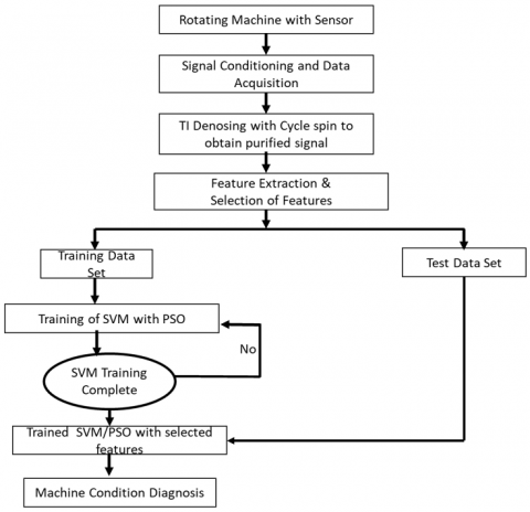
In most cases, the roller bearing defect detection procedure necessitates data collection, feature extraction, and Pattern Recognition [18]. Then traditional artificial neural network (ANN) approaches are examined to investigate whether appropriate samples are available. Support Vector Machines (SVM) is a supervised learning method, and SVM is applied to interpret classification and regression issues such as support vector classification (SVC) and support vector regression (SVR). The smaller sample sizes in specialization theory have a greater conception and guarantee than ANN. The optimal local and global solution is precisely the right [19, 20]. A minimum number of samples will be used by SVM to address the learning issue. It is difficult, or even unlikely, to obtain adequate defect samples for functional uses. As a result of its high precision and generalization, SVM is used to identify faults in rotating machinery. For a more significant number of samples, research [21-23] also attempted to use SVM to classify the rotating unit conditions. The method described in this paper demonstrates how to implement HE and SVM with a particle swarm optimization algorithm for rolling-element bearing with noisy vibration signals. Then, HEs are calculated using sample entropy (SampEn) of eight nodes of hierarchical decomposition to create fault vectors incorporating defect information. In the next step, the defect input characteristics to the SVM Multi-Class Classifier, the defect forms of roller bearings, and varying degrees of severity are marked. Figure 2 represents the flow chart of a hybrid method of TI denoising, HE, and SVM using PSO for fault diagnosis of REB.
Figure 2. Flow chart of the diagnostic procedure
2.1 Introduction TI with cyclic spin denoising
Sometimes, traditional wavelet denoising displays the Gibbs phenomenon visual artifacts [24]. To overcome these artifacts, cyclic spinning is a better choice, where the REB vibration signal data is to be denoised and diverse time shifts translation. Experimentally, cyclic-spinning decreases the root mean square error (RMSE) compared with traditional denoising [24]. In contrast, the wavelet transform is not time-invariant, but cycle spinning has periodic time-invariance. Calculate multiple estimates of the unidentified signal using various shifts and then linearly average the calculations [6, 24]. The process of a cyclic spin is reviewed as follows:
Assume signal $y_{(t)}(0 \leq t \leq n)$ and by introducing the operator of time-shift $S_h . S_h$ represents the circulant shift by h, $\left(S_h y\right)_t=y_{(t+h) \bmod n}$ where mod denotes modulus after division. Timeshift operator is invertible and unitary; therefore, h, $\left(S_h y\right)_t=y_{(t+h) \bmod n}$. The principles of shifting are to remove visual artifacts in terms of this operator and provide an investigation method T, measure instead of T, the time-shifted variant $\hat{T}\left(y ; S_h\right)=S_{-h}\left(T\left(S_h(y)\right)\right)$. The strategy for taking the shift parameter is optimization. Generally, a vibration signal contains discontinuity, which is likely to interfere with one another. Sometimes, the best shift for the first discontinuity of signal is the worst shift for the other discontinuity of signal. We applied the range of shifts in the vibration signal and average over the many results for the above-said reason. Therefore, for time shift H is the range of shift, Ave is the average operator, and
$\hat{T}\left(y ; S_h\right)_{(h \in H)}=A v e_{(h \in H)} S_{-h}\left(T\left(S_h(y)\right)\right)$ (5)
In this way, cycle spinning can identify subspaces and calculate the average of denoising projections.
2.2 Simulated (synthetic) signal
Let us assume the simulated (Synthetic) signal is
$y(t)=y_1(t)+y_2(t)$ (6)
$y_1(t)=\sin (2 \pi 15 t)+0.9 \sin (2 \pi 30 t)$ (7)
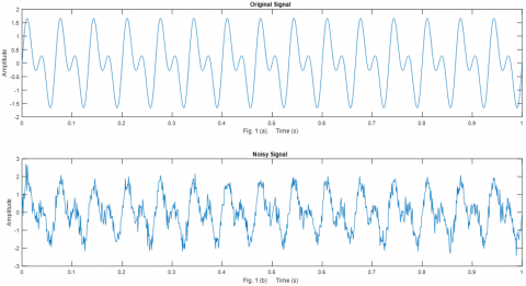
where, y1(t) represents the original signal combining two harmonic waves and, Gaussian noise y2(t), with SNR = 10 dB. The time-domain signal $y_1(t)$ and time-domain signal y(t) Figures 3 (a) and 3(b) are represented, respectively. Assume that the sampling frequency is 1024 Hz, and the sample points are 1024. Figure 3(b) indicates that the original signal $y_1(t)$ is associated with random noise.
In the simulated (synthetic) signal y(t), the Daubechies least symmetric wavelet is considered with four vanishing moments, symmetric wavelet (symN); where N = number of vanishing moments. Cyclic spinning with 15 shifts. The seven shifts to the left and seven to the right, including one zero-shifted signal. The denoising signal results obtained by the cyclic spinning denoising algorithm are represented in Figure 4(a), and the standard orthogonal denoising algorithm is displayed in Figure 4(b), respectively. In the context of projections, this work implemented the cycle spinning method for denoising.
The approximate error obtained by standard orthogonal denoising is 4.2729, and the approximate error obtained by cyclic spinning denoising is 3.4248. Therefore, cyclic spinning denoising is the most suitable alternative for signal denoising and has reduced the approximation error with only 15 shifts.
Figure 3. The time-domain representation. (a) Original or raw signal $y_1(t)$ (b) noisy signal y(t)
Figure 4. Comparison of denoising results on the noisy signal obtained by the cyclic spinning denoising algorithm and the standard orthogonal denoising algorithm. (a) Cyclic spinning denoising (b) standard orthogonal denoising
Sample Entropy (SampEn) is a complexity function like approximate entropy (ApEn). However, it does not contain self-similar patterns as ApEn does. As a statistic, SampEn $(m, r, N)$ is based on three criteria. The first $(m)$ defines the length of the vectors to be used for analysis; the second $(r)$ defines tolerance typically was chosen as a standard deviation factor (SD), and the third (N) represents the data points, respectively. The $N$ data points $\{u(j): 1 \leq j \leq N\}$, form the $N-m+1$ vectors $x_m(i)$ for $\{i \mid 1 \leq i \leq N-m+1\}$ where $x_m(i)=\{u(i+k): 0 \leq k \leq m-1\}$ is the vector of $m$ data points from $u(i)$ to $u(i+m-1)$. The difference between two vectors suggested $d\left[x_m(i), x_m(k)\right]$, is defined as to be $\max \{|u(i+j)-u(k+j)|: 0 j \leq m-1\}$, Maximum variance between their respective scalar elements. The initial formulation of SampEn was watched closely by the Grassberger Procaccia- Integral correlation. However, it is more natural and less notational. The intensive method considers that $\operatorname{SampEn}(\mathrm{m}, \mathrm{r}, \mathrm{N})$ is a negative natural logarithm of the empiric probability that $d\left[x_{m+1}(i), x_{m+1}(k)\right] \leq r$ in terms of the $d\left[x_m(i), x_m(k)\right] \leq r$. Where the values for the parameters are designated and let $\mathrm{B}$ denote the number of pairs $x_m(i) x_m(k)$ such that $\left.d\left[x_m(i), x_m(i)\right)\right] \leq r$, and let A be the number of pairs of vectors $x_{m+1}(i), x_{m+1}(k)$ such that $d\left[x_{m+1}(i), x_{m+1}(k)\right] \leq r$. Then $\operatorname{SampEn}(m, r, N)=$ $-\ln (B / A)$. For convenience, we apply to the combination of two vectors of length $m$. Then match the prototype and compare the length of two vectors $m+1$. SampEn is an ApEn refining approach to determine the complexity of the time series data.
While SampEn has the benefit that it is limited and reliant on the duration of the time sequence, it assigns greater entropy to uncorrelated random white noise signals. Because of this, SampEn's Entropy is higher for uncorrelated random white noise signals. Using the MSE technique, one may create sequential coarse-grained time series $\left\{y^{(\tau)}(j)\right\}$ using the same time series stated before. The following is the equation [14]:
$y^{(\tau)}(j)=\frac{1}{\tau} \sum_{i=(j-1) \tau+1}^{j \tau} x(i)$ (8)
where, scale factor $\tau$ with range$\{1 \leq j \leq N / \tau\}$.
In this section, the physiological system complexity estimation using the HE technique. On the other hand, the multi-scale entropy technique emphasizes the lower frequency components while ignoring the higher frequency component's characteristics. Furthermore, using only lower frequency components will not recreate the original time series—all time-series data collected on a multi-scale basis either in lower or higher frequency components, or both. Multi-scale entropy tests the convolution extremely fit for these entities—this information is primarily preserved in its lower frequency components in time series. However, a high-frequency component will be missing from the data processed. This realization leads to the construction of a hierarchical entropy technique.
We are now applying the approach of hierarchical entropy (HE). We define the average operator $Q_o$ for the time series $(x)=\{x(1), \ldots, x(i), \ldots, x(N)\}$
$Q o(x)=\frac{x(2 j)+x(2 j+1)}{2} \quad j=0,1,2, \ldots, 2^{n-1}$ (9)
The time series $Q o(x)$ with a duration of $2^{n-1}$ is the lowfrequency feature of $(x)$ at scale 2 . The operator of the difference $Q_1$ for the time series $(x)$ is given by
$Q_1(x)=\frac{x(2 j)-x(2 j+1)}{2} \quad j=0,1,2, \ldots, 2^{n-1}$ (10)
The time series $Q_1(x)$ with a length of $2^{n-1}$ is a highfrequency Component of $(x)$ on scale 2 . As an incorporation of this, the time series $Q o(x)$ and $Q_1(x)$ are two-scale timeseries investigations of the $(x)$. For $j=0$ or $1, Q_j$ operators have a matrix representation:
$Q_j=\left[\begin{array}{ccccc}\frac{1}{2} & \frac{(-1)^j}{2} & 0 & 0 & \cdots & 0 & 0\\ 0 & 0 & \frac{1}{2} & \frac{(-1)^j}{2} & \cdots & 0 & 0 \\ 0 & 0 & 0 & 0 & \cdots & \frac{1}{2} & \frac{(-1)^j}{2}\end{array}\right]_{2^{n-1} X 2^n}$ (11)
In the time series, the operator matrix shape depends on the length of the operation. These operators are repetitively used to construct a multi-scale time analysis series(x). For example, suppose that N is a positive integer for $n \in N$ and $\left[v_1, v_2, \ldots \ldots v_n\right] \in\{0,1\}$, the integer
$e=\sum_{j=1}^n v_j 2^{n-1}$ (12)
When $n \in N$ is fixed, the non-negative integer e is a unique vector $\left[v_1, v_2, \ldots, v_n\right]$ which corresponds to it by Eq. (9). The hierarchical components of a time series (x) are defined by
$x_{n, e}=Q_{v_1}, Q_{v_2}, \ldots, Q_{v_n}(x)$ (13)
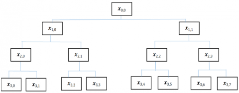
Observation reveals $x_{n, 0}$ represents the low-frequency element of the time series $(x)$ in scale $(n+1)$, whereas $x_{n, 1}$ represents the equivalent high-frequency component. The initial time series $(x)$ is $\left(x_{0,0}\right)$. The signal $\left(x_{n, e}\right)$ is the hierarchical decomposition of signal $(x)$ at different scales for distinct $(n)$ and $(e)$. When $\left\{\tau=2^n\right\}$, the node $\left(x_{n, 0}\right)$ of hierarchical decomposition is the identical to the time series $\left\{y^{(\tau)}\right\}$ of MSE investigation. The hierarchical tree of the hierarchical decomposition of four scales is shown in Figure 5.
Figure 5. Signal (x) four scales hierarchical decomposition
Lastly, the SampEn of each $\left(x_{n, e}\right)$ component is determined and applied to calculate the complexity of the REB Signals. This method is called hierarchical entropy investigation. SamplEn depends strongly on parameters $(m)$ and $(r)$. As a result, the choice of these two constraints is critical. The selection is as detects: $(m=2)$ and {r=0.2$\times$std(standard Deviation)} and of time series, founded on preceding investigations [12]. Assuming that SampEn is not accountable for the data length, the accepted calculation is N=2048.
5.1 Multi-class SVM
The REB defect identification is a classification of several levels that consider different types of faults and varying levels of severity. (One-against-all) and (One-against-one) typical strategies for the multi-class category. According to Hsu and Lin, one-on-one is a conclusive strategy [25]. Consequently, the one-against-one approach is selected here. If $k$ is the number of classes, then $k(k-1) / 2$ is formed as classifiers. Each of them trained on data from two classes. We solve the training data of the $i^{t h}$ and $j^{t h}$ groups. The following two-tier classification problem:
$\operatorname{minimize}: \frac{1}{2}\left\|\omega^{i j}\right\|^2+C \sum_t \xi_t^{i j}\left(\omega^{i j}\right)^T$ (14)
subject to:
$\left(\omega^{i j}\right)^T \phi\left(x_t\right)+b^{i j} \geq 1-\xi_t^{i j}$, if $x_t$ in the ith class, (15)
$\left(\omega^{i j}\right)^T \phi\left(x_t\right)+b^{i j} \geq-1+\xi_t^{i j}$, if $x_t$ in the jth class, (16)
The Max Win Strategy [26] classification is introduced as follows: if Sign $\left(\omega^{i j}\right)^T \phi\left(x_t\right)+b^{i j}$ states that $x$ is in the $i^{\text {th }}$ class of voting for one applied to the $i^{\text {th }}$ class. Otherwise, the $j^{t h}$ would be expanded by one of them. Then $x$ is assigned to the class with the highest numeral of positive majority opinions. The radial base function (RBF) of the kernel is rational. Primary preference and description of the functional implementation of SVM as
$K\left(x_i, x_j\right)=\exp \left(-\Upsilon\left\|x_i-x_j\right\|^2\right)$ (17)
Two parameters appear in the definition for classifying defects: kernel and parameter penalty ϒ and C, respectively.
5.2 Parameters preference with PSO
Particle Swarm Optimization (PSO) is advanced computing. Kennedy 1995 [27, 28] proposed the PSO procedure. And are inspirited by the communal element conduct of a bird assembling. PSO centered on an algorithm for the actions of the assemblage swarm. The algorithm looks for the Optimum value by exchanging cognitive and social knowledge among the particles in the solution space because of its fast convergence property of easy implementation with favorable outcomes [29]. This study combines PSO with k-fold cross-validation to achieve parameter preference of SVM classifier [30].
For the sake of simplicity, this article does not address the PSO algorithm, which is widely available in a lot of literature [29]. For the conventional PSO, the following equations are utilized.
$v_{i j}(t+1)=w v_{i j}(t)+c_1 r_1\left(\right.$ pbest $\left._{i j}-x_{i j}(t)\right)+c_2 r_2\left(\right.$ gbest $\left._j-x_{i j}(t)\right)$ (18)
$x_{i j}(t+1)=x_{i j}(t)+v_{i j}(t+1)$ (19)
where, $v_i(t)$ is the $i t h$ particle velocity at the $t t h$ iteration; pbest $_i(t)$ is termed as the particle's best location; Also the $\operatorname{gbest}_i(t)$ represents the global best location amongst all particles.
In this article, the size of population (swarm size) $p=20$, the inertia weight $w=1$, personal acceleration coefficient $c_1=2$, social acceleration coefficient $c_2=2$, the maximum number of iteration $t_{\max }=200$ are selected respectively. The cross-validation fold number is $k=5$, and the search range of $\Upsilon$ and $C$ is $\left[10^{-2}, 10^{+2}\right]$. The PSO optimization of SVM parameters is divided into the following steps:
Stage 1: Initialization. To every particle (equivalent to c and C of the particle of Variables SVM), build the original location and velocity arbitrarily. Set $p, w, c 1, c 2, t_{\max }$.
Stage 2: Fitness assessment. Find the fitness values for t = 1. A rating SVM classifier with k-fold cross-validation considering fit has a high overall consistency: several previous studies suggest that a high health degree value predicts a lower probability of classification inaccuracy.
Stage 3: Changes. The velocity and location of each are updated using particle-based Eqns. (18) and (19).
Stage 4: Stop it. If the predefined $t_{\max }$ has been reached, execute stage 6.
Stage 5: set the vector iteration: t= t+1 and move to Step 2.
Stage 6: Yield the optimum parameters value of ϒ and C.
6.1 Experimental setup
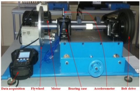
The current manuscript experimented with the SKF test setup to collect vibration signatures for stable and distinct types of defective bearings. The investigation rig comprises a 1 HP induction engine to allow variable speed up to 2900 rpm, as seen in Figure 6. The accelerometer was attached to a rigid bearing housing. In this case, self-aligned ball bearings are used for investigation purposes. Table 1 displays the particulars of the experimental bearing used during the investigation and the working condition of the test bearing-the defects produced on various bearing components utilizing an electrical discharge drill. Table 2 displays the characteristic frequencies of REB used, and Table 3 shows the rolling element bearing parameters. Baseline data was collected by running a healthy bearing in the investigation rig. Then, the various faulty, defective information was obtained using the SKF GX Series Microlog CMXA-75 (Handheld FFT analyzer).
Defects considered for the current work as presented in Figure 7. In this inquiry, the subsequent four classes of REB conditions are classified. Time series vibration data were registered at 820 rpm and 1500 rpm for normal and faulty bearings. The sampling rate used to capture the vibration information was 6.4 kHz, and the REB vibration data were recorded and captured for 5 seconds. Periodic and low amplitude peaks are associated with healthy bearings, whereas the higher magnitude of non-periodic peaks must be noticeable for IR defects.
Figure 6. Experimental setup
Figure 7. Defects (a) Inner race fault, (b) Outer race fault
The ball and outer race defects identified low and intermittent amplitude vibration behavior. However, such behavior was not detected by the time domain vibration signal. These time-domain vibration signals show non-stationary behavior. Thus, these signals have been analyzed using a non-stationary signal processing technique which is part of this work.
6.2 Results and analysis
To demonstrate the suggested procedure for the experimental findings from the above tests is used to test a roller bearing defect diagnostic. Table 4 to Table 12 shows test REB vibration data from four distinct circumstances, including healthy bearing data, bearings with IR defects, OR defects, ball defects, and varying degrees of severity for individual defects. In Figure 10 and Table 4, a ten-class issue emerged from the experimental investigation due to the multiple faults and their proportions. The experimental data contains 400 samples, with 820 rpm sample data abbreviated to a 2048-point time series and 1500 rpm sample data to a 4096-point time series. In addition, none of them overlapped the 400 vibration sample data. One hundred samples are randomly picked for training data, while the remaining 300 are for test data to create the model.
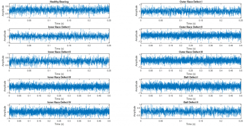
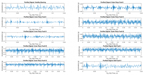
A total of Ten different bearing conditions (Healthy bearing, IR defect, OR defect, and ball defect) time-domain original signal was obtained from the test bearing, as shown in Figure 8. Figure 8 displays that the impact part is obscured by ambient noise due to the fault that exists in the rolling bearing and noise due to the experimental test setup associated component. Apply the translation-invariant wavelet denoising and obtain the purified signal Figure 9. The background noise present in the different bearing conditions is effectively suppressed.
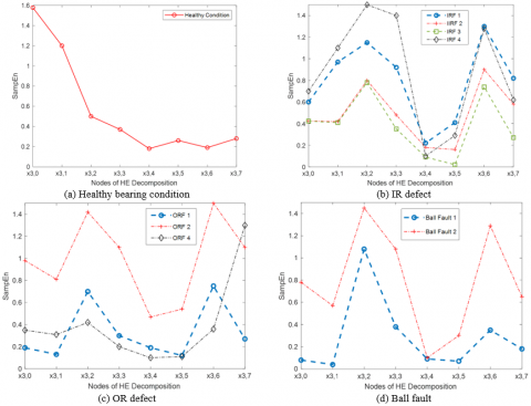
As a result of this experiment, the vibration signal test data is three times as large as the training data in this study. The original time-domain signal of 10 bearing circumstances is represented in Figure 8, and the purified time-domain signal of the corresponding ten bearing conditions is illustrated in Figure 9. The SampEn of eight nodes of HE decomposition for ten purified time-domain waveform bearing conditions is represented in Figure 10. It is apparent in Figure 10 that when the HE of the healthy bearing increases, the low-frequency components become more dominant. However, bearings with IR faults, OR faults, and ball faults have a high-frequency value in both frequency regions. This guarantees that, under healthy situations, the system on vibration signals is generally preserved in its low-frequency components. When no fault is present, the majority opinion is supported by evidence that no high-frequency impulse is generated. It can be observed that distinct defective situations have different HE values, even though the corresponding HE values follow a similar pattern.
Table 1. Working condition of the experimental REB
|
|
REB Model |
Motor load |
Fault characterization |
Speed (rpm) |
REB Condition |
|
Case Study 1 |
2207EKTN9 |
0-1 HP |
Diameter: 0.18, 0.53 & 1mm |
1500 |
Ball defect |
|
|
|
|
Depth: 0.2mm |
820 |
IR defect |
|
|
|
|
|
(IR & OR) |
OR defect |
|
|
|
|
|
Depth: 0.1 mm (Ball Fault) |
(Centered @ 6:00) |
Table 2. Characteristic frequencies of REB
|
Characteristic frequencies (Hz) |
Shaft Frequency |
FTF |
BSF |
BPFI |
BPFO |
|
Case Study 1 |
25 |
9.81 |
55.5 |
182 |
117.81 |
|
|
13.66 |
5.36 |
30.37 |
99.55 |
64.37 |
Table 3. REB parameters
|
|
Number of ball N |
Angle of contact α |
Ball diameter d |
Outside Diameter |
Inside Diameter |
Pitch Diameter Dp |
|
Case Study 1 |
9 |
0 |
7.9 |
52 |
25 |
46.4 |
Figure 8. Ten various bearing conditions time-domain waveform
Figure 9. Ten various bearing conditions purified the time-domain waveform
Figure 10. The eight nodes in hierarchical decomposition and their HE values under the following ten bearing conditions
By referring to Figure 10, the HE is suitable for usage as an indicator of faulty features, as it deviates from each other HE. Following the extraction of HE as Feature vectors produced from training and test data, respectively. Test data characteristic vectors are divided into a training set and a test set, each with 100 samples.
As designated in Section $4.2$, the PSO technique is coupled through Cross-validation to produce the optimum Penalty parameter $C$, kernel parameter $\Upsilon$, and Training method, resulting in optimal $C=0.1000$ and $\Upsilon=9.8337$. A multi-class SVM classifier uses the training set to create a forecast model. After that, the testing data set is fed into the trained model, then the various defect configurations and severity of REB are reported.
No misclassified samples were under any of the ten bearing situations, as shown in Table 5. Indicate that both the test and the training are 100 percent accurate. To demonstrate the advantages of TI denoising with HE in this study, MSEs were computed over eight scales of the sample data to create characteristic vectors toward observation. Optimal and $\Upsilon=$ $7.4838$ are found using the same approach described previously.
According to Table 6, eight samples were miscategorized throughout the test data collection, and the overall test efficiency is 97.3 percent. The investigation recommends HE will be able to extract both low- and high-frequency findings. The suggested TI denoising using the HE technique is predominant to the MSE technique for categorizing various REB circumstances. To better illustrate the performance and dominance of HE as defect characteristics, an ANN has a weaker simplification than SVM in the event of a short quantity of data to comprehensively detect ten distinct defect configurations. A frequently used backpropagation (BP) algorithm for ANN preparation is utilized. The input layer, output layer, and hidden layer/s are the three layers that make up an ANN.
The input layer receives the data from the network and stores it in a database. As the essential information is obtained from the input layer, it is processed by the hidden layer. It is then transferred to the output layer, which will also analyze the information from the hidden layer and provide the output. The number of the feature vector is used to determine the input layer node number. The input number of layer nodes is 8, whereas the number of output nodes is 10, and the number of defect categories calculates it. Three types of node number of hidden layers arbitrarily endeavored in this article, which is 18, 20, and 22, respectively.
Table 4. Experiment group 1: The proposed method for different cases is constructed by variations of type (IRF, ORF, and REF), size (Slight, Moderate and Severe), speed rpm (820 and 1500), and load (0 hp and 1 hp) of fault bearings
|
Fault Class |
Fault Size (mm) |
Fault Severity |
Load (hp) |
RPM |
Number of Training data |
Number of Testing data |
Class Label |
Number of Misclassified Samples |
Wrong output of testing data |
Recognition rate |
|
Normal |
0 |
----- |
0 |
1500 |
10 |
30 |
1 |
0 |
0 |
100% |
|
IRF |
0.18 |
Slight |
0 |
820 |
10 |
30 |
2 |
0 |
0 |
100% |
|
|
0.53 |
Moderate |
1 |
820 |
10 |
30 |
3 |
0 |
0 |
100% |
|
|
1.00 |
Severe |
1 |
1500 |
10 |
30 |
4 |
0 |
0 |
100% |
|
|
0.18 |
|
0 |
1500 |
10 |
30 |
5 |
0 |
0 |
100% |
|
ORF |
0.18 |
|
0 |
820 |
10 |
30 |
6 |
0 |
0 |
100% |
|
|
0.53 |
|
1 |
1500 |
10 |
30 |
7 |
0 |
0 |
100% |
|
|
1.00 |
|
1 |
1500 |
10 |
30 |
8 |
0 |
0 |
100% |
|
REF |
0.18 |
|
0 |
820 |
10 |
30 |
9 |
0 |
0 |
100% |
|
|
0.53 |
|
1 |
1500 |
10 |
30 |
10 |
0 |
0 |
100% |
|
In Total |
|
|
|
|
100 |
300 |
|
0 |
0 |
100% |
Table 5. Experiment group 1: The results of the recognition are based on MSE and SVM for different cases are constructed by variations of type, size, speed rpm, and a load
|
Fault Class |
Fault Size (mm) |
Fault Severity |
Load (hp) |
RPM |
Number of Training data |
Number of Testing data |
Class Label |
Number of Misclassified Samples |
Wrong output of testing data |
Recognition rate |
|
Normal |
0 |
----- |
0 |
1500 |
10 |
30 |
1 |
0 |
0 |
100% |
|
IRF |
0.18 |
Slight |
0 |
820 |
10 |
30 |
2 |
0 |
0 |
100% |
|
|
0.53 |
Moderate |
1 |
820 |
10 |
30 |
3 |
0 |
0 |
100% |
|
|
1.00 |
Severe |
1 |
1500 |
10 |
30 |
4 |
0 |
0 |
100% |
|
|
0.18 |
|
0 |
1500 |
10 |
30 |
5 |
0 |
0 |
100% |
|
ORF |
0.18 |
|
0 |
820 |
10 |
30 |
6 |
0 |
0 |
100% |
|
|
0.53 |
|
1 |
1500 |
10 |
30 |
7 |
0 |
1 |
96.6% |
|
|
1.00 |
|
1 |
1500 |
10 |
30 |
8 |
0 |
2 |
93.3% |
|
REF |
0.18 |
|
0 |
820 |
10 |
30 |
9 |
0 |
4 |
86.6% |
|
|
0.53 |
|
1 |
1500 |
10 |
30 |
10 |
0 |
0 |
100% |
|
In Total |
|
|
|
|
100 |
300 |
|
0 |
8 |
97.3% |
Table 6. Experiment group 2: The second cluster of an experiment for Defect type identification with the same defect severity, different fault types, and the same load
|
Fault Severity (mm) |
Load (hp) |
Number of Categories |
Number of Training data |
Number of Testing data |
Recognition rate |
RPM |
Variance |
|
0.18 (Slight) |
0 |
03 (IRF, ORF & REF) |
10 |
30 |
100% |
820 |
0 |
|
|
1 |
03 |
10 |
30 |
100% |
820 |
0 |
|
0.53 (Moderate) |
0 |
03 |
10 |
30 |
100% |
820 |
0 |
|
|
1 |
03 |
10 |
30 |
100% |
820 |
0 |
|
1.00 (Severe) |
0 |
03 |
10 |
30 |
97.66% |
820 |
0.12 |
|
|
1 |
03 |
10 |
30 |
98.32% |
820 |
0.30 |
|
0.18 |
0 |
03 |
10 |
30 |
100% |
1500 |
0 |
|
|
1 |
03 |
10 |
30 |
100% |
1500 |
0 |
|
0.53 |
0 |
03 |
10 |
30 |
100% |
1500 |
0 |
|
|
1 |
03 |
10 |
30 |
100% |
1500 |
0 |
|
1.00 |
0 |
03 |
10 |
30 |
99.88% |
1500 |
0.32 |
|
|
1 |
03 |
10 |
30 |
99.77% |
1500 |
0.23 |
Table 7. Experiment group 3: Defect type identification with similar defect severity, different fault types (IRF, ORF, and REF), and the additional loading (0 hp and 1 hp)
|
Fault Severity (mm) |
Number of sample |
Number of Categories |
Number of Training data |
Number of Testing data |
Recognition rate |
RPM (hp) |
Load |
Variance |
|
0.18 (Slight) |
100 |
03 (IRF, ORF & REF) |
40 |
60 |
100% |
820 |
0 |
0 |
|
0.53 (Moderate) |
100 |
03 |
40 |
60 |
100% |
820 |
0 |
0 |
|
1.00 (Severe) |
50 |
03 |
20 |
30 |
97.46% |
820 |
0 |
0.35 |
|
0.18 |
100 |
03 |
40 |
60 |
100% |
1500 |
1 |
0 |
|
0.53 |
100 |
03 |
40 |
60 |
100% |
1500 |
1 |
0 |
|
1.00 |
50 |
03 |
20 |
30 |
99.52% |
1500 |
1 |
0.31 |
Table 8. Experiment group 4: Defect type identification with different defect types and irrespective of the level of defect severity under a similar load
|
Load (hp) |
Number of sample |
Number of Categories |
Number of Training data |
Number of Testing data |
Recognition rate |
RPM |
Variance |
|
0 |
200 |
03 (IRF, ORF & REF) |
40 |
60 |
99.09% |
820 |
0.10 |
|
1 |
200 |
03 |
40 |
60 |
97.63% |
820 |
0.29 |
Table 9. Experiment group 5: The second cluster of an experiment for the level of defect severity identification with the different levels of defect severity with the same fault type and the same load
|
Fault type |
Load (hp) |
Number of Categories |
Number of Training data |
Number of Testing data |
Recognition rate |
RPM |
Variance |
|
IRF |
0 |
03 (Slight, Medium & Severe) |
40 |
60 |
99.92% |
820 |
0.28 |
|
ORF |
|
03 |
40 |
60 |
100 |
820 |
0 |
|
REF |
|
03 |
40 |
60 |
100 |
820 |
0 |
|
IRF |
1 |
03 (Slight, Medium & Severe) |
40 |
60 |
99.11% |
820 |
0.24 |
|
ORF |
|
03 |
40 |
60 |
100 |
820 |
0 |
|
REF |
|
03 |
40 |
60 |
99.56% |
820 |
0.81 |
|
IRF |
0 |
03 (Slight, Medium & Severe) |
40 |
60 |
100% |
1500 |
0 |
|
ORF |
|
03 |
40 |
60 |
100 |
1500 |
0 |
|
REF |
|
03 |
40 |
60 |
99.46 |
1500 |
0.66 |
|
IRF |
1 |
03 (Slight, Medium & Severe) |
40 |
60 |
99.81% |
1500 |
0.07 |
|
ORF |
|
03 |
40 |
60 |
100 |
1500 |
0 |
|
REF |
|
03 |
40 |
60 |
99.23% |
1500 |
0.19 |
Table 10. Experiment group 6: The second cluster of an experiment for the level of defect severity identification with the different levels of defect severity with the same fault type and irrespective of the load
|
Fault type |
Number of Categories |
Total Number of Sample |
Number of Training data |
Number of Testing data |
Recognition rate |
Variance |
|
IRF |
03 (Slight, Medium & Severe) |
180 |
80 |
100 |
99.35% |
0.28 |
|
ORF |
03 |
180 |
80 |
100 |
99.70% |
0 |
|
REF |
03 |
180 |
80 |
100 |
99.20% |
0 |
Table 11. Experiment group 7: Eight malfunctioning working conditions with different fault types and different levels of defect severity under a similar load (0 hp and 1 hp)
|
Load (hp) |
Number of Sample |
Categories |
Total Number of Sample |
Number of training data |
Number of Testing data |
Recognition rate |
Variance |
|
0 |
200 |
08 |
100 |
40 |
60 |
99.12% |
0.17 |
|
1 |
200 |
08 |
100 |
40 |
60 |
98.88% |
0.15 |
|
(Categories 08: IRF, ORF and REF, Slight, Moderate and Severe, 0 hp and 1 hp) |
|||||||
Table 12. Experiment group 7: Regardless of the load, there are eight faulty operating circumstances with distinct fault kinds and varying levels of defect severity
|
Categories |
Total Number of Sample |
Number of training data |
Number of Testing data |
Recognition rate |
Variance |
|
11 |
600 |
200 |
400 |
98.02% |
0.13 |
|
(Categories 08: IRF, ORF and REF, Slight, Moderate and Severe, 0 hp and 1 hp) |
|||||
Table 13. Assessment of the suggested method's average testing accuracy and variance with MSE-ICDSVM, IMFPE-SFNN, IMFPE-SVM, and IMFPE-RBFNN
|
Load (hp) |
Average testing accuracy |
IMFPE-SFNN/ Variance |
IMFPE – RBFNN/Variance |
MSE-ICDSVM/Variance |
IMFPE-SVM/Variance |
Proposed method/Variance |
|
0 |
|
95.63% |
95.85% |
96.88% |
81.33% |
99.12% |
|
|
|
95.63% |
95.85% |
96.88% |
81.33% |
99.12% |
|
1 |
|
96.22% |
96.18% |
98.56% |
83.21% |
98.88% |
|
|
|
0.98 |
0.72 |
0.75 |
0.89 |
0.15 |
|
Irrespective of the load |
|
95.15% |
95.56% |
96.50% |
80.87% |
98.02% |
|
|
0.55 |
0.32 |
0.68 |
0.65 |
0.13 |
Table 14. To classify fault types and fault severity and this current research was compared to existing literature
|
Source |
Characteristic features |
Classifier |
Defect considered |
Number of classified states |
Classification Rate |
Observations |
|
[31] |
(LCD) + fuzzy entropy (ANFIS) |
(ANFIS) |
N, B (0.1778, 0.5334 mm), IR (0.1778, 0.5334 mm), OR (0.1778, 0.5334 mm), |
7 |
100 |
|
|
[32] |
Frequency and Time-domain features |
Multi-staged decision algorithm based on ANN and (ANFIS) |
N, IR (0.3, 0.6, 1, 2 mm) OR (0.3, 0.6, 1, 2 mm) |
9 |
|
ANN: 89-100 for each condition ANFIS: 92-100 for each condition |
|
[33] |
Lempel–Ziv complexity Quantitative based on CWT, EMD, analysis Wavelet packet transform, Entropy, Kurtosis |
NA |
IR (0.5, 2, 3.5, 5 mm) OR (0.5, 2, 3.5, 5 mm) |
8 |
|
NA |
|
Current Work |
TI, HE and SVM |
HE/SVM with PSO with PSO optimization algorithm |
IR (0.18, 0.53, 1 mm) OR (0.18, 0.53, 1 mm) |
3,8,11 |
98.67-100 |
Normal condition detect rate 100% |
The results of the ANN recognition indicate the utility and applicability of TI denoising and the HE method as a function of REB fault analysis. Correspondingly, each pattern has ten samples that are used to train the ANN. Also, the 100 samples are used as training data, while the residual 300 are used as assessment data. The classification accuracy is 100 percent when the trained ANN is applied to the test samples, regardless of the hidden layer's node number.
Similarly, experiment group (3), represented in Table 7, performs the test on defect type identification with similar defect severity (Slight, Moderate, and Severe), different fault types (IRF, ORF, and REF), and additional loading (0 hp and 1 hp). Experiment group (4), represented in Table 8, performs the test on Defect type identification with varying types of the defect (IRF, ORF, and REF) and irrespective of the level of defect severity (Slight, Moderate, and Severe) under a similar load (0 hp and 1 hp). Experiment group (5) Table 9 represents the second cluster of an experiment for the level of defect severity identification with the different levels of defect severity (Slight, Moderate, and Severe) with the same fault type (IRF, ORF, and REF) and the same load (0 hp and 1 hp). Experiment group (6) Table 10, represents the second cluster of an experiment for the level of defect severity identification with the different levels of defect severity (Slight, Moderate, and Severe) with the same fault type (IRF, ORF, and REF) and irrespective of the load (0 hp and 1 hp). Whereas in Table 11 Experiment group 7, the test consists of eight malfunctioning working conditions with different fault types (IRF, ORF, and REF) and different levels of defect severity (Slight, Moderate, and Severe) under a similar load (0 hp and 1 hp). The Table 12 Experiment group 7 test consists of eight malfunctioning working conditions with different fault types (IRF, ORF, and REF) and different levels of defect severity (Slight, Moderate, and Severe) and irrespective of the load (0 hp and 1 hp). Assessment of the suggested method average testing accuracy and variance with MSE-ICDSVM, IMFPE-SFNN, IMFPE-SVM, and IMFPE-RBFNN are represented in Table 13. Table 14 compares the current research with existing literature and indicates a 98.67 to 100 percent classification rate. The recognition results demonstrate the utility and applicability of the TI denoising and HE methods as a function of REB fault analysis.
This article presents a novel hybrid bearing fault detection approach-based TI denoising with HE and SVM using the particle swarm optimization (PSO) method for REB faults detection. The rolling element bearing vibration generally exhibits the effects of mechanical components interaction, which shows non-linear dynamic characteristics. The HEs of REB signals at scale 4 under different conditions establish characteristic defect vectors. These vector features are subsequently input into the SVM to classify the defect. PSO was utilized throughout the SVM prediction model training procedure to customize the SVM of a particular process or activity. The experimental findings have proved to be successful. For reference, an experiment on the classification of fault bearings uses MSE as a fault feature, which shows TI denoising with HE can extract additional fault information than MSE, and the HE approaches will achieve better classification accuracy, up to 100 percent of it. The result recognises that the provided approach for defect investigation is practical for the REB's condition monitoring, despite the limited sample size. Furthermore, the experimental research given here is characterised by a uniform pace. Future research will focus on determining the resilience of the proposed approach in the presence of rotation speed variations. The empirical mode decomposition (EMD) approach is also adaptable and is used for non-stationary signals.
[1] Belkacemi, B., Saad, S., Ghemari, Z., Zaamouche, F., Khazzane, A. (2020). Detection of induction motor improper bearing lubrication by discrete wavelet transforms (DWT) decomposition. Instrumentation Mesure Métrologie, 19(5): 347-354. https://doi.org/10.18280/i2m.190504
[2] Agrawal, P., Jayaswal, P. (2020). Diagnosis and classifications of bearing faults using artificial neural network and support vector machine. Journal of The Institution of Engineers (India): Series C, 101(1): 61-72. https://doi.org/10.1007/s40032-019-00519-9
[3] Jayaswal, P., Wadhwani, A.K., Mulchandani, K.B. (2008). Machine fault signature analysis. International Journal of Rotating Machinery, 2008: 583982. https://doi.org/10.1155/2008/583982
[4] El-Thalji, I., Jantunen, E. (2015). A summary of fault modelling and predictive health monitoring of rolling element bearings. Mechanical Systems and Signal Processing, 60: 252-272. https://doi.org/10.1016/j.ymssp.2015.02.008
[5] Yang, G., Sun, X.B., Zhang, M.X., Li, X.L., Liu, X.R. (2014). Study on ways to restrain end effect of Hilbert-Huang transform. Journal of Computers, 25(3): 22-31. https://doi.org/10.1.1.695.7077
[6] Donoho, D.L. (1995). De-noising by soft-thresholding. IEEE Transactions on Information Theory, 41(3): 613-627. https://doi.org/10.1109/18.382009
[7] Huang, N.E., Wu, Z., Long, S.R., Arnold, K.C., Chen, X., Blank, K. (2009). On instantaneous frequency. Advances in Adaptive Data Analysis, 1(2): 177-229. https://doi.org/10.1142/S1793536909000096
[8] Qin, X., Li, Q., Dong, X., Lv, S. (2017). The fault diagnosis of rolling bearing based on ensemble empirical mode decomposition and random forest. Shock and Vibration, 2017: 2623081. https://doi.org/10.1155/2017/2623081
[9] Yu, Y., Yu, D., Cheng, J. (2006). A roller bearing fault diagnosis method based on EMD energy entropy and ANN. Journal of Sound and Vibration, 294(1-2): 269-277. https://doi.org/10.1016/j.jsv.2005.11.002
[10] Zhang, L., Xiong, G., Liu, H., Zou, H., Guo, W. (2010). Bearing fault diagnosis using multi-scale entropy and adaptive neuro-fuzzy inference. Expert Systems with Applications, 37(8): 6077-6085. https://doi.org/10.1016/j.eswa.2010.02.118
[11] Pincus, S. (1995). Approximate entropy (ApEn) as a complexity measure. Chaos: An Interdisciplinary Journal of Nonlinear Science, 5(1): 110-117. https://doi.org/10.1063/1.166092
[12] Richman, J.S., Moorman, J.R. (2000). Physiological time-series analysis using approximate entropy and sample entropy. American Journal of Physiology-Heart and Circulatory Physiology, 278(6): H2039-H2049. https://doi.org/10.1152/ajpheart.2000.278.6.H2039
[13] Lake, D.E., Richman, J.S., Griffin, M.P., Moorman, J.R. (2002). Sample entropy analysis of neonatal heart rate variability. American Journal of Physiology-Regulatory, Integrative and Comparative Physiology, 283(3): R789-R797. https://doi.org/10.1152/ajpregu.00069.2002
[14] Costa, M., Goldberger, A.L., Peng, C.K. (2002). Multi-scale entropy analysis of physiologic time series. Physical Review Letters, 89: 062102.
[15] Costa, M., Goldberger, A.L., Peng, C.K. (2005). Multiscale entropy analysis of biological signals. Physical Review E, 71(2): 021906. https://doi.org/10.1103/PhysRevE.71.021906
[16] Zhang, L., Xiong, G., Liu, H., Zou, H., Guo, W. (2010). Bearing fault diagnosis using multi-scale entropy and adaptive neuro-fuzzy inference. Expert Systems with Applications, 37(8): 6077-6085. https://doi.org/10.1016/j.eswa.2010.02.118
[17] Jiang, Y., Peng, C.K., Xu, Y. (2011). Hierarchical entropy analysis for biological signals. Journal of Computational and Applied Mathematics, 236(5): 728-742. https://doi.org/10.1016/j.cam.2011.06.007
[18] Yang, Y., Yu, D., Cheng, J. (2007). A fault diagnosis approach for roller bearing based on IMF envelope spectrum and SVM. Measurement, 40(9-10): 943-950. https://doi.org/10.1016/j.measurement.2006.10.010
[19] Zacksenhouse, M., Braun, S., Feldman, M., Sidahmed, M. (2000). Toward helicopter gearbox diagnostics from a small number of examples. Mechanical Systems and Signal Processing, 14(4): 523-543. https://doi.org/10.1006/mssp.2000.1297
[20] Vapnik, V. (1999). The Nature of Statistical Learning Theory. Springer Science & Business Media.
[21] Khelil, J., Khelil, K., Ramdani, M., Boutasseta, N. (2020). Discrete wavelet design for bearing fault diagnosis using particle swarm optimization. Journal Européen des Systèmes Automatisés, 53(5): 705-713. https://doi.org/10.18280/jesa.530513
[22] Abbasion, S., Rafsanjani, A., Farshidianfar, A., Irani, N. (2007). Rolling element bearings multi-fault classification based on the wavelet denoising and support vector machine. Mechanical Systems and Signal Processing, 21(7): 2933-2945. https://doi.org/10.1016/j.ymssp.2007.02.003
[23] Shen, Z., Chen, X., Zhang, X., He, Z. (2012). A novel intelligent gear fault diagnosis model based on EMD and multi-class TSVM. Measurement, 45(1): 30-40. https://doi.org/10.1016/j.measurement.2011.10.008
[24] Coifman, R.R., Donoho, D.L. (1995). Translation-invariant de-noising. In: Antoniadis, A., Oppenheim, G. (eds) Wavelets and Statistics. Lecture Notes in Statistics, vol 103. Springer, New York, NY. https://doi.org/10.1007/978-1-4612-2544-7_9
[25] Hsu, C.W., Lin, C.J. (2002). A comparison of methods for multiclass support vector machines. IEEE transactions on Neural Networks, 13(2): 415-425. https://doi.org/10.1109/72.991427
[26] Widodo, A., Yang, B.S. (2007). Support vector machine in machine condition monitoring and fault diagnosis. Mechanical Systems and Signal Processing, 21(6): 2560-2574. https://doi.org/10.1016/j.ymssp.2006.12.007
[27] Kennedy, J., Eberhart, R. (1995). Particle swarm optimization. In Proceedings of ICNN'95-International Conference on Neural Networks, 4: 1942-1948. https://doi.org/10.1109/ICNN.1995.488968
[28] Kenndy, J., Eberhart, R.C. (1995). A new optimizer using particle swarm theory. Proceedings of the Sixth International Symposium onMicro-Machine and Human Science, pp. 39-43.
[29] Poli, R., Kenndy, J., Blackwell, T. (2007). Particle swarm optimization: An overview. Swarm Intell, 1(1): 33-55.
[30] Hsu, C.W., Chang, C.C., Lin, C.J. (2003). A practical guide to support vector classification. Technical Report, Department of Computer Science and Information Engineering, University of National Taiwan, Taipei, pp. 1-12.
[31] Zheng, J., Cheng, J., Yang, Y. (2013). A rolling bearing fault diagnosis approach based on LCD and fuzzy entropy. Mechanism and Machine Theory, 70: 441-453. https://doi.org/10.1016/j.mechmachtheory.2013.08.014
[32] Ertunc, H.M., Ocak, H., Aliustaoglu, C. (2013). ANN-and ANFIS-based multi-staged decision algorithm for the detection and diagnosis of bearing faults. Neural Computing and Applications, 22(1): 435-446. https://doi.org/10.1007/s00521-012-0912-7
[33] Wang, J., Cui, L., Wang, H., Chen, P. (2013). Improved complexity based on time-frequency analysis in bearing quantitative diagnosis. Advances in Mechanical Engineering, 5: 258506. https://doi.org/10.1155/2013/258506