Lei Feng | Haibin Li* | Defang Cheng | Wenming Zhang | Cunjun Xiao
© 2022 IIETA. This article is published by IIETA and is licensed under the CC BY 4.0 license (http://creativecommons.org/licenses/by/4.0/).
OPEN ACCESS
Visual saliency detection aims to extract salient objects from the original image, making it less complicated to process the image. This paper combines an edge box algorithm with Bayesian theory to detect salient objects. The proposed saliency detection algorithm transforms the process of traditional detection method, and prioritizes the positioning of significant objects. Firstly, the Harris corners of the original image were calculated, and clustered by the improved clustering algorithm, yielding the number of salient objects in the image. Then, all possible positions of salient objects in the image were framed by the edge box algorithm, and the boxes were sorted in descending order of the score. According to the number N of clusters of the image corners, the N top-ranking boxes were selected to determine the salient regions. In this way, the position and number of salient objects were clarified. Based on the selected salient regions, the final saliency map was calculated by improved geodesic distance and Bayesian model. Experimental results show that our approach performed better than 11 existing algorithms in both simple and relatively complex scenes. In terms of objective performance, the accuracy and recall of our algorithm on MSRA10k, ECSSD, DUT-OMRON and SED2 datasets were higher than that of the other algorithms.
saliency detection, edge boxes, Bayesian model
Visual saliency detection relies on the principle of human vision to quickly locate the areas with a high contrast against the surrounding areas. In the human visual system, the special ability of dynamic selection is known as the visual attention mechanism. Through information filtering, this mechanism can filter out the redundant information from the original image, while preserving the regions of interest (ROIs). The filtering enhances the efficiency of image processing, and avoids the waste of computing resources. As a result, more and more researchers start to explore the technology of visual saliency detection, trying to introduce the visual attention mechanism to computers.
The technology of visual saliency detection has long been a key research direction of computer vision in the field of image processing. Among the existing models of visual saliency detection, the bottom-up (data-driven) models aim to extract the underlying features of the original image as salient features (such as color, edge, and corner), and highlight the extracted features by a specific algorithm, while the top-down (task driven) models intend to extract image features through computer learning of specific tasks.
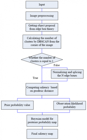
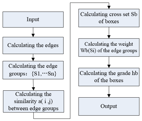
The mainstream visual saliency detection methods face two common problems: the unclear edges of the salient objects, and the difficulty in highlighting the objects uniformly. To overcome the problems, this paper presents a saliency detection method based on edge boxes and Bayesian theory. Firstly, unimportant details of the original images were smoothed through L0 gradient minimization, while preserving the edges of the foreground. The computing load was reduced by super-pixel segmentation. In addition, the Harris algorithm of color enhancement was called to identify the corner points in the image, and remove the edge corner points of non-salient objects. The number of clusters for the corners was calculated by the data clustering algorithm of density-based spatial clustering of applications with noise (DBSCAN), laying the basis for single object or multi-object saliency detection in the image. Furthermore, the edge box algorithm was employed to position each object.
The number of boxes depends on the number of clusters obtained in the previous step. If the number of clusters is 1, there is one salient object in the image. Then, the box with the highest voting score was selected for visual saliency detection. If the number n of clusters is greater than 1, there are N salient objects in the image, corresponding to N boxes. The scores of the boxes were sorted in descending order, and the N top-ranking boxes were selected. The images of these N boxes were spliced and normalized. Finally, the saliencies outside the box were set to 0, and the ultrametric contour map (UCM) value was taken as the edge weight of the super-pixel. Drawing on the concept of geodesic distance, the distance between the super-pixel inside the box and the background seed super-pixel at the box edge was calculated as the prior probability. The color distribution in and out of the box was taken as the observation likelihood probability. Then, the Bayesian formula was used to derive the posterior probability, i.e., the final saliency map. The flow of our algorithm is shown in Figure 1.
The remaining part of this paper is organized as follows: Section 2 reviews different approaches of visual saliency detection; Section 3 details the image preprocessing technique; Section 4 introduces salient corner detection and lustering; Section 5 improves the edge box algorithm; Section 6 applies Bayesian theory in saliency detection; Section 7 illustrates the implementation procedure of our approach; Section 8 displays and evaluates the experimental results; Section 9 summarizes the advantages of our algorithm, and describes the future research directions.
Figure 1. Flow of our algorithm
The ultimate goal of machine vision is to make computer have the ability of human vision system, which is a very challenging task. Thanks to the visual attention mechanism, it is easy for human to recognize the salient objects in the original image, filter out the uninterested information from the noisy background, and retain the ROIs. The core purpose of an image saliency detection algorithm is to reduce the complexity of image processing.
The past two decades have witnessed great progress in visual saliency detection. Many algorithms are developed for various fields, such as cognitive psychology, neuroscience and computer vision. In 1998, Itti et al. [1] put forward the classic bottom-up saliency detection model. Itti’s model tries to detect salient objects by the principle of center-surrounding contrast. The contast is mainly computed around the center, and the saliency is defined based on the low-level features on different scales of the image. This model lays a solid foundation for subsequent visual saliency detection algorithms. In 2007, Hou et al. [2] generated a saliency model by the spectral residual (SR) method. Their model divides image information into a frequent change part and a prior knowledge part. The human visual system pays more attention to the changing scarce information in a scene, and ignores the repeated information.
In 2010, Goferman et al. [3] developed a context-aware (CA) saliency detection algorithm, based on local and global color contrasts. The basic idea of the algorithm is as follows: a highly salient region must be unique. The spatial positions of pixels as considered in the algorithm. Zhu et al. [4] presented a robust background measurement method to measure spatial layout and edge. The method assesses background connectivity to separate the salient objects. Firstly, the connectivity is proposed to calculate the regional contrast, and used to compute the background probability, before derving the background contrast weight. This background measurement method describes the regional background and salient objects well.
Background priori plays a crucial role in salient object detection. Wei et al. [5] designed two background priors, namely, edge priori and continuity priori, and computes the shortest path length from the edge priori to the virtual background node, drawing on the concept of geodesic distance. The shorest path length represents the saliency of image super-pixel. Their attempt alleviates the dependence on the background priori, and prevents the one-dimensional (1D) saliency of image edge solution. Considering global contrast, Cheng et al. created an algorithm based on histogram contrast (HC) and region contrast (RC) [6].
The salient objects can be detected excellently, when the signals are depicted by the sparse theory. Therefore, image saliency detection based on sparse representation has gain popularity. In 2017, Zeng et al. [7] proposed a novel saliency detection algorithm under unsupervised game theory. Firstly, saliency detection is regarded as a non-cooperative game problem, and the revenue function is constructed based on multiple clues and complementary features. Further, the complementary relationship between color and depth features is discussed, and an iterative random walk algorithm is proposed. Finally, the saliency map is generated in the Nash equilibrium of the salient game.
In recent years, more attention has been attracted to image saliency detection based on deep learning. Convolution neural networks (CNNs) are good at processing images with complex background and significant contrast. In 2017, Zhang et al. [8] presented an accurate saliency detection algorithm with convolution features and uncertain learning depth. In 2018, Liu and Han [9] introduced a recursive convolutional network of deep space context to saliency detection. This paper sums up the strengths and weaknesses of the literature, and presents a saliency detection approach based on the edge box and Bayesian theory.
3.1 L0 gradient minimization
Proposed by Xu et al. [10], L0 gradient minimization model can remove the background texture, and highlight the important edges of the original image. The main feature of the model is the adoption of a new enhancement strategy for edge features. In mathematics, the model essentially optimizes the L0 norm of information sparsity. Traditionally, brushing off image details inevitably weakens the salient edges of the image. L0 norm smoothing, as a global smoothing filter based on sparse strategy, magnifies the gradient between the object and the background, highlighting the important edges. In the meantime, the texture and other unimportant details in the background are filtered out. The L0 gradient minimization basically eliminates the local features of the image, takes the global edge feature as the key object, and then enhances the target edge.
The L0 norm serves as a regularization term that directly measures the sparsity of image gradients. It is capable of protecting the image edges. The gradient of pixels at any point in the image can be expressed as:
$\nabla U_{P}=\left(\partial_{x} U_{P}, \partial_{y} U_{P}\right)^{T}$ (1)
where, f is the input image; U is the smoothed image; $\partial_{x} U_{P}$ and $\partial_{y} U_{P}$ are the partial derivatives of the processed image in the X and Y directions at P, respectively. The L0 norm of image gradient can be measured by:
$E(U)=\#\left\{p|| \partial_{x} U_{P}|+| \partial_{y} U_{P}|| \neq 0\right\}$ (2)
where, #{} is to the number of pixels in the image with non-zero gradient; E(U) is a regularization term combined with a general constraint, and also known as a fidelity term. This term controls the structural similarity between the smoothed image u and the input image. Then, the energy of L0 gradient minimization model can be expressed as:
$\min _{U}\left\{\sum_{P}\left(U_{P}-f_{P}\right)^{2}+\lambda \cdot E(U)\right\}$ (3)
where, λ controls the weight of the smoothing term.
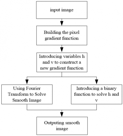
Because L0 norm is not differentiable, the global optimization problem is non-deterministic polynomial-time hard (NP-hard). Thus, variable splitting is introduced to relax the problem into two quadratic programming problems, each of which has its closed form (for the quadratic function can be derived to get its minimum). To solve the problem, alternative minimization is adopted, and two auxiliary variables h and v are introduced. Then, the final objective function can be expressed as:
$\min _{U, \mathrm{~h}, \mathrm{v}}\left\{\sum_{P}\left(U_{P}-f_{P}\right)^{2}+\lambda \cdot \mathrm{E}(\mathrm{h}, \mathrm{v})+\beta\left(\left(\partial_{x} U_{P}-\right.\right.\right.$
$\left.\left.\left.h_{P}\right)^{2}+\left(\partial_{y} U_{P}-v_{P}\right)^{2}\right)^{2}\right\}$ (4)
The complexity and noisy background of some input images hinder the subsequent detection of salient corners. Through L0 norm minimization, the low-frequency information can be filtered out, and the significant edges can be enhanced, without sacrificing image quality. As a result, the main edge information, i.e., the natural edges, of the original image is well preserved, while the background edges are largely weakened.
In formula (4), adaptive variables h and v are introduced to the energy function of gradient minimization, trying to solve the L0 norm. The two variables are obtained from the image gradient with L0 norm constraint. However, the image gradient may be wrong, owing to the noise or impurity of the image. In this case, h and v would deviate from the correct values. To solve the problem, this paper proposes an edge preserving filter to preprocess the image gradient. L1 norm is more robust than L2 for outliers. After L1 fidelity term is introduced into the model and adaptive variable w is incorporated to represent the difference between U and f, we have:
$\min _{U, \mathrm{~h}, \mathrm{v}, \mathrm{W}}\left\{\sum_{P} \alpha\left(U_{P}-f_{P}-W_{P}\right)^{2}+\left|W_{P}\right|+\lambda \cdot\right.$
$\left.\mathrm{E}(\mathrm{h}, \mathrm{v})+\beta\left(\left(\partial_{x} U_{P}-h_{P}\right)^{2}+\left(\partial_{y} U_{P}-v_{P}\right)^{2}\right)^{2}\right\}$ (5)
The adaptive variables are introduced to calculate ∇M and ∇N through alternative minimization. Formula (5) can be decomposed into three problems. Then, the alternative solutions W, (h, V) and u are searched for. The flow of the L0 gradient minimization model is shown in Figure 2.
Figure 2. Flow of the L0 gradient minimization model
3.2 Simple linear iterative clustering (SLIC)
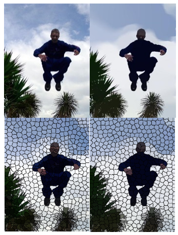
Figure 3. Image processed by L0 smoothing vs. image processed by SLIC segmentation
To detect the salient objects in the original image, SLIC [11] is adopted to segment the image into N super-pixels. This approach can divide pixels with similar features into neat and compact regions. It requires fewer parameters, runs faster, and preserves the edges better than the other super-pixel segmentation algorithms. Therefore, most super-pixel-based saliency detection algorithms use SLIC for image segmentation. After L0 smoothing, super-pixel segmentation helps to retain image edges, and ensue the uniformity of super-pixel size and distribution (Figure 3).
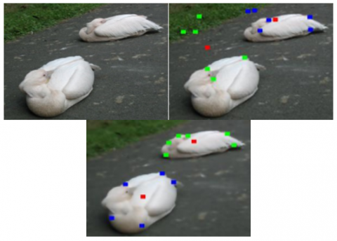
Traditional saliency detectors mostly consider image brightness, and completely ignore image colors. Hence, they are highly sensitive to the background noise of natural images. Weijer et al. [12] integrated the theory of color enhancement saliency into the Harris algorithm, yielding the Color-Harris model. The model can obtain salient corners with richer information than the brightness-based Harris corner detector.
This section employs the color-enhanced Harris algorithm to detect the corners of the salient regions in the original natural image, and eliminate the interference from near-edge salient corners. Since the image contains multiple salient objects, the salient corners are clustered on the salient regions, making it possible to preliminarily locate the salient regions. As shown in Figure 4, the salient corners generally cluster on the edges of the salient region. The number of salient objects can be calculated through automatic clustering. Note that the final saliency map is not affected by the scattered salient corners originating from background noise.
Figure 4. Color enhanced Harris corners after image smoothing
Because the image has multiple salient objects, the DBSCAN clustering algorithm [13] is introduced to cluster the salient corners. This density-based clustering algorithm assumes that the clustering effect depends on the compactness of sample distribution, for the samples in the same class are closely connected with each other. The clustering results can be obtained by dividing all closely connected samples into different classes.
The number of clusters need to be considered before detecting a single or multiple salient objects in the image. Since most background texture is filtered out by L0 gradient minimization, the corners from unsmoothed textures and tiny edges appear scattered in the image. During clustering, these corners must be differentiated from the corners of the salient objects. Therefore, the number of clusters is defined as the number of salient objects in the image.
The candidate region-based object detection algorithms assume that all objects of interest share some visual features, which make objects stand out from the background. Such an algorithm usually extracts some candidate regions from the image, i.e., the regions that may contain object(s). The candidate regions are further analyzed to detect the objects. The edge box algorithm is an excellent object detector based on candidate regions. This paper relies on the edge box algorithm [14] to position the objects in the original image.
The edge information of an object covers both color and gradient, and helps to measure the relationship between adjacent pixels accurately. With the aid of the edge information, it is possible to extract complete and significant objects, and easier to derive the saliency map from image edge intensity.
The edge box algorithm computes the score of each sliding window, according to the edge weight of the window. Firstly, the image edges are extracted by a structured edge detector, which is faster and more effective than traditional edge detectors. To count the number of edges completely contained in the sliding window, the algorithm aggregates the edges, and computes the similarity between two edges. Next, the sliding window is slid across the image, and a weight is assigned to each edge within the window. The weight reflects how much an edge is contained in the window. Finally, the weights of all edges in the window are added up, and normalized into the score of the sliding window. The score indicates the possibility that the sliding window contains objects.
5.1 Edge acquisition
The edge box algorithm relies on a structured edge detector [15] to extract the edges from the original image effectively and efficiently. Then, the peak edge value is obtained through non-maximum suppression. Any pixel whose edge modulus MP is greater than 0.1 is regarded as an edge point. However, the edge points may be misidentified or missed, if the threshold is fixed in the edge search process. To overcome the defect, the Otsu’s method can be used to adaptively calculate the segmentation threshold of edge modulus. Here, the edge moduli of image pixels are converted into gray values, forming a gray image. Then, Otsu’s image segmentation algorithm is called to optimize the segmentation threshold adaptively. Every pixel with an edge modulus larger than the adaptive threshold is defined as an edge point. The adaptive processing improves the detection accuracy of edges.
5.2 Edge grouping and similarity computing
Straight edges have a higher affinity than curved edges. Hence, the edges close to a straight line are gathered into an edge group: If the sum of the direction angle differences between every two points among eight connected edge points is greater than $\pi / 2$, these edge points are allocated to the same edge group. After obtaining multiple edge groups, the similarity between two edge groups can be calculated by:
$\mathrm{a}\left(s_{i}, s_{j}\right)=\left|\cos \left(\theta_{i}-\theta_{i j}\right) \cos \left(\theta_{j}-\theta_{i j}\right)\right|^{\gamma}$ (6)
If the mean angle between two edge groups is close to the direction of groups, there is a high affinity between the two groups.
5.3 Weights between edge groups
Each edge group is assigned a weight. The edge groups with weights of 1 are part of the inner edges of the box. The edge groups with weights of 0 are beyond or part of the outside edges of the box. The mathematical formula is as follows:
$\mathrm{w}_{b}\left(s_{i}\right)=1-\max _{T} \prod_{j}^{|T|-1} a\left(t_{j}, t_{j+1}\right)$ (7)
where, T is the series of edge group from the edge of box to $S_{i}$. Formula (7) intends to find the most similar path to derive the edges.
5.4 Score of sliding window
The edge box algorithm searches for candidate regions, using sliding windows with different positions, sizes, and aspect ratios. In the sliding search strategy, the total number of edges of the sliding window is counted according to the edge weights. After obtaining the score of each sliding window, the set of candidate regions can be obtained by ranking the regions in descending order of the score of sliding window:
$h_{b}=\frac{\sum_{i} \mathrm{w}_{b}\left(\mathrm{~s}_{i}\right) \mathrm{m}_{i}}{2\left(\mathrm{~b}_{w}+\mathrm{b}_{h}\right)^{k}}$ (8)
$m_{i}=\sum_{p \in s_{i}} m_{p}$ (9)
The flow of the edge box algorithm is summarized in Figure 5.
Figure 5. Flow of edge box algorithm
5.5 Rough positioning of salient regions
To locate the salient regions in the image, a smooth window search is performed to traverse the candidate edge boxes at different positions, scales, and aspect ratios. The traversal would produce a voting score.
Note that the translation step α, scale, and aspect ratio are fixed at 0.65. If the α value is smaller than 0.5, most of the bounding boxes contain non-salient objects. If the α value is greater than 0.8, many bounding boxes will be generated near the salient objects in the image, making the visualization confusing. After testing, the α value is set between 0.6 and 0.7, which ensures the positioning accuracy. Therefore, the α value is set to 0.65.
After smooth window search, the greedy iterative search strategy is adopted, aiming to find the largest h_b for different positions, scales, and aspect ratios. The search step is halved after each iteration. Once the translation step falls below 2 pixels, the search would be terminated.
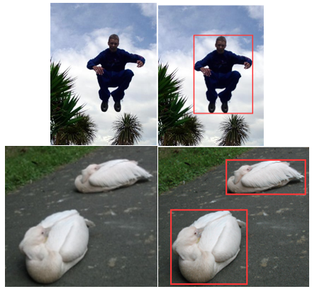
The voting score represents the possibility of a box to contain object(s). After sorting the boxes in descending order of the voting score, the number of salient objects is obtained according to the calculated number of clusters. If the number of clusters is 1, there is a salient object in the image, and the box with the highest voting score is selected for saliency detection. If the number of clusters greater than 1, there are N salient objects in the image. In this case, the top-ranking N boxes, which contain the image information, are chosen, normalized, and spliced.
In our improved edge box algorithm, the voting score of boxes containing some objects is much lower than the score of boxes containing salient objects. Thus, the boxes are sorted in descending order of the score, and the top-ranking N boxes are selected, with N equal to the number of clusters. In this way, the boxes containing the salient objects can be determined.
Figure 6 illustrates the rough positioning of salient regions.
Figure 6. Rough positioning of salient regions
The edge box algorithm resorts to structured forests [16] to find object edges. Using the BSDS 500 dataset, the image blocks and their real edge labels are taken as the training set for the random forest. Next, the principal component analysis (PCA) is performed to optimize the splitting function for each node in the forest, and adjust the number of training samples. In addition, the classification results of multiple trees are combined by an ensemble strategy. The corresponding edge labels are obtained by classifying the target image blocks with the trained random forest. Through second-order mapping, the similarity of label y is mapped to discrete label C. Finally, the edge probability map (BP) is plotted for each pixel. Based on the edge probability, super-pixels are generated, and the edge weight is recalculated to get the value of UCM.
Drawing on the super-pixel map generated previously, it is possible to construct a weighted undirected map $G=\{v, e\}$ , where each vertex $v \in V$ represents a super-pixel block $R \in \mathrm{I}$, and each edge connects two adjacent super-pixel blocks. The UCM value between $R_{u_{i}}$ and $R_{u_{j}}$ is assigned as the weight of edge $e(i, j) \in E$.
The spatial distance between pixels is measured by Euclidean distance, which reflects the consistency of the local region. But Euclidean distance may lead to misclassification based on color features. To avoid the misclassification, geodesic distance is adopted instead of Euclidean distance. The geodesic distance between two vertices $\mathrm{V}_{\mathbf{i}}$ and $\mathrm{V}_{\mathbf{j}}$ represents the cumulative weight of the shortest path on the map:
$d\left(v_{i}, v_{j}\right)=\min _{B_{1}=v_{i}, B_{2}, \ldots, B_{n}=v_{j}} \sum_{k=1}^{n-1} e\left(B_{k}, B_{k+1}\right)$ (10)
The saliency can be derived from the edge information:
$S_{E}(i, j)=\exp \left(-d^{2}\left(v_{i}, v_{j}\right) / \sigma_{1}\right)$ (11)
The Euclidean distance can be calculated by:
$d_{X Y}(\mathrm{i}, \mathrm{j})=\sqrt{\left(x_{i}-x_{j}\right)^{2}+\left(y_{i}-y_{j}\right)^{2}}$ (12)
Similarly, the standard Gaussian kernel function is used to map D﹣XY to the similarity space, producing the saliency of the spatial distance between pixels:
$\mathrm{S}_{X Y}(\mathrm{i}, \mathrm{j})=\exp \left(-d_{X Y}^{2}\left(v_{i}, v_{j}\right) / \sigma_{2}\right)$ (13)
The super-pixel on the box edges is regarded as a virtual background node. Then, a weight factor is introduced to adjust the ratio of edge information to space distance. The saliency of super-pixel P can be defined as:
$S(P)=\lambda_{1} \mathrm{~S}_{E}(P, B)+\lambda_{2} S_{X Y}(P, B)$ (14)
where, p is the super-pixel in the box; B is the virtual background node.
In general, the Bayesian model can greatly suppress the background information, without significantly inhibiting the object information. This paper treats the saliency $S(P)$ as a prior probability, and obtains the value by integrating edge information and spatial position. This computing method ensures the uniformity of the foreground, and reduces the smear effect.
The Bayesian model is a simple mathematical tool to deduce the posterior probability from the known prior probability and independent probability distribution. The independent probability distribution is usually identified through maximum likelihood estimation. This paper mainly relies on the Bayesian model proposed by Xie [17] for saliency detection, and regards saliency detection as a Bayesian reasoning problem. The posterior probability of each pixel in the image can be estimated by:
$p(s a l \mid z)=\frac{p(s a l) p(z \mid S a l)}{p(s a l) p(z \mid S a l)+(1-p(s a l)) p(z \mid b k)}$ (15)
where, $p(\operatorname{sal} \mid z)$ is the predictor of the probability for a pixel to be salient; $p(s a l)$ is the prior probability for the pixel to be salient; $1-p(s a l)$ is the prior probability for the pixel to belong to the background; $p(z \mid s a l)$ and $p(z \mid b k)$ are the observed likelihoods. The goal of this research is to estimate the probability for each pixel to be salient, and then derive the saliency map.
7.1 Calculation of prior probability
Under the current Bayesian optimization framework, some super-pixels in the foreground with similar color and background may be suppressed. Here, the prior probability is improved to generate the saliency map. Even if the color of these super-pixels is similar to that of the background, the super-pixels in the box are assigned a large weight, while the region outside the box is set to zero. If more than 80% of the pixels in a super-pixel are within the box, the super-pixel must fall in the box:
$p(s a l)=\left\{\begin{array}{lc}p_{w} \cdot S(P) & B_{i} \epsilon b o x \\ 0 & B_{i} \notin \text { box }\end{array}\right.$ (16)
where, S(P) is the saliency of the super-pixel in the box; $p_{w}=\frac{S(P)}{\sum_{p \in b o x} S(P)}$ is the mean saliency in the box.
7.2 Calculation of observation likelihood probability
The box divides the image into two parts. The region O in the box is more likely to be salient, and the region B outside the box is more likely to be the background. Then, the color histograms of O and B regions are calculated respectively. The observation likelihood probability of each pixel refers to the similarity between the pixel’s color histogram and the regional color histogram. The feature of each pixel in CIELab color can be expressed as $G(z)=\{L(z), a(z), b(z)\}$ :
$p(z \mid s a l)=\prod_{g \in\{l, a, b\}} \frac{N^{o}(g(z))}{N_{S O}}$ (17)
$p(z \mid b k)=\prod_{g \in\{l, a, b\}} \frac{N^{B}(g(z))}{N_{S B}}$ (18)
where, $N_{S O}, N_{S B}$ are the number of pixels inside and outside the box, respectively; $N^{I}(g(z))$ is the observation likelihood probability; $N^{O}(g(z))$ is the corresponding value of pixel Z of region O in the color histogram; $N^{B}(g(z))$ is the corresponding value of pixel Z of region B in the color histogram.
7.3 Calculation of the posterior probability
$p(\operatorname{sal} \mid z)=\frac{p(s a l) p(z \mid s a l)}{p(s a l) p(z \mid \operatorname{sal})+(1-p(s a l)) p(z \mid b k)}$ (19)
where, the prior probability p(sal) is the probability for a super-pixel to belong to the salient region; $1-p($ sal $)$ is the probability for the super-pixel to belong to the background.
The experiments use four datasets: MSRA10k [18], ECSSD [19], DUT-OMROM [20], and SED2 [21]. MSRA10k contains 10,000 random ground truth images of pixel level dimensions from the MSRA dataset. Compared with those of MSRA10k images, the objects and background of ECSSD images are not easily distinguishable. In DUT-OMROM, the images have relatively complex background regions, making it difficult to detect salient objects. SED2 covers 100 test images, each of which contains two objects. Despite the small scale, the objects in SED2 images are not easy to detect. The four datasets were adopted to fully demonstrate model performance in different scenarios and environments. All datasets contain manually labeled truth maps. Our model (12) was compared with 11 mainstream methods in the environment of Windows 7, Intel Core TM i7-37705 3.1 GHz CPU and 8GB RAM: (1) Itti’s model [1]; (2) spectral residual (SR) approach [22]; (3) Context-aware (CA) saliency detector [3]; (4) saliency filer (SF) [23]; (5) geodesic saliency (GS) detector [5]; (6) hierarchical saliency (HS) detector [24]; (7) graph-based manifold ranking (GMR) saliency detector [18]; (8) robust background detection (RBD) saliency optimizer [25]; (9) extended minimum barrier distance (MB+) transform [26]; (10) minimum spanning tree (MST)[27]; (11) saliency detector based on reversion correction and regularized random walk ranking (RCRR) [28].
8.1 Evaluation criteria
The detection accuracy was measured by precision, which refers to the proportion of the correctly detected objects in the entire object set of the saliency map:
Precision $=\frac{\sum S_{z} \cdot B_{z}}{\sum S_{z}}$ (20)
The detection comprehensiveness was measured by recall, which refers to the proportion of the correctly detected objects in the manually detected real objects:
Recall $=\frac{\sum S_{z} \cdot B_{z}}{\sum B_{z}}$ (21)
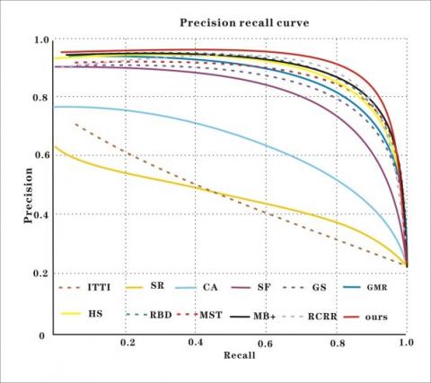
The precision and recall were measured at 256 different thresholds T = (0, 255) to reveal the robustness of each detection model. Then, a precision-recall (P-R) curve was drawn with recall as the abscissa and precision as the ordinate. The curve measures the consistency between the ground truth and the estimated saliency map. If the precision is high, then most of the detected salient regions are real salient images; if the recall is high, then the detected salient regions are complete.
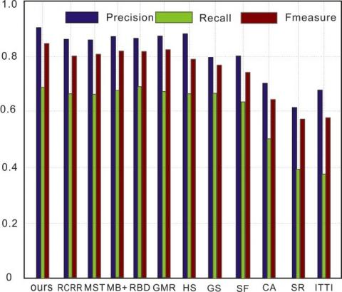
The F-measure was adopted to reflect the overall effect of precision and recall. The greater the F-measure, the better the detection effect, and the closer the estimated saliency map is to the ground truth:
$F-$ measure $=\frac{\left(1+\beta^{2}\right) \times \text { precision } \times \text { recall }}{\beta^{2} \times \text { precision }+\text { recall }}$ (22)
where, $\beta^{2}$ is usually set to 0.3.
The mean absolute error (MAE) was adopted to measure the quality of the obtained saliency map. It refers to the difference between the ground truth and the estimated saliency map:
$\mathrm{MAE}=\frac{1}{M \times N} \sum_{\mathrm{x}=1}^{M} \sum_{y=1}^{N}|S(x, y)-G T(x, y)|$ (23)
A small MEA means the estimated saliency map is close to the ground truth, and the detection model achieves a good effect.
8.2 Objective evaluation
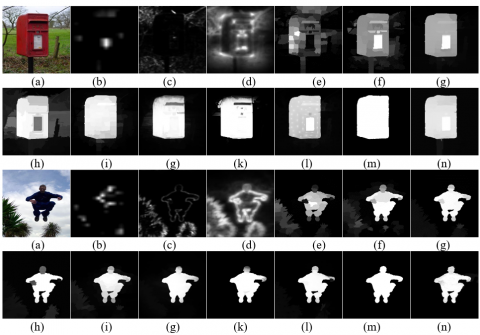
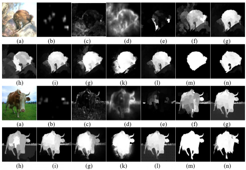
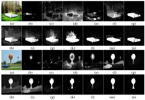
Figure 7. Detection results on MSRA10k (a) Original image (b) Itti’s model (c) SR (d) CA (e) SF (f) GS (g) HS (h) GMR (i) RBD (g) MB+ (k) MST (l) RCRR (m) Ground truth (n) Our model
Figure 8. Detection results on ECSSD (a) Original image (b) Itti’s model (c) SR (d) CA (e) SF (f) GS (g) HS (h) GMR (i) RBD (g) MB+ (k) MST (l) RCRR (m) Ground truth (n) Our model
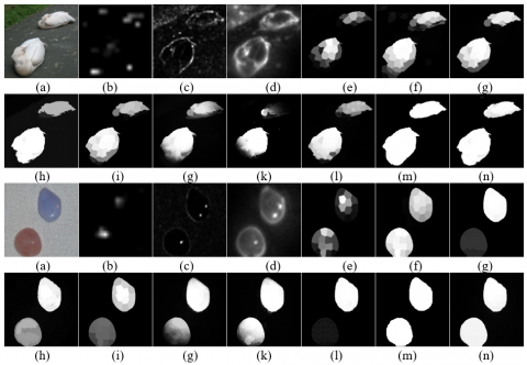
Figure 9. Detection results on DUT-OMRON (a) Original image (b) Itti’s model (c) SR (d) CA (e) SF (f) GS (g) HS (h) GMR (i) RBD (g) MB+ (k) MST (l) RCRR (m) Ground truth (n) Our model
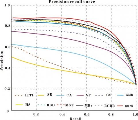
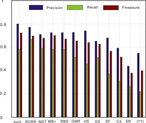
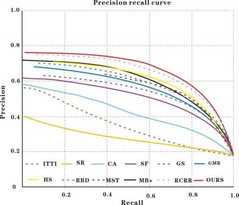
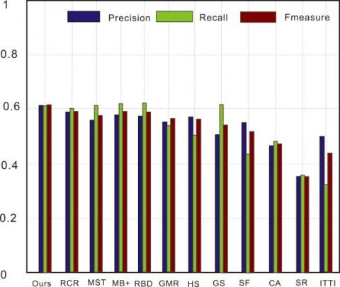
Our model considers both edge feature and spatial feature, and derives image saliency by Bayesian principle. It can effectively suppress the background, and highlight the salient objects uniformly. Our model was compared with 11 contrastive methods on each of the five experimental datasets. The results of each model on each dataset are displayed in Figures 7-10. The detection performance of all methods is presented in Figures 11-14.
On MASR10K, the saliency map derived by our model was closer to the ground truth than that derived by another method, because of the strong color difference between objects and background, and the high color consistency between them; On ECSSD and DUT-OMRON, our model achieved the best effect on background suppression and salient object highlighting, for the complexity of the background, and the small color difference between objects and background; On SED2, our model outperformed the other methods by detecting multiple salient objects, and generating a high-quality saliency map.
The superior performance of our model comes from the integration of edge boxes, edge information, and Bayesian theory into the optimization process of saliency detection. That is how our model can detect objects accurately, suppress the background information, and ensure the uniformity of salient regions.
Figure 10. Detection results on SED2 (a) Original image (b) Itti’s model (c) SR (d) CA (e) SF (f) GS (g) HS (h) GMR (i) RBD (g) MB+ (k) MST (l) RCRR (m) Ground truth (n) Our model
(a)
(b)
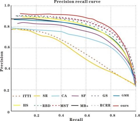
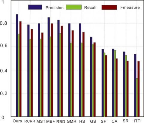
Figure 11. Detection performance on MSRA10k (a) P-R curve; (b) Precision, recall, and F-measure at different thresholds
(a)
(b)
Figure 12. Detection performance on ECSSD (a) P-R curve; (b) Precision, recall, and F-measure at different thresholds
(a)
(b)
Figure 13. Detection performance on DUT-OMRON (a) P-R curve; (b) Precision, recall, and F-measure at different thresholds
(a)
(b)
Figure 14. Detection performance on SED2 (a) P-R curve; (b) Precision, recall, and F-measure at different thresholds
Table 1. MAEs of different methods
|
Dataset |
Itti’s model |
SR |
CA |
SF |
GS |
GMR |
RBD |
HS |
MB+ |
MST |
RCRR |
Our model |
|
|
MSRA10k |
MAE |
0.212 |
0.231 |
0.236 |
0.174 |
0.143 |
0.113 |
0.107 |
0.148 |
0.13 |
0.121 |
0.116 |
0.105 |
|
ECSSD |
MAE |
0.274 |
0.265 |
0.311 |
0.231 |
0.216 |
0.184 |
0.174 |
0.229 |
0.193 |
0.172 |
0.221 |
0.158 |
|
DUT-OMRON |
MAE |
0.198 |
0.181 |
0.254 |
0.183 |
0.18 |
0.152 |
0.144 |
0.227 |
0.192 |
0.167 |
0.172 |
0.132 |
|
SED2 |
MAE |
0.245 |
0.212 |
0.222 |
0.182 |
0.124 |
0.131 |
0.128 |
0.165 |
0.117 |
0.112 |
0.149 |
0.109 |
As shown in Figures 11-14, the P-R curve of our model was higher than that of any other method. That is, the detection results of our model were closer to the ground truth than those of the other methods. Taking ECSSD for example, the recall of our model was low in the range of [0.9, 1], due to the impact of threshold on detection accuracy. With the decrease of recall and growth of threshold, the detection precision of most methods was on the rise. Our model achieved the fastest rise of the precision. After the recall fell below 0.6, our model reached the peak precision. In addition, our model realized the greatest F-measure among all methods. Although some methods achieved comparable precision and recall, our model boasted the best overall detection performance on all four datasets.
Table 1 shows the MAEs of the 12 methods on the four datasets. The best results are marked in red. It can be observed that our model achieved the lowest MAEs on all four datasets. The results show that our model outshined the other methods on every dataset.
Our model was further contrasted with the cascaded partial decoder (CPD) [17], a deep learning tool, on ECSSD and SED2. The results in Table 2 show that the recall of CPD was higher than that of our model, while the F-measure and precision of CPD were lower than those of our model. Overall, the metrics of our model were relatively close to the saliency detection results of deep learning, indicating the effectiveness of our model in saliency detection.
In addition, the mean running time of our model was compared with that of SR, FT, RC, GS, and GMBR. This is to measure the complexity of different methods. The results in Table 3 suggest that the frequency domain-based FT had a shorter running time than our model. However, this frequency domain algorithm cannot retain enough high-frequency information, or obtain salient regions with clear edges. Besides, our algorithm consumed a shorter running time than GS and GBMR, and better performance metrics than them. In general, our model had obvious advantages over the contrastive methods, whether by visual saliency results or performance metrics. Hence, our model is an effective saliency detector. The time efficiency of our model is attributable to the following facts:
The model involves two phases: positioning salient objects in the original image; computing the object position within selected salient regions. In each selected region, the calculation process is not much interfered by the background. Besides, our model reduces the computational area, while the other methods take all image pixels as one calculation unit.
Table 2. Effectiveness of our model vs. that of CPD
|
Metrics |
Precision |
Recall |
F-Measure |
|||
|
Datasets |
ECSSD |
SED2 |
ECSSD |
SED2 |
ECSSD |
SED2 |
|
Our model |
0.7637 |
0.6971 |
0.6618 |
0.4975 |
0.7394 |
0.6213 |
|
CPD |
0.7136 |
0.8635 |
0.6835 |
0.6482 |
0.6965 |
0.8017 |
Table 3. Mean running time of different methods
|
Methods |
Our method |
SR |
FT |
RC |
GS |
GBMR |
|
Mean running time (s) |
1.265 |
0.249 |
0.967 |
0.186 |
3.438 |
1.577 |
This paper relies on the clustering algorithm to get the number of image corners, and employs the edge box algorithm to select the candidate regions of salient objects. According to the number of clusters, single- and multi-object saliency of the original image are handled separately. The saliency computed by geodesic distance was taken as a prior probability, while the color distribution of the inner and outer regions of the bounding box was adopted as the observation likelihood probability. Finally, a clear and smooth saliency map was obtained by the Bayesian formula. The effectiveness of the proposed saliency detection model was confirmed by the expeirmental results on four benchmark datasets. Comparative analysis shows that our model is superior to the existing salient object detection methods, as evidenced by multiple metrics. Our model has a significant advantage over images strong edge information and multiple salient objects. In future, our model will be applied to dynamic videos, and three-dimensional (3D) images.
[1] Itti, L., Koch, C., Niebur, E. (1998). A model of saliency-based visual attention for rapid scene analysis. IEEE Transactions on Pattern Analysis and Machine Intelligence, 20(11): 1254-1259. https://doi.org/10.1109/34.730558
[2] Hou, X., Harel, J., Koch, C. (2011). Image signature: Highlighting sparse salient regions. IEEE Transactions on Pattern Analysis and Machine Intelligence, 34(1): 194-201. https://doi.org/10.1109/TPAMI.2011.146
[3] Goferman, S., Zelnik-Manor, L., Tal, A. (2011). Context-aware saliency detection. IEEE Transactions on Pattern Analysis and Machine Intelligence, 34(10): 1915-1926. https://doi.org/10.1109/TPAMI.2011.272
[4] Zhu, W., Liang, S., Wei, Y., Sun, J. (2014). Saliency optimization from robust background detection. In Proceedings of the IEEE Conference on Computer Vision and Pattern Recognition, pp. 2814-2821.
[5] Wei, Y., Wen, F., Zhu, W., Sun, J. (2012). Geodesic saliency using background priors. In European Conference on Computer Vision, pp. 29-42. https://doi.org/10.1007/978-3-642-33712-3_3
[6] Cheng, M.M., Mitra, N.J., Huang, X., Torr, P.H., Hu, S.M. (2014). Global contrast based salient region detection. IEEE Transactions on Pattern Analysis and Machine Intelligence, 37(3): 569-582. https://doi.org/10.1109/TPAMI.2014.2345401
[7] Zeng, Y., Feng, M., Lu, H., Yang, G., Borji, A. (2018). An unsupervised game-theoretic approach to saliency detection. IEEE Transactions on Image Processing, 27(9): 4545-4554. https://doi.org/10.1109/TIP.2018.2838761
[8] Zhang, P., Wang, D., Lu, H., Wang, H., Yin, B. (2017). Learning uncertain convolutional features for accurate saliency detection. In Proceedings of the IEEE International Conference on Computer Vision, pp. 212-221.
[9] Liu, N., Han, J. (2018). A deep spatial contextual long-term recurrent convolutional network for saliency detection. IEEE Transactions on Image Processing, 27(7): 3264-3274. https://doi.org/10.1109/TIP.2018.2817047
[10] Xu, L., Lu, C., Yi, X. (2011) Image smoothing via l0gradient minimization. ACM Transactions on Graphics, 30(6):1-12.
[11] Achanta, R., Shaji, A., Smith, K., Lucchi, A., Fua, P., Süsstrunk, S. (2012). SLIC superpixels compared to state-of-the-art superpixel methods. IEEE Transactions on Pattern Analysis and Machine Intelligence, 34(11): 2274-2282. https://doi.org/10.1109/TPAMI.2012.120
[12] Van de Weijer, J., Gevers, T., Bagdanov, A.D. (2005). Boosting color saliency in image feature detection. IEEE Transactions on Pattern Analysis and Machine Intelligence, 28(1): 150-156. https://doi.org/10.1109/TPAMI.2006.3
[13] Ester, M., Kriegel, H.P., Sander, J., Xu, X. (1996). A density-based algorithm for discovering clusters in large spatial databases with noise. In Kdd, 96(34): 226-231.
[14] Zitnick, C.L., Dollár, P. (2014). Edge boxes: Locating object proposals from edges. In European Conference on Computer Vision, pp. 391-405. https://doi.org/10.1007/978-3-319-10602-1_26
[15] Arbeláez, P., Pont-Tuset, J., Barron, J.T., Marques, F., Malik, J. (2014). Multiscale combinatorial grouping. In Proceedings of the IEEE Conference on Computer Vision and Pattern Recognition, pp. 328-335.
[16] Dollár, P., Zitnick, C.L. (2013). Structured forests for fast edge detection. In Proceedings of the IEEE International Conference on Computer Vision, pp. 1841-1848.
[17] Xie, Y., Lu, H. (2011). Visual saliency detection based on Bayesian model. In 2011 18th IEEE International Conference on Image Processing, pp. 645-648. https://doi.org/10.1109/ICIP.2011.6116634
[18] Yang, C., Zhang, L., Lu, H., Ruan, X., Yang, M.H. (2013). Saliency detection via graph-based manifold ranking. In Proceedings of the IEEE Conference on Computer Vision and Pattern Recognition, pp. 3166-3173.
[19] Yan, Q., Xu, L., Shi, J., Jia, J. (2013). Hierarchical saliency detection. In Proceedings of the IEEE Conference on Computer Vision and Pattern Recognition, pp. 1155-1162.
[20] Huang, L., Pashler, H. (2007). Working memory and the guidance of visual attention: Consonance-driven orienting. Psychonomic Bulletin & Review, 14(1): 148-153. https://doi.org/10.3758/BF03194042
[21] Wang, Y., Yang, J., Yin, W., Zhang, Y. (2008). A new alternating minimization algorithm for total variation image reconstruction. SIAM Journal on Imaging Sciences, 1(3): 248-272. https://doi.org/10.1137/080724265
[22] Hou, X., Zhang, L. (2007). Saliency detection: A spectral residual approach. In 2007 IEEE Conference on Computer Vision and Pattern Recognition, pp. 1-8. https://doi.org/10.1109/CVPR.2007.383267
[23] Perazzi, F., Krähenbühl, P., Pritch, Y., Hornung, A. (2012). Saliency filters: Contrast based filtering for salient region detection. In 2012 IEEE Conference on Computer Vision and Pattern Recognition, pp. 733-740. https://doi.org/10.1109/CVPR.2012.6247743
[24] Yan, Q., Xu, L., Shi, J., Jia, J. (2013). Hierarchical saliency detection. In Proceedings of the IEEE Conference on Computer Vision and Pattern Recognition, pp. 1155-1162.
[25] Zhu, W., Liang, S., Wei, Y., Sun, J. (2014). Saliency optimization from robust background detection. In Proceedings of the IEEE Conference on Computer Vision and Pattern Recognition, pp. 2814-2821.
[26] Zhang, J., Sclaroff, S., Lin, Z., Shen, X., Price, B., Mech, R. (2015). Minimum barrier salient object detection at 80 fps. In Proceedings of the IEEE International Conference on Computer Vision, pp. 1404-1412.
[27] Tu, W.C., He, S., Yang, Q., Chien, S.Y. (2016). Real-time salient object detection with a minimum spanning tree. In Proceedings of the IEEE Conference on Computer Vision and Pattern Recognition, pp. 2334-2342.
[28] Yuan, Y., Li, C., Kim, J., Cai, W., Feng, D.D. (2017). Reversion correction and regularized random walk ranking for saliency detection. IEEE Transactions on Image Processing, 27(3): 1311-1322. https://doi.org/10.1109/TIP.2017.2762422