Qiuhe Huang
© 2021 IIETA. This article is published by IIETA and is licensed under the CC BY 4.0 license (http://creativecommons.org/licenses/by/4.0/).
OPEN ACCESS
The traditional image sharpness enhancement algorithm faces several defects, namely, the lack of details, and the poor subjective effect. To solve these defects, this paper proposes an image sharpness enhancement algorithm based on the Green function. Specifically, the Retinex model was employed to ensure that the enhanced image has outstanding details, and the Poisson’s equation was solved to maintain the consistency between the enhanced image and the original image in the gradient domain. Then, adaptive brightness mapping was carried out to determine the boundary conditions suitable for display, and the boundary of the region was sampled to reduce the complexity of our algorithm. Experimental results show that our algorithm improved the contrast and sharpness of images from the levels of contrastive image enhancement algorithms.
image enhancement, green function, Poisson equation, gradient domain
With the in-depth study of image processing technology, digital images are widely used in more and more fields [1, 2]. The common defects of these images, such as low quality and poor subjective effect, greatly restrict the effect of subsequent image processing. To extract as much key information from the low-quality images as possible, image processing techniques like image enhancement have been proposed to process such images.
As a computer vision technique, image enhancement has several advantages in processing digital images. For example, the visual experience can be improved to meet the needs of visual appreciation; the image details can be reproduced to enhance the detection and recognition ability in the field of computer vision. The enhancement of image quality, especially the sharpness of low-illumination images, is a key measure for information reproduction, and a research hotspot in image processing.
Low-illumination images are complex and diverse. For an image with low global brightness, the enhancement aims to elevate the brightness and contrast of the image, and suppress noise amplification. However, most low-illumination images face low local brightness, local brightness saturation, or even overexposure. To enhance such images, consideration should be given to multiple issues: improving the brightness of dark areas, preventing the loss of details in bright areas, and even compressing the brightness of overexposed areas to highlight the details.
For these considerations, great efforts have been paid to improve image enhancement technology. A good image enhancement algorithm should be able to highlight the local or global features of the original image, and improve the quality and visual effect of the image.
2.1 Image enhancement
Many image enhancement algorithms can improve the subjective visual effect of the original image to a certain extent. But each algorithm has its own defects. For instance, histogram equalization [3] can greatly enhance the global contrast of the image, but at the expense of the contrast in local areas. Through histogram equalization, the gray values are easily combined excessively, resulting in the loss of some details of the original image. As a result, the enhanced image has a reduced quality. With the aid of histogram segmentation, Cao et al. [4] performed histogram equalization of each sub histogram to improve the brightness of low-illumination images; the histogram segmentation alleviates the problem of excessive enhancement to a certain extent. Qadar et al. [5] proposed a recursive separation weighted histogram equalization algorithm, which decomposes the histogram into several sub histograms, weighs each sub histogram, and then implement histogram equalization; however, the quality of the enhanced image often degrades, due to the loss of statistical information.
Some researchers held that the spatial information of the image is more suitable for image enhancement than the first-order statistics. For example, Zhou et al. [6] put forward the context and variation contrast enhancement algorithm, which adjusts the image with two-dimensional (2D) histogram. Under the best contrast tone mapping framework, Song et al. [7] proposed a new image enhancement algorithm that overcomes the limitations of contrast enhancement histogram, using the joint probability of spatial information.
2.2 Retinex model
The Retinex model [8], a popular model in the field of image enhancement, mimics human’s visual perception of brightness and colors. The model is built on the constancy of colors: Under the irradiation of natural light, different objects reflect lights of different wavelengths to human eyes, creating different colors; in other words, the colors are not intrinsic properties of the objects.
Currently, there are four types of Retinex models: path model [9], partial differential equation model [10], center surround model [11] and variational model [12]. The random spray Retinex model proposed by Provenzi et al. [13] has too many parameters and a huge computing load. The primary defect of the path model is that the conditions of local information processing no longer apply, when the path increases and the scope expands. Wu and Wu [14] analyzed Retinex model from a new perspective, and constructed a partial differential equation model. The model can achieve accurate results with only a few parameters. Xie et al. [15] proposed single scale Retinex (SSR) algorithm and multi-scale Retinex (MSR) algorithm, but the two algorithms have problems like unnatural color. Ma et al. [16] designed a multi-scale Retinex algorithm with color restoration ability, and corrected the enhanced image with the color recovery factor. Fine and MacLeod [17] presented a natural reservation algorithm based on prior brightness statistics, and obtained satisfactory results of quality enhancement. The variational model is based on prior construction constraints. Hou et al. [18] developed a Retinex algorithm under the variational framework, under the assumption that the illumination components vary smoothly in space, and calculated the illumination by gradient descent. Xie et al. [19] proposed a method to estimate the probability of illumination and reflection at the same time, and demonstrated its good results on detail enhancement. Li and Yin [20] evaluated the enhanced image by adding a coefficient matrix. This evaluation method does well in image enhancement, but the enhanced image is often noisy owing to the excessive brightness enhancement.
The above analysis shows that the Retinex model has a serious halo phenomenon in the enhanced image, despite adopting a hierarchical structure. The halo covers the edge details of the high-contrast image. The contrast can be obviously enhanced through nonlinear grayscale stretching. Nevertheless, this approach fails to consider the subjective visual effect of human eyes, and underestimates the image information entropy through the combination of gray values, leading to a poor visual effect of the enhanced image.
2.3 Thesis statement
To solve the defects of existing algorithms, this paper presents an image sharpness enhancement algorithm based on the Green function is proposed. To retain as much image details as possible, the illumination layer separated by Retinex model was enhanced separately without changing the detail layer. The former layer contains the details of the original image, while the latter covers the contrast information of the image.
The Retinex theory is unfolded around three hypotheses: (1) The colors perceived by human eyes are not the intrinsic properties of the object, but the product of the interaction between light and the object. (2) Each color region is made up of three primary colors (red, green, and blue) with fixed wavelength; different colors of objects are formed through the light reflected by the objects, which vary in the reflectance to light of different wavelengths. (3) The three primary colors determine the color of each unit, and different colors are composed of different combinations of the three primary colors.
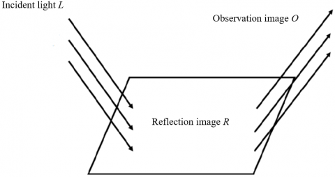
According to the Retinex theory, the essential properties of an object hinge on the object’s ability to reflect light of different wavelengths. The color of the object remains constant, and has nothing to do with illumination. However, the object color perceived by human eyes could change, when the object is under ifferent illumination conditions. Mimicking the imaging process of human eyes, the Retinex theory can be described as shown in Figure 1.
Figure 1. Retinex theory diagram
The object is irradiated by the incident light. The light reflected by the object than enters the human eyes. The planar image thus forms is the image observed by human eyes, while the image reflecting the intrinsic properties of the object is called the reflection image. Then, the observation image O with a known number of pixels can be expressed as the product of the incident light L and the reflection image R.
$O=L \times R$ (1)
The intensity of the incident light determines the brightness of the object.
The traditional Retinex algorithm transforms the operation into the logarithmic domain:
$o=\log (O)$ (2)
$l=\log (L)$ (3)
$r=\log (R)$ (4)
According to formula (1), the logarithmic field can be defined as:
$o=\log (0)=\log (L \times R)$$=\log (L)+\operatorname{lo} g(R)=r+l$ (5)
Formula (5) transforms multiplication operation into addition operation. The logarithmic domain method both suits the human visual system, and reduce the amount of calculation.
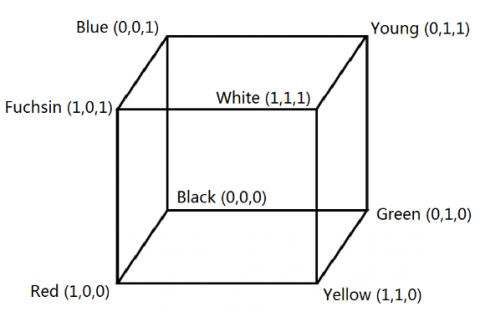
The processing of digital color images is essentially the adjustment of the pixels of the three channels: red (R), green (G), and blue (B). In the classic Retinex algorithms, the Retinex model is adopted to adjust the brightness of each channel. However, the processed color image often faces color distortion, because the brightness is adjusted by different magnitudes in different channels. To make the low-illumination image brighter, the processed image should be converted to a color model with brightness channel, and only the brightness channel should be processed.
The RGB is the most widely used color space in computer applications. The RGB color space is the three-dimensional (3D) space formed by all possible combinations of the three primary colors (Figure 2).
Figure 2. RGB color space model
The SSR is the most classic RGB-based Retinex algorithm. The algorithm takes Gaussian function as the center surround function, and the Gaussian smoothing result of the original image as illumination. The Gaussian surround function can be defined as:
$G(x, y)=\vartheta e^{-\left(x^{2}+y^{2}\right) / \sigma^{2}}$ (6)
where, σ is the scale parameter; ϑ is the normalization factor, whose value satisfies the following integral function:
$\iint G(x, y) d x d y=1$ (7)
To ensure the high similarity between the enhanced image and the original image, it is necessary to transform solving pixel brightness in each bright region into solving the corresponding Poisson equation, without changing the information in the gradient domain. This is because some information of the original image belongs to the gradient domain.
The Poisson equation based on gradient domain adheres to the following principle:
Let F be the gradient image. According to the properties of the gradient operator ∇, the illumination layers I and F satisfy the following relationship:
$F(x, y)=\nabla I(x, y)$ (8)
According to the consistency of gradient, the enhanced illumination layer $\tilde{I}$ can be expressed as:
$F(x, y)=\nabla \tilde{I}(x, y)$ (9)
For one-dimensional (1D) data, $\tilde{I}$ can be obtained by directly integrating both sides of formula (9); for 2D data, the enhanced image cannot be directly integrated, for formula (9) has no solution. Then, the solution of formula (9) can be indirectly obtained by:
$\min _{I} \iint\|\nabla \tilde{I}(x, y)-F(x, y)\|^{2} d x d y$ (10)
$P(x, y)=\|\nabla \tilde{I}(x, y)-F(x, y)\|^{2}$ (11)
According to the principle of variational method, formula (10) satisfies the Euler-Lagrange equation.
$\frac{\partial P}{\partial \tilde{I}}-\frac{d}{d x} \frac{\partial P}{\partial \tilde{I}_{x}}-\frac{d}{d x} \frac{\partial P}{\partial \tilde{I}_{y}}=0$ (12)
Substituting P into formula (12), the Poisson equation can be established as:
$\Delta \tilde{I}(x, y)=\operatorname{divF}(x, y)$ (13)
where, ∆ is the Laplacian operator; div is the divergence operator. Then, the following relationship is satisfied:
$\left\{\begin{array}{l}\Delta \tilde{I}(x, y)=\frac{\partial^{2} \tilde{I}(x, y)}{\partial x}+\frac{\partial^{2} \tilde{I}(x, y)}{\partial y} \\ \operatorname{divF}(x, y)=F_{x}(x, y)+F_{y}(x, y)\end{array}\right.$ (14)
The existence of halo is a sign of the serious gray mutation near the edge of the illumination image, for the algorithm emphasizes the spatial relationship over the gray relation between pixels. The halo can be effectively suppressed through bilateral filtering, which synthesizes the gray value change of pixels based on their relative positions.
The only difference between bilateral filtering and the SSR algorithm lies in the selection of convolution kernel. The convolution kernel of bilateral filtering can be defined as:
$\begin{aligned} L_{x, y}(i, j) &=\gamma \exp \left[-\frac{(i-x)^{2}+(j-x)^{2}}{2 \sigma_{s}^{2}}\right.\\ & \left.-\frac{[S(i, j)-S(x, y)]^{2}}{2 \sigma_{r}^{2}}\right] \end{aligned}$ (15)
where, $\sigma_{S}^{2}$ and $\sigma_{r}^{2}$ are empty value and gray value, respectively.
The shape of the bilateral filter depends on the gray value and position of pixels. Therefore, the time complexity of bilateral filtering is O(r2), far greater than the O(r) of the SSR.
To keep the enhanced image consistent with the original image in the gradient domain, image enhancement was transformed into solving the Poisson equation as shown in formula (13).
When the gradient image of the illumination layer of the original image is known, the enhanced image $\tilde{I}$ can be obtained, after the Poisson equation of formula (13) has been solved. Next, $\tilde{I}$ should be replaced by the original illumination image I of formula (1), in order to produce the enhanced image with preserved details.
4.1 Solving Poisson equation with Green function
The Poisson equation can be solved by many methods, such as the Green function, fast Fourier transform, central difference method, and multigrid method [21]. In this paper, the second Green function method, which is based on Dirichlet boundary condition, is adopted to solve the Poisson equation of formula (13). The Dirichlet boundary condition controls the brightness of the entire planar region. That is, the enhanced image can be obtained by the Green function, as long as the boundary pixel brightness in the region with low brightness or high exposure are mapped to the brightness suitable for human eyes.
Let ϵ denote a planar closed region with σϵ as the boundary, ϵ* denote the boundary condition, and r denote any point in ϵ. Then, formula (14) satisfies the Dirichlet boundary condition:
$\left\{\begin{array}{c}\Delta \tilde{I}(r)=\operatorname{div} \nabla F(r) \\ \left.\tilde{I}(r)\right|_{\sigma \epsilon}=\tilde{I}^{*}(r)\end{array}\right.$ (16)
According to the second Green function, the solution of formula (16) can be expressed as:
$\tilde{I}(r)=-\int_{\sigma \epsilon} \tilde{I}^{*}\left(r_{0}\right) \frac{\partial G\left(r, r_{0}\right)}{\partial n_{0}} d s$
$-\iint_{\epsilon} \operatorname{div} \nabla F(r) \times G\left(r, r_{0}\right) d \sigma$ (17)
where, n0 is the outer normal direction of σϵ; r0 is the position of point source charge in the planar region ϵ; G(r,r0) is the guarantee that the Green function satisfies the point source function and the boundary homogeneity:
$\left\{\begin{array}{c}\left.G\left(r, r_{0}\right)\right|_{\sigma \epsilon}=0 \\ \Delta G\left(r, r_{0}\right)=-\vartheta\left(r-r_{0}\right)\end{array}\right.$ (18)
where, $\tilde{I}^{*}\left(r_{0}\right)$ and div∇F(r) are known; the Green function G is the only unknown. Formula (13) can be solved if the Green function satisfies the point source function and the boundary homogeneity.
The Green function is usually constructed by the electric image method, which can provide the Green function of a regular and symmetrical region. For a planar circular region ϵ, it is assumed that the dielectric constant ε equals 1, a standard punctual charge with q is placed at any point in ϵ, and the boundary is composed of m non-repeated points that satisfies σϵ∈{b1,b2,…,bm}, ∀bi∈R2. By the principle of the electric image method, the equivalent charge q' of the induced charge formed by the point charge at any boundary point falls on the extension line between the center of the circle and point q, and lies outside the circle.
Figure 3. Diagram of point charge, boundary point, and equivalent charge
The point charge, boundary point, and equivalent charge is shown in Figure 3, where c is the center of the circle, r0 is the point charge, r1 is the equivalent charge, and bi is any boundary point. These parameters satisfy the following relationship:
$\frac{\left\|c-b_{i}\right\|}{\left\|c-r_{1}\right\|}=\frac{\left\|c-r_{0}\right\|}{\left\|c-b_{i}\right\|}$ (19)
Since ∠r0cbi=∠bicr1, we have ∆r0cbi=∆bicr1. Then, the following relationship can be derived:
$\frac{\left\|b_{i}-p\right\|}{\left\|x_{n}-b_{i}\right\|}=\frac{R}{\left\|c-x_{0}\right\|}$ (20)
According to the theory of electromagnetic field, the Green function describes the potential of point charge r0 in r. For any point in unbounded space, the Green function can be expressed as:
$G\left(r, r_{0}\right)=\frac{q}{2 \pi} \cdot \frac{1}{\ln \left\|r-r_{0}\right\|}$ (21)
For the circular region in Figure 3, the potential of point r is the superposition of the potential generated by r0 in the unbounded space and the potential generated by the equivalent charge of the boundary. Thus, G(r,r0) can be defined as:
$G\left(r, r_{0}\right)=\frac{q}{2 \pi} \cdot \frac{1}{\ln \left\|r-r_{0}\right\|}+\frac{q^{\prime}}{2 \pi} \cdot \frac{1}{\ln \left\|r-r_{1}\right\|}$ (22)
Because the Green function satisfies boundary homogeneity, that is, the potential at any boundary point bi equals zero, the Green function of any boundary bi must be equal to zero. Thus, we have:
$G\left(b_{i}, r_{0}\right)=\frac{q}{2 \pi} \cdot \frac{1}{\ln \left\|b_{i}-r_{0}\right\|}+\frac{q^{\prime}}{2 \pi} \cdot \frac{1}{\ln \left\|b_{i}-r_{1}\right\|}$ (23)
Sorting out formulas (19) and (20), and substituting the result into formula (23):
$q^{\prime}=-q \frac{\ln R}{\ln \left\|c-r_{\Omega}\right\|}$ (24)
Substituting formula (24 into formula (22), the Green function in circular region can be expressed as:
$G\left(r, r_{0}\right)=\frac{q}{2 \pi} \cdot \frac{1}{\ln \left\|r-r_{0}\right\|}$
$-\frac{q \ln R}{2 \pi \ln \left\|c-r_{0}\right\| l n\left\|r-r_{1}\right\|}$ (25)
Substituting formula (25) into formula (17), the solution of Poisson equation, i.e., the enhanced image, can be obtained.
According to formula (17), solving the gray value of pixels in the region is equivalent to solving the second type curve integral of the Green function for the boundary of the whole region. The complexity of the algorithm is O(mn), with m being the number of boundary points, and n being the total number of pixels in the region. The high complexity is not conducive to real-time processing. Thus, it is necessary to reduce the complexity of the algorithm by the boundary sampling with equal interval.
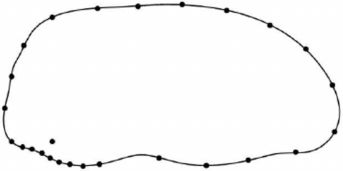
The boundary sampling with equal interval can be implemented by the following principle: First, the set of boundary points can be expressed as $\sigma \tilde{\epsilon}=\left\{\tilde{b}_{1}, \tilde{b}_{2}, \ldots, \tilde{b}_{s}\right\}$ based on the boundary points sampled with equal interval $\sigma \in$. After sampling, the Euclidean distance from any point xi in the region to the boundary point $\tilde{b}_{j}$ after sampling is $\left\|x_{i}-\tilde{b}_{j}\right\|$. As can be seen from formula (17), when the point charge is close to the boundary point, the boundary point contributes greatly to the curve integral. The inverse is also true. Hence, a threshold Tτ can be set to measure the distance. The threshold must satisfy:
$\left\|x_{i}-\tilde{b}_{j}\right\|<T_{\tau}$ (26)
Figure 4 shows a set of points sampled from a point charge at any position in the region and the corresponding boundary. It can be seen that the effectiveness of the boundary points being sampled increases with the proximity to the point. This means, when formula (26) is satisfied, the number of boundary pixels is reduced to lower the complexity of the algorithm.
Figure 4. Boundary sampling diagram
4.2 Adaptive brightness mapping
Formula (17) suggests that it is possible to obtain the gray values of the pixels in the planar region, after the determination of the Dirichlet boundary condition of the region acted by Green function. Thus, the global brightness of the pixels in the planar region is controlled by the gray values of the boundary pixels.
The human eyes have different sensitivities to different brightness. For example, with the decrease of brightness, the local contrast is reduced, and the human eyes are less able to distinguish between details. Then, the image quality will be rather poor. The strong light, which greatly stimulates the human eyes, would submerge the image details.
If the planar region is dark, the boundary pixels should be made brighter; if the planar region is bright, the boundary pixels should be made darker. Then, the boundary conditions need to be brought into the Green function to solve the Poisson equation, and thus improve the visual effect of the human eyes.
Table 1. Piecewise adaptive brightness mapping
|
Brightness of illumination image |
Piecewise adaptive brightness |
|
$\widehat{K} \leq-3.93$ |
-2.87 |
|
$-3.93<\widehat{K} \leq-1.43$ |
$(0.403 \widehat{K}+1.57)^{2.17}-2.87$ |
|
$-1.43<\widehat{K} \leq 0$ |
$\widehat{K}-0.393$ |
|
$0<\widehat{K} \leq 1.88$ |
$(0.246 \widehat{K}+0.66)^{2.72}-0.72$ |
|
$\widehat{K}>1.88$ |
$\widehat{K}-1.257$ |
Note: $\widehat{K}$ represents brightness (unit: cd/m2).
This paper chooses the piecewise adaptive brightness mapping to map the brightness of boundary pixels to the level suitable for the human eyes. Table 1 shows the procedure of this mapping strategy.
In the gray image, the gray value measures the brightness of the corresponding pixel. Therefore, the piecewise adaptive brightness mapping cannot be directly applied. Instead, the gray value should be firstly converted into the corresponding brightness. Let Kmin and Kmax be the minimum and maximum brightness values of the display, respectively. Suppose the gray values of pixels change between 0 and 255. Then, the gray value of a pixel can be converted into brightness by:
$K(x, y)=I(x, y) / 255 \times\left(K_{\max }-K_{\min }\right)$ (27)
where, I is the illumination image obtained by fast bilateral filtering; K is the corresponding brightness image. Then, the brightness image needs to be brought into Table 1 to get the adaptive brightness of each pixel. Finally, the brightness should be converted into gray value by formula (26), thereby producing the corresponding gray image.
To sum up, the proposed image sharpness enhancement algorithm is implemented in the following procedure: Firstly, the original image is divided into a group of symmetrical closed planar regions. Next, the Poisson equation is solved according to the Dirichlet boundary condition of the region. Since the electric image method only applies to regular and symmetrical regions, the image is divided into several regular circular sub blocks through secondary partition. The solution of Poisson equation corresponding to each sub block is obtained by the electric image method. Finally, the solutions of all sub blocks are stitched into the enhanced image. The specific steps of the algorithm are as follows:
Step 1. Separate the illumination layer from the detail layer by fast bilateral filtering.
Step 2. Divide the illumination image into several tangent circular regions, according to the size of the original image.
Step 3. Segment the brightness of all boundary points to obtain the first boundary conditions of all regions.
Step 4. Extract a region, and place a point charge q at any point in that region. Apply the boundary sampling algorithm with interval d to the region, and solve the Green function of the region.
Step 5. Substitute the Green function into formula (17) to calculate the gray value of each pixel in the region, and mark the pixel that has been solved.
Step 6. Repeat Steps 4-5 until all partially cut circular regions have been traversed.
Step 7. Divide the remaining pixels into sub blocks by secondary partition.
Step 8. Place a point charge at any point in the unlabeled pixels of a region being divided into sub blocks, perform the boundary sampling algorithm with interval d on the region, and solve the Green function of the region.
Step 9. Substituting the Green function into formula (17) to calculate the gray value of each unlabeled pixel.
Step 10. Repeat Steps 8-9 until all the sub blocks have been traversed.
Step 11. Bring the enhanced image into Retinex model to get the enhanced image.
Under the condition of no reference image, the image clarity measuring method [22] can achieve high accuracy, monotony, and consistency. Therefore, this method was adopted to evaluate the quality of the image enhanced by various algorithms.
Our experiments use two of the most commonly used classic images, namely, cameraman and Lena. The performances of all image sharpness enhancement algorithms on cameraman and Lena are listed in Tables 2 and 3, respectively.
Table 2. Performance of all algorithms on cameraman
|
Algorithm |
Information entropy |
Image definition |
Standard deviation |
|
Original image |
7.03 |
4.28 |
62.36 |
|
Equalization algorithm |
6.83 |
4.33 |
72.68 |
|
SSR algorithm |
7.21 |
6.85 |
66.41 |
|
Nonlinear expansion algorithm |
7.13 |
5.91 |
62.41 |
|
Our algorithm |
7.75 |
7.79 |
82.53 |
Table 3. Performance of all algorithms on Lena
|
Algorithm |
Information entropy |
Image definition |
Standard deviation |
|
Original image |
7.46 |
4.89 |
47.86 |
|
Equalization algorithm |
7.12 |
3.75 |
58.61 |
|
SSR algorithm |
7.86 |
7.51 |
51.53 |
|
Nonlinear expansion algorithm |
7.65 |
5.38 |
48.46 |
|
Our algorithm |
8.11 |
8.19 |
65.92 |
As shown in Tables 2 and 3, the enhanced image produced by our algorithm had relatively high information content, clarity, and contrast, compared with the other image sharpness enhancement algorithms.
Further, the gradient-based structural similarity evaluation (GBSSE) index was adopted to measure the difference of gradient domain information between the reference image and the enhanced image. The smaller the index is, the better the structure and details of the enhanced image. Table 4 compares the shape similarity between the enhanced image obtained by every method with the original image.
Table 4. Shape similarity evaluation metrics
|
|
Cameraman |
Lena |
||
|
GBSSE |
PSNR |
GBSSE |
PSNR |
|
|
Equalization algorithm |
47.52 |
19.26 |
55.56 |
22.71 |
|
SSR algorithm |
26.82 |
17.11 |
32.55 |
20.87 |
|
Nonlinear expansion algorithm |
28.53 |
18.37 |
37.36 |
21.59 |
|
Our algorithm |
23.56 |
14.29 |
25.38 |
17.82 |
Note: PSNR is the peak signal-to-noise ratio of the image. The PSNR reflects the similarity between the enhanced image and the original image. The smaller the PSNR, the more similar the gray information between the two images.
As shown in Table 4, our algorithm led to the smallest GBSSE and PSNR among the contrastive algorithms. This means our algorithm can effectively preserve the structure, gradient information, and other information of the original image.
To solve the defects of traditional image enhancement algorithm, this paper proposes an image sharpness enhancement algorithm. The proposed algorithm transforms image enhancement into solving Poisson equation in the gradient domain, solves the Green function by the electric image method, and reduces the complexity of the algorithm by the boundary sampling with equal interval. On this basis, the Dirichlet boundary condition was obtained through gray mapping, and the Poisson equation was solved by Green function to get the final enhanced image. Experimental results show that our algorithm can effectively improve the contrast, details, and clarity of the original image.
This work is supported by 2017 Basic Ability Improvement of Young and Middle-aged Teachers in Guangxi Universities (Grant No.: 2017KY1383).
[1] Sun, G.X., Bin, S., Dong, L.B. (2018). New trend of image recognition and feature extraction technology introduction. Traitement du Signal, 35(3-4).
[2] Sugimoto, T., Kawaguchi, T. (1997). Development of an automatic Vickers hardness testing system using image processing technology. IEEE Transactions on Industrial Electronics, 44(5): 696-702. https://doi.org/10.1109/41.633474
[3] Rao, G.S., Srikrishna, A. (2021). Image pixel contrast enhancement using enhanced multi histogram equalization method. Ingénierie des Systèmes d'Information, 26(1): 95-101. https://doi.org/10.18280/isi.260110
[4] Cao, Q., Shi, Z., Wang, R., Wang, P., Yao, S. (2020). A brightness-preserving two-dimensional histogram equalization method based on two-level segmentation. Multimedia Tools and Applications, 79(37): 27091-27114. https://doi.org/10.1007/s11042-020-09265-y
[5] Qadar, M.A., Zhaowen, Y., Rehman, A., Alvi, M.A. (2015). Recursive weighted multi-plateau histogram equalization for image enhancement. Optik, 126(24): 5890-5898. https://doi.org/10.1016/j.ijleo.2015.08.278
[6] Zhou, Y., Liu, T., Ding, Z., Tao, K., Liu, K., Jiang, J., Kuang, H. (2016). An optimized attenuation compensation and contrast enhancement algorithm without pseudocharacteristics in intravascular OCT imaging. IEEE Photonics Journal, 8(5): 1-9. https://doi.org/10.1109/JPHOT.2016.2606239
[7] Song, K.S., Kang, H., Kang, M.G. (2014). Contrast enhancement algorithm considering surrounding information by illumination image. Journal of Electronic Imaging, 23(5): 053010. https://doi.org/10.1117/1.JEI.23.5.053010
[8] Park, S., Yu, S., Moon, B. (2017). Low-light image enhancement using variational optimization-based retinex model. IEEE Transactions on Consumer Electronics, 63(2): 178-184. https://doi.org/10.1109/TCE.2017.014847
[9] Li, M., Liu, J., Yang, W., Sun, X., Guo, Z. (2018). Structure-revealing low-light image enhancement via robust retinex model. IEEE Transactions on Image Processing, 27(6): 2828-2841. https://doi.org/10.1109/TIP.2018.2810539
[10] Provenzi, E. (2017). Formalizations of the retinex model and its variants with variational principles and partial differential equations. Journal of Electronic Imaging, 27(1): 011003. https://doi.org/10.1117/1.JEI.27.1.011003
[11] Oh, J., Hong, M. C. (2019). Adaptive image rendering using a nonlinear mapping-function-based Retinex model. Sensors, 19(4): 969. https://doi.org/10.3390/s19040969
[12] Gu, Z., Li, F., Lv, X.G. (2019). A detail preserving variational model for image Retinex. Applied Mathematical Modelling, 68: 643-661. https://doi.org/10.1016/j.apm.2018.11.052
[13] Provenzi, E., Fierro, M., Rizzi, A., De Carli, L., Gadia, D., Marini, D. (2006). Random spray Retinex: A new Retinex implementation to investigate the local properties of the model. IEEE Transactions on Image Processing, 16(1): 162-171. https://doi.org/10.1109/TIP.2006.884946
[14] Wu, M., Wu, Y. (2015). Asymptotic behavior of weak solutions to the generalized nonlinear partial differential equation model. Mathematical Problems in Engineering. https://doi.org/10.1155/2015/491579
[15] Xie, B., Guo, F., Cai, Z. (2010). Improved single image dehazing using dark channel prior and multi-scale retinex. In 2010 International Conference on Intelligent System Design and Engineering Application, 1: 848-851. https://doi.org/10.1109/ISDEA.2010.141
[16] Ma, J., Fan, X., Ni, J., Zhu, X., Xiong, C. (2017). Multi-scale retinex with color restoration image enhancement based on Gaussian filtering and guided filtering. International Journal of Modern Physics B, 31(16-19): 1744077. https://doi.org/10.1142/S0217979217440775
[17] Fine, I., MacLeod, D.I.A. (2001). Visual segmentation based on the luminance and chromaticity statistics of natural scenes. Journal of Vision, 1(3): 63-63. https://doi.org/10.1167/1.3.63
[18] Hou, G., Pan, H., Huang, B., Wang, G., Wei, W., Pan, Z. (2018). Efficient L1-based nonlocal total variational model of Retinex for image restoration. Journal of Electronic Imaging, 27(5): 051207. https://doi.org/10.1117/1.JEI.27.5.051207
[19] Xie, S.J., Lu, Y., Yoon, S., Yang, J., Park, D.S. (2015). Intensity variation normalization for finger vein recognition using guided filter based singe scale Retinex. Sensors, 15(7): 17089-17105. https://doi.org/10.3390/s150717089
[20] Li, C., Yin, J. (2013). A multispectral remote sensing data spectral unmixing algorithm based on variational Bayesian ICA. Journal of the Indian Society of Remote Sensing, 41(2): 259-268. https://doi.org/10.1007/s12524-012-0245-0
[21] Sun, G., Chen, C.C., Bin, S. (2021). Study of cascading failure in multisubnet composite complex networks. Symmetry, 13(3): 523. https://doi.org/10.3390/sym13030523
[22] Bin, S., Sun, G. (2020). Optimal energy resources allocation method of wireless sensor networks for intelligent railway systems. Sensors, 20(2): 482. https://doi.org/10.3390/s20020482