Venkata Rao Maddumala* | Arunkumar R
© 2020 IIETA. This article is published by IIETA and is licensed under the CC BY 4.0 license (http://creativecommons.org/licenses/by/4.0/).
OPEN ACCESS
Big data-driven feature extraction is a challenging process because it contains a variety and voluminous of data. But, in the current scenario of the Internet and the multimedia data-driven necessitates handling of complex data. Nowadays, it becomes a significant challenge to the Internet-based service provider to store voluminous data. To overcome this difficulty, this article provides a novel technique for big data-driven feature extraction, based on statistical methods. At first, the proposed method preprocesses the given input key-frame, that is, normalizes and removes noise. The noise-removed key-frames are separated into background scenes and forefront objects; features are extracted from the background scenes and forefront objects. The extracted features formulated as a feature vector. To validate the extracted features that whether it correctly represents the specific frame or similar frames, the feature vector is associated with the feature vectors in the feature vector catalogue. The proposed feature extraction method matches and retrieves the frames from the video database. It yields average correct retrieval rate of 95.29 per cent. The results obtained from experiments show that the proposed feature extraction method gives the average retrieval precision of 95.29 per cent. The enactment of the proposed feature extraction method is analogous to the existing methods.
big data-driven, feature extraction, video retrieval, background scenes, foreground objects
In recent years, enormous progress of both computational capability and advanced storage capacity leads to store a large volume of datasets especially multimedia datasets like a video game, online education systems, online vehicle tracking system, videos and movies, and so on. These datasets comprise different characteristics like objects, colours, audio speech, text, etc. Moreover, each component of these multimedia dataset can have different attributes. For instance, the colour characteristic has different colour properties, and the audio speaker has different modulation, such as different tones and voices. These characteristics could lead to complexities in handling data. Nowadays, people show more interest in downloading movies on-line from videos/movies repository. It necessitates storing several videos/movies to satisfy the users' requirements, and so it leads to a video/movie repository. The video/movie repository has the characteristics of the Big-data, that is, voluminous, complexity, and velocity; voluminous - a large number of videos/movies stored in the repository; complexity - the videos/movies have unstructured data with the combination of colour properties, audio speech properties, motion properties, and text (sub-title - conversation displayed in the text) properties. Ultimately, the video/movie repository leads to the big data concept.
Features play a significant role in big data analytics, such as classification, clustering, information retrieval, etc. especially in multimedia-driven big data because it comprises unstructured and heterogeneous data. Thus, the feature extraction is a challenging task in multimedia-driven big data analytics. The right features could augment the multimedia-driven big data analytics. This paper deals with the feature extraction from video/movie, and the extracted features are used for retrieval of video and movie.
In recent years, the big data phenomena have pervaded in all fields because of the advent of the ICT, IoT, and concurrent increasing storage capacity of the devices. The multimedia-driven big data attracted many research communities of data analytics and computer vision. The features such as surface, color the spatial orientation of the pixels, audio, and motion, play an important role in multimedia, that is, video retrieval. Ferman et al. [1] introduced a robust color histogram, which extracts and represents color attributes of multiple images, and eliminates the opposing effects of intensity and color dissimilarities, occlusion, and edit effects on the color representation. Ning et al. [2] have anticipated amalgamation of color and LBP-driven texture features and used a mean shift tracking algorithm. They suggest that the combined color and texture features give a good retrieval result than the color feature alone. Su et al. [3] have presented a method, which integrates an indexing technique and a sequence matching method together based on the temporal pattern of the color video. Also, they use color layout and edge histogram and claim that they are very useful for shot clustering and re-ranking. Ohta et al. [4] have proposed a color method, I1I2I3, and have claimed that it gives better results than the other methods. Charles and Ramraj [5] have proposed a local mesh color texture pattern (LMCTP) by joining color and local spatial information for an image retrieval system, which uses the color features I1I2I3 color space model. Wang et al. [6] presented a method for color image retrieval which generate a saliency map model by integrating direction, intensity, and color saliency. This paper adopts the YcbCr color space model for color feature.
Chen et al. [7] have proposed a neighbourhood spatial surface descriptor which portrays the spatial model of the dynamic surface and utilizes optical stream and the nearby transient surface descriptor to speak to the worldly varieties of the dynamic surface. They likewise have recommended that the Local Binary Pattern (LBP) and the Weber Local Descriptor (WLD) are corresponding to one another. The LBP depicts the edge directions of the pictures well; however, it loses the power data [8]. The WLD keeps up the power data well and recognizes the edges well yet neglects to catch edge directions [9]. Dawood et al. [10] report that the WLD doesn't appropriately speak to the neighbourhood spatial data of a picture; instead, it gives comprehensive data about the image. To beat this issue, they register the histogram of an inclination for every cell rather than the angle of a picture. Chen et al. [7] recommended that the WLD gives excellent outcomes over the SIFT and LBP descriptors. Many researchers have reported that texture features play an important role in image and video retrieval [10-13]. Hence, in the proposed method, we adopt the WLD for texture feature extraction. Harrouss et al. [14] have presented a method of background subtraction and to classify pixels of the current image as foreground or background, based on the spatial colour information, which solves the problem of environmental illumination changes. Zhu et al. [15] have introduced a model, based on Temporal-Concentration Scale-Invariant Feature Transform (TCSIFT), for large-scale video copy retrieval which processes the extraction and validation at the feature and frame level. They have reported that the TCSIFT model gives preferred outcomes over the SIFT. Ding et al. [16] have proposed a strategy for fragmenting the long video and selecting key-frames, which effectively shortens the retrieval time. They, also have reported that the method effectively retrieves the big video data.
The 3-D positioning of the pixels plays a vital role in dynamic motion pictures. Many researchers [17-22] have employed autocorrelation function for extracting spatial information features. In addition to WLD, the autocorrelation function is computed to extract the texture features as well as the spatial orientation of the pixels.
In summary, it is observed from the literature that most of the previous works deployed descriptors like LBP, LTP, WLD, and SIFT; these descriptors are biased in terms of spatial relationships of the pixels as discussed by Seetharamana and Palanivel [23]. Thus, this paper deploys WLD and the statistical features, such as Orientation (ξ) and directionality of the pixels (δ), Autocorrelation coefficient (ρ), Eigenvector (υ), coefficient of variation (γ), Skewness (ξ), Kurtosis (K), for video matching and retrieval. These features are unbiased to the spatial orientation of the pixels and not like the existing methods that are biased in terms of spatial orientation of the pixels.
The literature reveals that best of our knowledge, no works separate the background and forefront of the frames and extracts features from each component as performed in the proposed work. Therefore, the proposed work matches and precisely retrieves the key and target videos. It is the main advantage of the proposed method compared to state-of-the-art methods.
Figure 1. Outline of the proposed method
The given input key-frames are preprocessed, such as normalization and noise removal. The background and forefront of the frame are separated from the preprocessed frame. Features are extracted from the background scenes and forefront objects that formulated as a feature vector; compared with the feature vectors of the feature vector database, based on the Canberra similarity measure.
The feature vectors of the feature vector database are clustered into homogeneous classes using Fuzzy weighted medoids algorithm. The median value of each cluster is treated as an index of the cluster, which assists in speeding up the searching process while matching the features of the key-frames with the feature vector database. The overall operation of the proposed method is diagrammatically illustrated in Figure 1.
The rest of the paper is organized as follows. Section 2 performs preprocessing, such as normalize the frames and removes noise, and further, it separates the background scenes and forefront objects, while Section 3 illustrates the feature extraction and feature formulation. Section 4 demonstrates the experimental setup and results; also, it validates the proposed method. Section 5 concludes the paper with a conclusion and futures direction.
2.1 Normalization
In computer vision analysis, it is better to perform preprocessing because there are many possibilities to include noise when recording videos. In this paper, first, the video frame is normalized, and then the filtering process is performed, that is, noise is removed. The normalization process is performed by employing the method given in Eq. (1).
${{f}_{k,l}}=\text{ }\frac{f{}_{k,l}\text{ }-{{F}_{\min }}}{{{F}_{\max }}-{{F}_{\min }}}$ (1)
where, fk,l represents the pixels of the k-th row and l-th column of the mask of the frame; Fmax and Fmin represent the maximum and minimum pixel values of the whole frame, respectively.
2.2 Noise removal
Let f(q)(c) and f(t)(c) be intensity valuesof a pixel at location (k, l) of the query image Fq, and the target image Ft that are distributed independent and identical to Gaussian process with mean vector M(.) and covariance matrix Σ(.), that is, Fq~N(Mq, Σq) and Ft~N(Mt, Σt) with a priori probability Piq and Pit (i: 0, 1, 2, …, 255), respectively.
Assume that always 0≤fi≤1 for each i; Fis expressed as a sum of n independent variables. That is,
$\mathrm{F}=f_{1}+f_{2}+\cdots+f_{\mathrm{n}}$ (2)
Let m = E(f) = E(f1)+ E(f2),+ …+E(fn). Then, for any values of Chernoffbound ε≥0, the upper and lower bounds can be defined as below.
$P\left[ X\ge (1+\varepsilon )\mu \right]\le \exp \left( -\frac{{{\varepsilon }^{2}}}{2+\varepsilon }\mu \right)$ (3)
$P\left[ X\le (1-\varepsilon )\mu \right]\le \exp \left( -\frac{{{\varepsilon }^{2}}}{2}\mu \right)$ (4)
If the data point is higher than the upper bound in Eq. (3) and less than the lower bound in Eq. (4), which is said to be an outlier. Otherwise, it is treated as a normal data point.
2.3 Background and foreground separation
In video or movie, the motion plays a significant role. In most of the scenes, the background is static while the forefront is dynamically changing. The dynamic change of forefront is treated as features of the video or movie. Thus, to extract the motion features, the foreground objects are separated from the background scenes. To separate the forefront scenes from the background, a colour-based algorithm developed based on the expression in Eq. (5), which separates the objects in the video. The overall procedure for separation of background scenes and forefront objects is illustrated in the algorithm given below. The separated objects are identified, based on the texture properties, whether the object is forefront or background. Generally, in this study, it is assumed that the forefront objects adhere to the fine texture properties. The fine texture properties can be characterized based on the autocorrelation. If the autocorrelation is long, then it is inferred that the texture is fine. Otherwise, it is assumed as rough texture; the rough texture adheres short correlation. For the sample, the given input frame and its output results obtained are presented in Figure 2. The autocorrelation function is discussed in the next section 3.2.
Do min ant Color $\left(D_{c o l}\right)=\left\{\begin{array}{c}\left(2 \mathrm{C}_{\mathrm{i}}-\mathrm{C}_{\mathrm{j}}-\mathrm{C}_{\mathrm{k}}\right) / 2>8: \text { Dominant Color } \\ \left(2 \mathrm{C}_{\mathrm{i}}-\mathrm{C}_{\mathrm{j}}-\mathrm{C}_{\mathrm{k}}\right) / 2 \leq 8: \text { Otherwise } \\ \forall \mathrm{i}, \mathrm{j}, \mathrm{k} ; \text { and } \mathrm{i} \neq \mathrm{j} \neq \mathrm{k} ; \text { s.t. } \mathrm{i}, \mathrm{j}, \mathrm{k} \in(\mathrm{R}, \mathrm{G}, \mathrm{B})\end{array}\right.$ (5)
Algorithm
Input: Colour key-frame.
Output: Background scene and Foreground object separated from the key-frame.
Step 1: Normalize the input key-frames, based on expression in Eq. (1).
Step 2: Perform preprocess using Eqns. (3) and (4).
Step 3: Segregate R, G, and B colors separately
Step 4: Compute the dominant color of the R, G, and Busing Eq. (5)
Step 5: The pixels with Dcol is replaced by a color and the other pixels are replaced with 16777215 (pure white).
Step 6: Step 5 is performed for all three colors.
Step 7: Pixels in the input key-frames corresponding to the Dcol of the region identified in Step 5are extracted and formed as a separate region.
Step 8: Textures of the separated regions are tested by autocorrelation.
Step10: If the autocorrelation is long then it is identified as fine texture, that is, foreground object; otherwise it is assumed to be a non-texture, that is, background.
Step 11: End.
Figure 2. (a): Actual frame; (b): foreground separated frame; (c): background separated frame
3.1 Texture features
As the WLD descriptor represents both magnitude and orientation of the pixels, that is, WLD (δ, ξτ), it is the best descriptor to extract features at local that help to retrieve the video. The WLD covers of two modules such as distinction excitement and angle of the pixels. In order to compute the differential excitement at local, the center things are separated from the circumstantial scenes by employing the colour-based algorithm discussed in section 3.3. The background and foreground components are distributed hooked on various sliding masks with size 3×3, and the differential excitement is computed from each component, based on the expression in Eq. (6).
$\delta ={{\tan }^{-1}}\text{ }\left[ \sum\limits_{i=0}^{8}{\left( \frac{{{x}_{i}}-{{x}_{c}}}{{{x}_{c}}} \right)} \right]$ (6)
where, Xc represents the center pixel of the mask of size 3×3.
The orientation of the pixels in the mask at local-level is also computed as follows.
${{\xi }_{t}}={{f}_{q}}\left( \theta ' \right)=\frac{2\tau }{T}\varphi ,and\text{ }\tau =\bmod \left( \left| \frac{\theta '}{2\pi /T}+\frac{1}{2} \right|,\text{ }T \right).$ (7)
where, T is the number pixels in the mask excludes the center pixel, that is, T=9-1.
3.2 Spatial orientation feature
The autocorrelation function is employed to extract spatially oriented information, which extracts well the features associated with the spatial structure of the frame. The autocorrelation is computed by sliding the mask of the background and foreground components of the given input frame using the function expressed in Eq. (7).
${{\rho }_{\text{k}}}=\text{ }\frac{{{\omega }_{k}}}{{{\omega }_{0}}}$ (8)
where,
${{\omega }_{\text{k}}}=\text{ }\frac{1}{n}\sum\limits_{i=1}^{n}{\left( {{f}_{i}}-\overline{f} \right)\text{ }\left( {{f}_{i-k}}-\overline{f} \right)}$ (9)
${{\omega }_{\text{0}}}=\text{ }\frac{1}{n}\sum\limits_{i=1}^{n}{{{\left( {{f}_{i}}-\overline{f} \right)}^{^{\text{2}}}}}$
$\overline{f}=\frac{1}{n}\sum\limits_{i=1}^{n}{{{f}_{i}}}$ (10)
ρk and ωk represents the autocorrelation and auto-covariance functions respectively; ω0 represents the variance of the pixels in the mask; $\overline {f}$ represents the mean value of the pixels in the mask.
3.3 Color feature
Color productions a significant job in PC vision, particularly in video recovery. To extricate the shading highlights, the Eigen-qualities and Eigen-vectors are figured in the RGB shading space. The pixels in a shading picture can be spoken to as a genuine worth capacity, that is, $\mathrm{X}(k, l) \in \Re^{3}$. It is a combination of three RGB colors such that X(k, l)=[r(k, l), g(k, l), b(k, l)]T, and they are linearly dependent. T speaks to the change of the vector. The mean force estimation of the red, green, and blue hues is spoken to by and, individually. The fluctuation covariance framework is meant. The multivariate Gaussian thickness capacity of is given by
$f(X\left| m \right., \Sigma )=\frac{1}{{{\left( \sqrt{2\pi } \right)}^{3}}\left| \Sigma \right|}exp\left( -\frac{1}{2}{{(x-m)}^{T}}{{\Sigma }^{-1}}(x-m) \right)$ (11)
The density function in Eq. (11) can be represented as N(Xïm,å) with the law of distribution, N(m,å). The i-th diagonal element of the variance-covariance matrix, å, is sii which is a variance of the i-th element of the X(k, l). The mean vector and the variance-covariance matrix of the R, G, and B colours of the pixels in the frame are represented as follows.
$m=\mathrm{E}(f)=\mathrm{E}\left[\begin{array}{c}f_{\mathrm{r}} \\ f_{\mathrm{g}} \\ f_{\mathrm{b}}\end{array}\right]=\left[\begin{array}{l}m_{\mathrm{r}} \\ m_{\mathrm{g}} \\ m_{\mathrm{b}}\end{array}\right]$. (12)
$\Sigma =\left[ \begin{matrix} {{\sigma }_{rr}} & {{\sigma }_{rg}}\rho & {{\sigma }_{rb}}\rho \\ {{\sigma }_{gr}}\rho & {{\sigma }_{gg}} & {{\sigma }_{gb}}\rho \\ {{\sigma }_{br}}\rho & {{\sigma }_{bg}}\rho & {{\sigma }_{bb}}\rho \\\end{matrix} \right]=\left[ \begin{matrix} \sigma _{_{r}}^{2} & {{\sigma }_{rg}}\rho & {{\sigma }_{rb}}\rho \\ {{\sigma }_{gr}}\rho & \sigma _{g}^{2} & {{\sigma }_{gb}}\rho \\ {{\sigma }_{br}}\rho & {{\sigma }_{bg}}\rho & \sigma _{_{b}}^{2} \\\end{matrix} \right]$ (13)
where, $\sigma_{\mathrm{r}}^{2}, \sigma_{\mathrm{g}}^{2}$ and $\sigma_{\mathrm{b}}^{2}$ are the variations among the intensity values of R, G, and B colors, respectively; σrg represents the deviation between the R and G colors; similarly, σrb and σgb represent the deviation between the corresponding colors; ρ represents correlation between the corresponding color pixels. The variance-covariance matrix Σ is a symmetric and positive definite.
To compute the Eigen-values and Eigen-vectors, the given input frame is divided into various sliding masks of size 3×3. The variance-covariance is computed from each mask using the expression given in Eq. (9).
To find Eigen-vectors (vi;i=1,2,3), first we have to find Eigen-values. To find the Eigen-values (λ), one need to manipulate the Eq. (14).
$\Sigma \text{ }\upsilon =\lambda \text{ }\upsilon $ (14)
where, υ is the Eigen vector of the variance-covariance matrix, Σ; λ is the scale factor which represents the Eigen-values of Σ.
The Eq. (14) can be written as follows.
$\left( \Sigma -\lambda I \right)\text{ }\upsilon =0$ (15)
where, I is the identity matrix with the same size of the Σ; 0 is a column matrix.
If the determinant of the matrix, (Σ-λI), is zero, then the Eq. (15) has non-zero solutions of $\upsilon$. The solution, that is, Eigen vector which characterizes the colour components. The Eigen vector represents the color features.
Moreover, to that some algebraic features as Coefficient of Variation (γ), Skewness (ξ), and Kurtosis (Κ) are computed using the expressions in Eqns. (16), (17), and (18).
$\gamma \text{ }=\text{ }\frac{\sigma }{\mu }$ (16)
$\xi =\text{ }\sum\limits_{\text{i}=\text{1}}^{\text{n}}{\frac{{{(xi-\overline{x})}^{3}}}{(n-1){{\sigma }^{3}}}}$ (17)
$K =\text{ }\sum\limits_{\text{i}=\text{1}}^{\text{n}}{\frac{{{(xi-\overline{x})}^{4}}}{(n-1){{\sigma }^{4}}}}$ (18)
where, xi signifiesthe concentrationcost of i-th pixel; $\overline{X}$ signifiesdespicableconcentrationcost; n is the number of pixels in the mask; σ denotes the standard deviation of the concentration values.
A feature vector is formed as in Eqns. (19) and (20), established on the features haul out from the experience and foreground components of the frame.
$\begin{align} & F{{V}_{b}}=({{\delta }^{br}}\text{, }\xi _{\tau }^{br},\text{ }{{\rho }^{br}},{{\upsilon }^{\text{br}}}\text{, }{{\gamma }^{\text{br}}}\text{, }{{\xi }^{\text{br}}}\text{,}{{\text{ }\!\!K\!\!\text{ }}^{\text{br}}}\text{, }{{\delta }^{bg}}\text{, }\xi _{\tau }^{bg}, \\ & \text{ }{{\rho }^{bg}},{{\upsilon }^{\text{bg}}}\text{, }{{\gamma }^{\text{bg}}}\text{, }{{\xi }^{\text{bg}}}\text{,}{{\text{ }\!\!K\!\!\text{ }}^{\text{bg}}}\text{,}{{\delta }^{bb}}\text{, }\xi _{\tau }^{bb},\text{ }{{\rho }^{bb}},{{\upsilon }^{\text{bb}}}\text{, }{{\gamma }^{\text{bb}}}\text{, }{{\xi }^{\text{bb}}}\text{,}{{\text{ }\!\!K\!\!\text{ }}^{\text{bb}}}\text{)} \\ \end{align}$ (19)
$\begin{align} & F{{V}_{f}}=({{\delta }^{\text{f}r}}\text{, }\xi _{\tau }^{\text{f}r},\text{ }{{\rho }^{\text{f}r}},{{\upsilon }^{\text{fr}}}\text{, }{{\gamma }^{\text{fr}}}\text{, }{{\xi }^{\text{fr}}}\text{,}{{K }^{\text{fr}}}\text{, }{{\delta }^{\text{fg}}}\text{, }\xi _{\tau }^{\text{fg}} \\ & ,\text{ }{{\rho }^{\text{fg}}},{{\upsilon }^{\text{fg}}}\text{, }{{\gamma }^{\text{fg}}}\text{, }{{\xi }^{\text{fg}}}\text{,}{{K}^{\text{fg}}}\text{,}{{\delta }^{\text{fb}}}\text{, }\xi _{\tau }^{\text{fb}},\text{ }{{\rho }^{\text{fb}}},{{\upsilon }^{\text{fb}}}\text{, }{{\gamma }^{\text{fb}}}\text{, }{{\xi }^{\text{fb}}}\text{,}{{K }^{\text{fb}}}\text{)} \\ \end{align}$ (20)
where, FVb and FVf represent the features of the background and foreground, respectively.
3.4 Similarity measure
A comparative study [24] has been performed with nine distance metrics and measures, which reports that the Canberra distance metric yields better results than others. Therefore, this paper adopts the Canberra distance metric to measure the distance between the key-frame and the target frame in the video feature vector database. The Canberra distance metric is expressed in Eq. (21).
${{D}_{c}}\left( F{{V}^{KF}},F{{V}^{TF}} \right)\text{ }=\sum\limits_{\text{i}=\text{1}}^{\text{n}}{\frac{\left| FV_{i}^{KF}-FV_{i}^{TF} \right|}{\left| FV_{i}^{KF} \right|+\left| FV_{i}^{TF} \right|}}\le t$ (21)
where, FViKF and FViTF denote the feature vector of the i-th key and target frames, respectively; n is the number of the feature vector in the feature vector database; t is the threshold, which was fixed to 1, after conducting rigorous experiments on a trial basis.
4.1 Dataset construction
In order to test the efficacy of the proposed feature extraction method, a video database was constructed, which contains more than 350 videos with 1279 clips collected from online resources such as YouTube and Metcalfe and from some movies that cover various scenarios like sports, films, advertisements, etc. For sample, a few of them have been presented in Figure 2 and 3. Key-frames were elected from the videos, clips, and movies. Features extracted from each key-frames using the feature extraction methods discussed in the previous section. The extracted features formed as a feature vector as depicted in Eqns. (19) and (20). The feature vectors clustered into different clusters, based on the Fuzzy weighted medoids algorithm [25]. A median value computed for each cluster; based on the median values, a structured feature vector database constructed.
4.2 Experiment
In order to validate the proposed method, which implemented on a system with 10-th generation Intel Core i5 processor with Windows 10 operating system and through open-source Python CV software.
4.3 Experimental results
To validate the proposed feature extraction method, 150 video frames considered for the experimentation of video matching and retrieval. The frames in Figure 3 given as input to the proposed system. First, the input frame is preprocessed, such as normalize and removes noise, using Eqns. (1), (3), and (4). In continuation of preprocessing, the foreground and background scenes separated. The feature extraction methods discussed in the previous section applied to the background scenes and foreground objects of the input frame, and the features extracted. The extracted features formed as a feature vector as depicted in Eqns. (19) and (20). The extracted feature vector of the given input frame was compared with the feature vectors in the feature vector database using the Canberra distance measure, which is expressed in Eq. (21).
The frames presented in Figure 4 subjected to the experiment at different distance levels between the feature vector of the key-frames and the feature vector of the feature vector database. The distance level, i.e. threshold, which can be fixed according to the users' convenient; it starts from zero. The distance with zero means that there is no distance between the key and target frames; that is, the key and target frames are the same. Based on the threshold value fixed by the user, the system matches and retrieves/clusters the video. While the user increases the threshold, the system retrieves a number of similar videos as well as the misclassification rate also increases. It is a disadvantage of the proposed system while compared to the existing methods. But this can be avoided by fixing the threshold less than or equals to 1, i.e., t=1.
Figure 3. Video frames
Figure 4. Input frames
The frames in the first row inputted to the proposed system, for which it gives 96.58% average correct classification and 3.42% misclassification while it gives 97.09% correct classification and 2.91% misclassification for the frames presented in the second row. The frames in the first row extracted from a video which takes 10 minutes to run the shot whereas the frames in the second row extracted from a video of a group of forest elephants walking from one location to another which takes 8 minutes to run the shot.
Furthermore, to verify and validate the efficacy of the proposed feature extraction method, three different types of frames were extracted from various scenes of the different shots of a video that have been given in the third row of Figure 4. The proposed system yields 96.13% average correct classification and 3.87% misclassification for the above video. Because of the proposed study is related to video retrieval, and it is a challenging task to present all the videos in this paper. Thus, here, we have reported only the details related to output.
Suppose, the user is interested in search and retrieve the video from the Internet, the user has to submit the feature vector of the key-frame, for which, the system extracts the feature vector of the target frame from the video repository which stored in the remotely available website. Now, it compares the features vectors of the key and target frames, and delivers the targeted videos to the user, if the key and target frames match. But, to implement the proposed system online, it has to be refined a bit according to the online architecture. Actually, we have planned to improve and implement the proposed method in online in the future works.
4.4 Performance measure
This paper makes use of the Average Normalized Modified Retrieval Rank (ANMRR) measure to measure the performance of the proposed feature extraction method as it is a single measure of the performance, which considers both the number and order of the ground-truth items that appear in the top retrievals. The ANMRR and its derivatives have been expressed in Eqns. (21), (22), (23), and (24). Furthermore, the performance of the proposed method measured in terms of precision (P) and recall (R), which have been expressed in Eqns. (25) and (26), and compared to the state-of-the-art methods. The ANMRR value ranges zero to one; the lower values indicate the better retrieval rate.
$ANMRR=\frac{1}{N}\sum\nolimits_{k}^{{{N}_{k}}}{NMRR\text{(}k\text{)}}$ (22)
$NMRR\text{(}k\text{)}=\frac{AVR\text{(}k\text{)}-0.5\text{(}1+{{N}_{k}}\text{)}}{1.25{{Q}_{k}}-0.5\text{(}1+{{N}_{k}}\text{)}}$ (23)
The Normalized Modified Retrieval Ranking (NMRR(k)) score takes values between zero (the whole ground-truth found) and one (nothing found) irrespective of the size of the ground-truth for key-frames, k, NG(k). The Average Rank (AVR) for a single key-frames is computed as
$AVR\text{(}k\text{)}=\frac{\text{1}}{{{\text{N}}_{\text{k}}}}\sum\limits_{k=1}^{{{N}_{k}}}{Rank\text{(}k\text{)}}$ (24)
$Rank\text{(}k\text{)}=\left\{ \begin{align} & \text{Rank(k), if Rank(k)}\le \text{Q(k)} \\ & \text{1}\text{.25Q(k), if Rank(k)}>\text{Q(k)} \\ \end{align} \right.$ (25)
The Rank(k) of the k-th item is defined as a position at which it is retrieved. An item with higher rank was given a constant penalty if a number Qk≥ Nk was chosen. The Qk is generally chosen to be 2Nk.
$\Pr ecision=\frac{\left| \left\{ \operatorname{Re}levant\text{ }\operatorname{Im}ages \right\}\bigcap \left\{ \operatorname{Re}trieved\text{ Images} \right\} \right|}{\left| \operatorname{Re}trieved\text{ Images} \right|}$ (26)
$\operatorname{Re}call=\frac{\left| \left\{ \operatorname{Re}levant\text{ }\operatorname{Im}ages \right\}\bigcap \left\{ \operatorname{Re}trieved\text{ Images} \right\} \right|}{\left| \operatorname{Re}levant\text{ Images} \right|}$ (27)
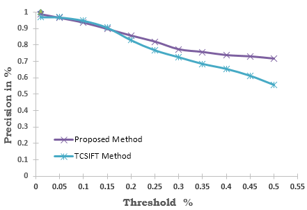
Figure 5. Line graph: Comparison of the proposed method vs. TCSIFT
The average retrieval/clustering rate of the proposed method was computed and compared with the TCSIFT method [15]. The retrieval/clustering rate of the proposed and the existing methods was diagrammatically represented in a Bar-chart, which is illustrated in Figure 5. It is observed from the line graph that the proposed method gives better precision than the TCSIFT method, and also it shows that there is no a significant change in the accuracy after a certain level of the distance threshold.
4.5 Computational complexity
The line graph indicates that the proposed method yields almost the same retrieval rate in terms of precision compared to TCSIFT method for the threshold less than or equals to 0.15, that is 15%. But, at the same time, one advantage of the proposed method is that it consumes lesser time than the TCSIFT method because the TCSIFT method requires complicated procedures to extract features. The proposed method consumes a minimum of a fixed amount of time for all threshold levels because first, it compares the median value of the key-frame with the median (index) value of each group of the feature vector database only. The median value has been indexed based on the median of each group/class. If the median value of the features vector of the key-frame matches, then only the proposed method takes into account of that group/class for the comparison of the features, otherwise it leaves the group/class and moves to the next one.
The proposed Big data-driven feature extraction method, based on statistical techniques, experimented with a video database. The video database contains more than 350 videos with 1279 clips collected from online resources such as YouTube and Metcalfe and from some movies that cover various scenarios like sports, films, advertisements, etc. Key-frames extracted from the videos stored in the video database; preprocesses, such as normalization, noise removal and, background scenes and foreground objects separation, were performed. The noise removed key-frames separated into background scenes and foreground objects. Features extracted from the background scenes and foreground objects separately. The extracted features formed as a feature vector, and the feature vectors clustered into a homogeneous group. The similar group of feature vectors indexed based on the median values of the group.
A key-frame inputted to the proposed system, which extracts feature as discussed above. The feature vector compared with the feature vectors of the feature vector database, based on the Canberra distance metric. The proposed feature extraction method matches and retrieves the video from the database. The proposed method gives 97.09% maximum of correct classification and 2.91% misclassification. The results obtained by the proposed method compared to the results of the TCSIFT methods. The comparative study reveals that despite the proposed method yields same or moderately better results than the TCSIFT method, the proposed method takes lesser time for feature extraction, matching, and retrieval of videos compared to the TCSIFT method. Also, the study shows that the obtained results are comparable with the existing methods.
The proposed method can be extended, in future, for feature extraction of share market trade data, and online multimedia data analytics. Also, the colour-based segmentation technique could be useful for shape detection of online multimedia data.
[1] Ferman, A.M., Tekalp, A.M., Mehrotra, R. (2002). Robust color histogram descriptors for video segment retrieval and identification. IEEE Transactions on Image Processing, 11(5): 497-508. https://doi.org/10.1109/TIP.2002.1006397
[2] Ning, J., Zhang, L., Zhang, D., Wu, C. (2009). Robust object tracking using joint color-texture histogram. International Journal of Pattern Recognition and Artificial Intelligence, 23(7): 1245-1263.
[3] Su, J.H., Huang, Y.T., Yeh, H.H., Tseng, V.S. (2010). Effective content-based video retrieval using pattern-indexing and matching techniques. Expert Systems with Applications, 37: 5068-5085. https://doi.org/10.1016/j.eswa.2009.12.003
[4] Ohta, Y.I., Kanade, T., Sakai, T. (1980). Color information for region segmentation. Computer Graphics and Image Processing, 13(3): 222-241. https://doi.org/10.1016/0146-664X(80)90047-7
[5] Charles, Y.R., Ramraj, R. (2016). A novel local mesh color texture pattern for image retrieval system. International Journal of Electronic Communication, 70: 225-233. https://doi.org/10.1016/j.aeue.2015.11.009
[6] Wang, H., Li, Z., Li, Y., Gupta, B.B., Choi, C. (2018). Visual saliency guided complex image retrieval. Pattern Recognition Letters, 130: 64-72. https://doi.org/10.1016/j.patrec.2018.08.010
[7] Chen, J., Zhao, G., Salo, M., Rahtu, E., Pietikäinen, M. (2013). Automatic dynamic texture segmentation using local descriptors and optical flow. IEEE Transactions on Image Processing, 22(1): 326-339. https://doi.org/10.1109/TIP.2012.2210234
[8] Ojala, T., Pietikäinen, M., Mäenpää, T. (2002). Multiresolution gray-scale and rotation invariant texture classification with local binary patterns. IEEE Transactions on Pattern Analyses and Machine Intelligence, 24(7): 971-987. https://doi.org/10.1109/tpami.2002.1017623
[9] Chen, J., Shan, S., He, C., Zhao, G., Pietikainen, M., Chen, X., Gao, W. (2010). WLD: A robust local image descriptor. IEEE Transactions on Pattern Analyses and Machine Intelligence, 32(9): 1705-1720. https://doi.org/10.1109/TPAMI.2009.155
[10] Dawood, H., Dawood H., Guo P. (2014). Texture image classification with improved weber local descriptor. Artificial Intelligence and Soft Computing. ICAISC 2014. Lecture Notes in Computer Science, vol 8467. Springer, Cham.
[11] Bhaumik, H., Bhattacharyya, S., Nath, M.D., Chakraborty, S. (2016). Hybrid soft computing approaches to content based video retrieval: A brief review. Applied Soft Computing, 46: 1008-1029. https://doi.org/10.1016/j.asoc.2016.03.022
[12] Galshetwara, G.M., Waghmarea, L.M., Gondea, A.B., Muralab, S. (2017). Edgy salient local binary patterns in inter-plane relationship for image retrieval in diabetic retinopathy. Procedia Computer Science, 115: 440-447. https://doi.org/10.1016/j.procs.2017.09.103
[13] Govindaraj, P., Sudhakar, M.S. (2018). Hexagonal grid based triangulated feature descriptor for shape retrieval. Pattern Recognition Letters, 116: 157-163. https://doi.org/10.1016/j.patrec.2018.10.004
[14] Harrouss, O.E., Moujahid, D., Tairi, H. (2015). Motion detection based on the combining of the background subtraction and spatial color information. 2015 Intelligent Systems and Computer Vision (ISCV), Fez, Morocco, pp. 1-4. https://doi.org/10.1109/ISACV.2015.7105548
[15] Zhu, Y., Huang, X., Huang, Q., Tian, Q. (2016). Large-scale video copy retrieval with temporal-concentration. SIFT. Neurocomputing, 187: 83-91. https://doi.org/10.1016/j.neucom.2015.09.114
[16] Ding, S., Qu, S., Xi, Y., Wan, S. (2019). A long video caption generation algorithm for big video data retrieval. Future Generation Computer Systems, 93: 583-595. https://doi.org/10.1016/j.future.2018.10.054
[17] Rautiainen, M., Seppdnen, T. (2005). Comparison of visual features and fusion techniques in automatic detection of concepts from news video. International Conference on Multimedia and Expo, Amsterdam, Netherland, pp. 932-935. https://doi.org/10.1109/ICME.2005.1521577
[18] Jansohn, C., Ulges, A., Breuel, T.M. (2009). Detecting pornographic video content by combining image features with motion information. ACM International Conference on Multimedia, Beijin, China, pp. 601-604. https://doi.org/10.1145/1631272.1631366
[19] Song, Y., Wang, W. (2009). Text localization and detection for news video. IEEE International Conference on Information and Computing Science, Manchester, UK, pp. 98-101. http://dx.doi.org/10.1109/ICIC.2009.133
[20] Lei, Z., Liu, Y., Zhang, W., Liu, X. (2012). A Nfl-based and feature extraction supported shot retrieval approach. 2nd International Conference on Computer Application and System Modeling, Hohhot, China, pp. 1072-1075. http://dx.doi.org/10.2991/iccasm.2012.272
[21] Cotton, C.V., Ellis, D.P.W. (2013). Subband autocorrelation features for video soundtrack classification. 38th International Conference on Acoustics, Speech, and Signal Processing, Vancouver, Canada, pp. 8663-8666. https://doi.org/10.7916/D8SF35G4
[22] Ali, H.H., Moftah, H.M., Youssif, A.A.A. (2018). Depth-based human activity recognition: A comparative perspective study on feature extraction. Future Computing and Informatics Journal 3(1): 51-67. https://doi.org/10.1016/j.fcij.2017.11.002
[23] Seetharamana, K., Palanivel, N. (2013). Texture characterization, representation, description, and classification based on full range Gaussian Markov random field model with Bayesian approach. International Journal of Image and Data Fusion, 4(4): 342-362. https://doi.org/10.1080/19479832.2013.804007
[24] Kokare, M., Chatterji, B.N., Biswas, B.K. (2003). Comparison of similarity metrics for texture image retrieval. TENCON 2003. Conference on Convergent Technologies for Asia-Pacific Region, Bangalore, India, 2: 571-575. https://doi.org/10.1109/TENCON.2003.1273228
[25] Mei, J.P., Chen, L. (2010). Fuzzy clustering with weighted medoids for relational data. Pattern Recognition, 43(5): 1964-1974. https://doi.org/10.1016/j.patcog.2009.12.007