A Novel ANN-ARMA Scheme Enhanced by Metaheuristic Algorithms for Dynamical Systems and Time Series Modeling and Identification

This section presents a brief explanation of the concept of ANN-ARMA and the metaheuristic algorithms used in building our proposed model.

2.1 ANN-ARMA Concept

Artificial neural networks are a field of artificial intelligence that attempts to emulate the functioning of the human neurological system in order to resolve complicated issues. ANN is made up of a large number of nodes known as artificial neurons. A weight and bias are assigned to each neuron, which indicates the information the network employs to solve a problem. Neurons are connected to one another through communication interactions. Inputs that a neuron receives determine its internal state or activation functions. A neuron’s activity is often sent as a signal to multiple other neurons. ANN changes the weights and biases of each neuron during training to minimize the difference between the expected and actual output using an optimization approach of gradient descent, which assesses the amount and direction of weight changes based on the error.

Autoregressive (AR) models and Moving Average (MA) models are commonly used in time series analysis. Autoregressive models predict the next value in a series based on the previous values, while the moving average models predict the next value based on the average of the previous values.

Artificial neural networks can also be used for time series analysis, including both autoregressive and moving average models. In an autoregressive ANN, the input to the network is a time series sequence, and the network uses previous values to predict the next value in the sequence. In a moving average ANN, the input to the network is a moving window of the time series sequence, and the network predicts the next value based on the average of the previous values in the window. A popular combination of these two approaches is the Autoregressive Moving Average (ARMA) model, which combines the strengths of both methods. In ARMA model, the network uses both the previous values and the moving average of previous values to predict the next value in the time series sequence. Autoregressive, moving average, and ARMA models can all be implemented using ANNs for time series analysis. The choice of which model to use depends on the particular characteristics of the time series data and objectives of analysis. For ARMA model, output is modelled as a linear difference equation between current and past inputs and past outputs as described in the equation that follows:

$y(t)=\sum_{i=1}^n a_i x(t-i)+\sum_{j=1}^n b_j u(t-j)$      (1)

where, $x(t)$ and $u(t)$ are inputs and outputs, $a_i$ and $b_j$ are the ARMA parameters.

Adding these outputs to a neural network as inputs is equivalent to changing its structure into a recurrent neural network. The objective of this hybrid structure (ANNARMA) is to combine the advantages of both and to obtain a more reliable modeling result.

In order to minimize the error between the model’s output and real data output, optimization algorithms are used to update the model’s parameters. Creating an appropriate fitness function, also known as an objective function, is essential for the effectiveness of the system identification and it is formulated to determine the control parameter values that best satisfy the desired goal. Usually, the control parameters must be selected within certain restrictive limits. In this work, Mean Square Error (MSE) criterion function was used which is described in the equation that follows:

$M S E=\frac{\sum_{K=1}^N\left(y_k-\hat{y}_k\right)^2}{N}$      (2)

where, $y_k$ and $\hat{y}_k$ are the actual measurement and its estimate, respectively, and $N$ is the length of the data.

2.2 Metaheuristic algorithms

In this section, we provide a synopsis of the IWO, PSO, ICA and CMA-ES metaheuristics algorithms.

2.2.1 Invasive weeds optimization

The population-based optimization approach known as "invasive weed optimization" (IWO) was first proposed by Mehrabian and Lucas in 2006, as stated in the study [26] and takes inspiration for solving continuous optimization problems from how invasive weeds operate in the natural world.

A significant threat to agricultural crops, weeds is distinguished by their strength, rapid adaption, and ability for propagation in the environment. Weeds invade fields by dispersing their seeds through the air. These seeds occupy the available spaces and grow into flowering weeds using the available resources. New weeds following the same process are randomly dispersed in the field and develop into the flowering weeds and the process continues.

The IWO algorithm is outlined below:

• Generate randomly a population of $n$  weeds.
• Generation of the seeds population.
• Evaluation of the fitness of each seed and rank them according to their fitness. The seeds now are called flowering weeds.
• Production of new seeds by the previous flowering weeds according to their rank. The number of seeds produced by a weed varies between $S_{\min }$ and $S_{\max }$ increasing linearly from the lowest ranked weed to the highest ranked weed.
• Generation of the seeds using the normally dispersed arbitrary numbers with mean equivalent to the location of the generating weeds. The standard deviations are varied according to the following equation:

$\theta_{\text {iter }}=\frac{\left(\text { iter }_{\max }-\text { iter }\right)^n}{\text { iter }_{\max }^n}\left(\theta_i-\theta_f\right)+\theta_f$      (3)

where, $iter_{\max }$ the maximum number of iterations, $\theta_i$ and $\theta_f$ are both the initial and the last standard deviations, and $n$ is the nonlinear modulation index.

• Evaluation of the fitness of newly generated seeds that become flowering weeds. They are then ranked with their parents according to their fitness.
• Elimination of weeds of lower fitness in order to attain the maximum number of weeds allowed in the colony $\left(P_{\max }\right)$.
• The survived weeds can produce new seeds according to their rank and this process continues until the stopping criterion is reached. The stopping criterion is usually considered to be the maximum number of iterations or a certain limit value of fitness.

2.2.2 Particle swarm optimization

Particle Swarm Optimization (PSO) is a forceful meta-heuristic optimization algorithm established by Kennedy and Eberhart in 1995 [27]. It was relying upon the comportment of flocking birds and schooling fish observed in nature. This algorithm works with this concept: a flock of birds is randomly initialized in the search area, where each bird is named a "particle". After a specific number of iterations, these birds (particles) locate the optimal global position. For each iteration, every particle is able to alter its velocity vector depending on its momentum and the effect of its best position as well as the best position of the most qualified individual. The particle then travels to a newly calculated location, and its fitness may be assessed using the optimization problem's objective function.  The particle's previously visited best position is marked as its personal best position ($P_{best}$). The global best position ($g_{best}$) is the location of the best person in the swarm. These two equations are used to assign the particle's velocity and new location at each step:

$\begin{aligned} & V_{(t+1)}=V_{(t)}+C_1 r_1\left(p b_{(t)}-X_{(t)}\right)+C_2 r_2\left(p g_{(t)}-X_{(t)}\right)\end{aligned}$      (4)

$X_{(t+1)}=X_{(t)}+V_{(t+1)}$      (5)

where, $C_1$ and $C_2$ are the acceleration coefficients, and $r_1, r_2$ are random variables in a range of $[0,1]$.

The PSO algorithm is described as follows:

• - Generate randomly a population swarm of $N$ particles.
• - Initialization of the parameters of PSO ($C_1$ and $C_1$).
• - Initialize particle with random position $(x)$ and velocity (v).
• - For each iteration, the following steps are repeated until satisfying the stopping criterion:

$\checkmark$  Solve the target problem.

$\checkmark$  Calculate the objective function.

$\checkmark$  Update the $g_{best}$ and $P_{best}$ values.

$\checkmark$  Update particle position $(x)$ and velocity $(v)$ according to the velocity and position updating Eqs. (4) and (5).

• - Stopping conditions are satisfied: $g_{b e s t}$ and optimal solution has been found.

2.2.3 Imperialist competitive algorithm

Imperialist Competitive Algorithm (ICA) is a socio-political metaheuristic algorithm proposed in 2007 by Atashpaz-Gargari and Lucas [28]. It was formed by the historical colonization process and the rivalry between empires for more colonies. The algorithm starts with a random initial population (country). The most powerful nation shall serve as the empire's imperialist, with the rest forming colonies. To assess the general intent of an empire, a linear combination of the imperialist's desired result and the average of the objective values of the empire's colonies is employed. The most vulnerable empire may be found after assessing all of the empires. Then all other empires compete to seize the weakest colony of the weakest empire.

The ICA algorithm is detailed as follows:

• Initialization of the algorithm.
• Generation of a collection of arbitrary solutions within the optimization problem's search space and create initial empires. Generation of random countries and determination of their power by the cost function.
• The countries having the cheapest function value turn Imperialists, seize control of other countries (or colonies), and establish the initial Empires.
• Assimilation induces each empire's colonies to move closer to the imperialist state in the space of seeking optimization.
• The revolution guides to sudden and random changes in the position of certain countries in the research space.
• Throughout assimilation and revolution, a colony may attain a better position and have the opportunity to take over the entire empire and replace the present imperialist state of the empire.
• For the imperialist competition, all empires compete to win the game and take control of colonies of other empires. Depending on their might, all empires have an opportunity of acquiring one or more colonies of the weaker empire at each stage of the algorithm.
• Until a stop condition is satisfied, the algorithm continues to progress through the above mentioned steps (Assimilation, Revolution, Competition).

2.2.4 Covariance matrix adaptation-evolution strategy

Covariance Matrix Adaptation Evolution Strategy (CMAES), as cited in the research, is a powerful version of evolution strategy algorithm for solving continuous optimization problems, introduced by Hansen and Ostermeier in 2001 [29]. CMA-ES is based on Evolution Strategy (ES) which is a type of evolution algorithm (EA). The mathematical and statistical model employed in the construction of CMA-ES is quite intriguing and sets it apart from all other evolutionary algorithms and metaheuristics. It consists in finding a vector of parameters $x$ that maximizes an objective or a fitness function $f(x)$. The mean and covariance of exploration distribution are ordinary variables and are not conditioned by the agent's current state.

Dynamic modifications to the search distribution are possible through the covariance matrix's adaptation mechanism, which sets CMA-ES unique. CMA-ES's unique characteristic significantly simplifies complex, high-dimensional objective function optimization. It has been successfully applied in many fields, including engineering, robotics, and other fields where conventional optimization techniques may falter, such as neural network architecture optimization and parameter tuning.

The CMA-ES is clarified below:

• Initialize the CMA-ES parameters.
• Generate a population of candidate solutions.
• Evaluate the fitness values for every individual in the population.
• Select parents from the fittest individuals, based on their fitness values, to establish the next generation's parent population.
• For each iteration, the following steps are repeated until satisfying the stopping criterion:

$\checkmark$  Update the Covariance Matrix:

$\begin{aligned} & C^{t+1}=\left(1-c_1-c_\mu\right) C^t+c_1+P_c^{t+1}\left(P_c^{t+1}\right)^T \\ & \quad+c_\mu \sum_{i=1}^\gamma W_{R i} \frac{X_i-m^t}{\sigma^t}\left(\frac{X_i-m^t}{\sigma^t}\right)^T\end{aligned}$      (6)

where, $c_1$ and $c_\mu$ are learning rate parameters, $W_{R i}$ is the weight for the $R^{\text {ith }}$ highest point, and $P_c$ is the evolution path.

$P_c^{t+1}=\left(1-C_c\right) P_c^t+\sqrt{\frac{C_c\left(2-C_c\right)}{\sum_{i=1}^\gamma W_i^2}} \frac{m^{t+1}-m^t}{\sigma^t}$      (7)

$\checkmark$  Update the Step Size:

$\sigma^{t+1}=\sigma^t \exp \left(\frac{c_\sigma}{d_\sigma} \frac{P_\sigma^{t+1}-X_d}{X_d}\right)$      (8)

where, $c_\sigma$ is the learning rate, $d_\sigma$ is the damping rate, and $P_\sigma$ is the evolution path.

$\checkmark$  Generate Sample Population for generation $t+1.$

$\checkmark$  Update the mean for generation $t+1$ :

$m^{t+1}=\sum_{i=1}^\gamma W_{R i} X_i $         (9)

$\checkmark$  Update the best-ever solution.

$\checkmark$  Stopping conditions are satisfied: Results.

In this section, we present and discuss the simulation results of the proposed method for modeling and identification of dynamical systems. For this purpose, the three nonlinear dynamical systems described below will be used for testing the ability of the proposed approach [16, 17]:

• System 1:

$\begin{gathered}y_p(k+1)=f\left[y_p(k), y_p(k-1), \ldots ., y_p(k-n\right. +1)]+\sum_{i=0}^{m-1} \beta_i u(k-1) \end{gathered}$      (11)

• System 2:

$y_p(k+1)=\Sigma_{i=0}^{n-1} \alpha_i y_p(k-1)+g[u(k), u(k-1), \ldots, u(k-m+1)]$      (12)

• System 3:

$\begin{gathered}y_p(k+1)=f\left[y_p(k), y_p(k-1), \ldots, y_p(k-n+1]\right. \\ +g[u(k), u(k-1), \ldots, u(k-m +1)]\end{gathered}$      (13)

Following an extensive comparative analysis, we have identified that the most effective optimization algorithm among the four utilized is the IWO algorithm. This will be showcased in the comparative study section. Subsequently, we will present the simulation results of our technique based on the IWO algorithm. The weights and the bias are parts of the proposed ANN model that can be tuned.  Below is a list of the various parameters of the IWO algorithm:

$\checkmark$  The Initial and final population size are 10 and 25, respectively.

$\checkmark$  The Minimum and maximum number of seeds are 0 and 5, respectively.

$\checkmark$  The Initial and final values of the standard deviation are 1.5 and -1.5, respectively.

4.1 Modeling and identification of system I

For this system, we consider the particular case governed by the following differential equation:

$y_p(k+1)=f\left[y_p(k), y_p(k-1)\right]+u(k)$      (14)

with:

$f\left[y_p, y_p(k-1)\right]=\frac{y_p(k) y_p(k-1)\left[y_p(k)+2.5\right]}{1+y_p^2(k)+y_p^2(k-1)}$     (15)

$u(k)=\sin \left(\frac{2 \pi k}{25}\right)$      (16)

where, $f$ is the part of Eq. (14) to be identified using the primary model, and $u$ is the input signal.

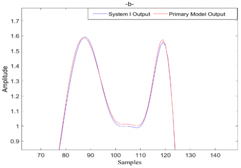
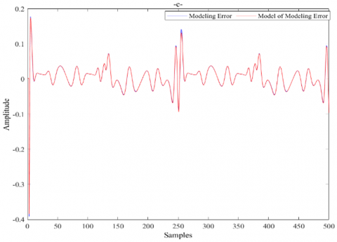
The simulation results of system I are presented in Figure 5, where,

$\checkmark$   Figure 5 (a): Superposition between the system I output and the primary model output.

$\checkmark$  Figure 5 (b): Zoomed segments of Figure 5 (a).

$\checkmark$  Figure 5 (c): Superposition between the modeling error and the model of modeling error.

$\checkmark$  Figure 5 (d): Superposition between the system I output and the final model output.

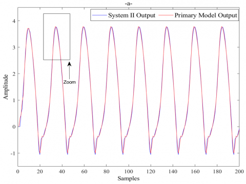
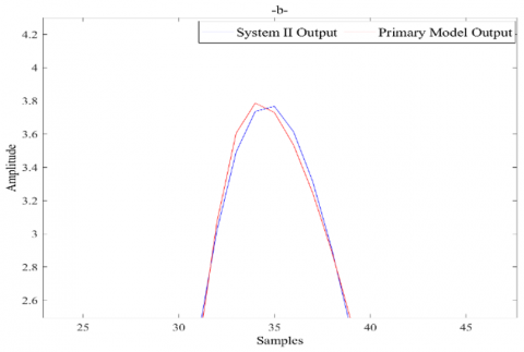
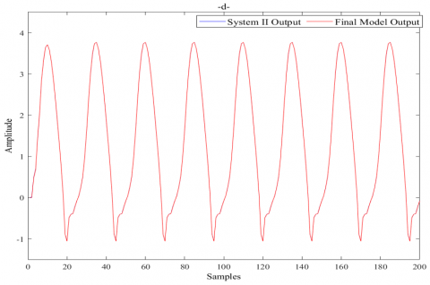
4.2 Modeling and identification of system II

For the second nonlinear dynamical system, the process to be determined is provided by the following difference equation:

$y_p(k+1)=0.3 y_p(k)+0.6 y_p(k-1)+f[u(k)]$      (17)

where, the following form represents the unknown function that has to be found:

$f(u)=0.6 \sin (\pi u)+0.3 \sin (3 \pi u)+0.1 \sin (5 \pi u)$      (18)

The input signal $u$  is chosen to be sinusoidal as follows:

$u(k)=\sin \left(\frac{2 \pi k}{250}\right)$      (19)

The same parameters of the IWO optimization algorithm as those used for system I are used to simulate the second system Modeling and identification, the simulation results are presented in Figure 6.

4.3 Modeling and identification of system III

For this system, we consider the particular case described by the following difference equation:

$\begin{aligned} & y_p(k+1)=f\left(y_p(k), u(k)\right) \\ & =\frac{y_p(k)}{1+y_p(k)^2}+u(k)^3\end{aligned}$      (20)

$u(k)=\sin \left(\frac{2 \pi k}{25}\right)+\sin \left(\frac{2 \pi k}{10}\right)$      (21)

where, $u(k)$ is the input signal. We simulated this case with the same parameters of the IWO optimization algorithm as with system I and system II. The simulation results are shown in Figure 7.

51.png

52.png

53.png

54.png

Figure 5. ANN-based IWO model for system I

61.png

62.png

63.png

64.png

Figure 6. ANN-based IWO model for system II

71.png

72.png

73.png

74.png

Figure 7. ANN-based IWO model for system III

A visual examination of all of these Figures 5-7 reveals that the ultimate model is greatly superior to the primary model. This observation verifies the usefulness of the error model-based identification idea.

4.4 Validation and generalization tests

To ensure both efficiency and robustness in our approach, validation tests have been conducted. A concise description of these validation tests is provided in this section.

4.4.1 Generalization test

The generalization process follows these steps: First, the primary model is validated using new input data $u_2$, resulting in a new error. Next, this error is utilized in the error identification step. Finally, the final model is generated, representing a concurrent interconnection involving two models (primary model and error model). The outcomes of the validation process are illustrated in Figure 8 where:

$\checkmark$  Figure 8 (a): represents the primary model output with the input data $u_1$ defined as follows:

$u_1(k)=\sin \left(\frac{2 \pi k}{25}\right)$      (22)

$\checkmark$  Figure 8 (b): represents the primary model output with the new input data $u_2$ given by the following equation:

$u_2(k)=\sin \left(\frac{2 \pi k}{25}\right)$ for $1 \leq k \leq 50$ and $150 \leq k \leq 200$      (23)

$u_2(k)=\sin \left(\frac{2 \pi k}{10}\right)+\sin \left(\frac{2 \pi k}{5}\right)$ for $50 \leq k \leq 150$      (24)

$\checkmark$  Figure 8 (c): represents the error process model.

$\checkmark$  Figure 8 (d): represents the final model output.

81.png

82.png

83.png

84.png

Figure 8. Generalization test

The generalization test for models is a crucial step in the evaluation of machine learning and statistical models. It assesses how well a trained model can perform on unseen or new data. Based on a visual examination of Figure 8 (d), it can be verified that our model demonstrates satisfactory performance on applying a new input, which confirms the effectiveness of our proposed approach.

4.5 Validation test

By conducting validation tests, we can assess the model’s reliability, generalization ability, and suitability for real-world applications. These tests are crucial in ensuring that the model is not only accurate on the data it was trained on but also effective in making predictions on new, unseen data.

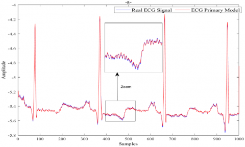
4.5.1 Modeling and identification of ECG signal

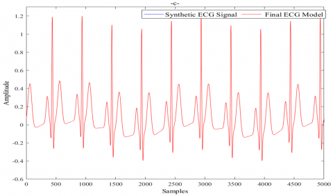
An ECG signal is a type of time series data which illustrates the heart's electrical activity over a particular period of time. In a time series, data points are recorded in chronological order at regular intervals. In the case of an ECG, the time series consists of a sequence of voltage measurements taken at successive time points during the cardiac cycle. In this section, our approach is applied to the identification of two types of ECG signals: Real ECG signals acquired from the ECG PhysioNet database [30] and synthetic ECG signal [31].

(1). Real ECG signal

In the following, we explore the implementation of the suggested approach on real ECG data. To conduct this study, we obtained the real ECG signal 100.dat dataset from the MIT-BIH normal sinus rhythm database [30], where it was recorded at a sampling rate of 360Hz with a resolution of 11 bits per sample. The outcome of applying the proposed method to the real ECG signal is visualized in Figure 9.

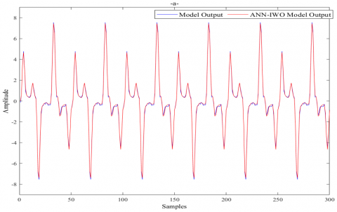
(2). Synthetic ECG signal

The same precepts and procedures used in the previous sections will be applied to model the synthetic ECG signal data [31]. The result gained is shown in Figure 10.

91.png

92.png

93.png

Figure 9. ANN based IWO model for real ECG signal: a) Real ECG signal vs Primary ECG model, b) the Modeling error vs Model of modeling error, c) the Real ECG signal vs the Final ECG model

10-1.png

10-2.png

10-3.png

Figure 10. ANN based IWO model for synthetic ECG signal: a) synthetic ECG signal vs Primary ECG model, b) Modeling error vs Model of Modeling error, c) synthetic ECG signal vs Final ECG model

4.5.2 Mackey-Glass time series modelling and identification

Remember that a time series is only a set of data points organized temporally. Our method is also used to additional data from a time series. Time often serves as the independent variable in a time series, and future forecasting is the main goal. We take into consideration a time series produced by the Mackey-Glass equation for this purpose. Figure 11 shows the simulation's results.

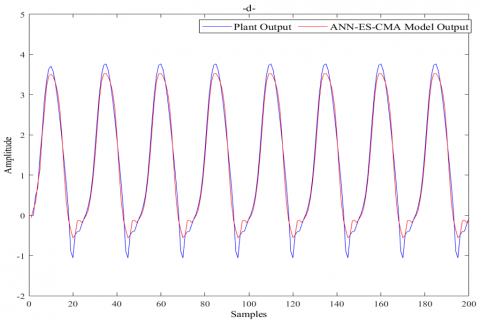
4.6 Comparative study

In this section, a comparison is conducted to demonstrate the efficacy of the IWO optimization algorithm in contrast to other optimization techniques. To accomplish this, we have selected three algorithms, namely PSO, ICA, and ES-CMA, as described in section.1.2. The specific parameters for each optimization algorithm are chosen as follows: PSO algorithm parameters (the acceleration constants $C_1=1.5, C_2=2.5$ and the coefficient of inertia $\omega=0.48 )$, ICA algorithm parameters $(\alpha=1, \beta=1.5, \mu$ (revolution rate) $=0.1)$, ESCMA algorithm parameters ( $\lambda$ (Population size) $=140$, $\mu($ Number of Parents $)=40 )$. Figures 12-14 depict the modeling and identification results of the three dynamical systems mentioned earlier, employing the proposed modelling method based on the four-optimization algorithms (IWO, PSO, ICA, and ES-CMA).

After analysing all the figures, it is evident that the IWO algorithm exhibits superior performance when compared to the PSO, ICA, and ES-CMA algorithms. The results indicate that the IWO algorithm outperform the other optimization techniques in terms of Modeling and identification of the dynamical systems under consideration.

11-1.png

11-2.png

11-3.png

Figure 11. ANN based IWO model for Mackey Glass time series: a) Mackey Glass time series vs Primary model, b) Modeling error vs Model of Modeling error, c) Mackey Glass time series vs Final model

12-1.png

12-2.png

12-3.png

12-4.png

Figure 12. System I based ANN model: (a) IWO, (b) PSO, (c) ICA, (d) ES-CMA

13-1.png

13-2.png

13-3.png

13-4.png

Figure 13. System II based ANN model: (a) IWO, (b) PSO, (c) ICA, (d) ES-CMA

14-1.png

14-2.png

14-3.png

14-4.png

Figure 14. System III based ANN model: (a) IWO, (b) PSO, (c) ICA, (d) ES-CMA

Currently, we proceed with a numerical evaluation of the method’s performance using a fitness function known as the mean square error (MSE). To ensure reliability, we conducted 20 independent trials of our method and for each optimization algorithm. Table 1 presents statistical performance measures, including the worst and best values of the fitness function.

Table 1. The fitness function results for 20 independent trials

Optimization Algorithm	Best Value	Worst Value
IWO	9.1127e-9	8.1002e-7
PSO	8.2201e-6	5.9317e-4
ICA	4.2138e-6	1.2139e-5
ES-CMA	4.2138e-6	1.7293e-5

Based on Table 1 and out of the techniques discussed, the IWO (Invasive Weed Optimization) algorithm demonstrated superior performance by achieving the best value across the 20 independent trials.

Moreover, to conduct comprehensive statistical investigations, we incorporated error bars for parameter optimization. This graphical technique represents the variability of the estimated parameters on graphs, providing an indication of the uncertainty associated with estimates and offering a general understanding of the parameter’s values accuracy. The primary model’s error bars parameters and the error process Modeling parameters can be observed in Figures 15 and 16, respectively.

A simple visual inspection of these figures, indicating that the error bars widths associated with the IWO method are the smallest when compared to the error bars of the PSO method, the ICA method, and CMA methods. This finding suggests that the IWO method exhibits greater precision and consistency in parameter optimization.

15-1.png

15-2.png

15-3.png

15-4.png

Figure 15. Primary model parameters error bars: (a) IWO, (b) PSO, (c) ICA, (d) ES-CMA

16-1.png

16-2.png

16-3.png

16-4.png

Figure 16. Error process parameters error bars: (a) IWO, (b) PSO, (c) ICA, (d) ES-CMA

4.7 Discussion

Our approach, which combines ANN and IWO methods and incorporates an error model, improves the modeling and identification of dynamical systems and time series significantly. By combining ANN and IWO, we increase efficiency and produce better solutions in situations where traditional methods may fail. This collaboration between ANN and IWO not only improves the ability to solve complex problems, but also enables us to deal with difficult scenarios more effectively. Our findings have a significant impact because they provide better predictions and optimization strategies for real-world tasks in fields such as finance and engineering. Our adaptable method is a valuable tool for control and decision-making in dynamical systems, making it applicable across industries and allowing us to address complex challenges effectively.