Gowtham Rajendiran*![]() | Jebakumar Rethnaraj
| Jebakumar Rethnaraj![]()
© 2024 The authors. This article is published by IIETA and is licensed under the CC BY 4.0 license (http://creativecommons.org/licenses/by/4.0/).
OPEN ACCESS
The rise in agricultural innovation has led to the use of sustainable farming practices, such as aeroponics, which increase crop production. Aeroponics, a soil-free indoor precision farming system, cultivates crops using vertical towers, garnering global attention for its environmentally friendly and productive cultivation methods. Aeroponic systems can grow lettuce, a popular green-leafy vegetable, quickly and with minimal water usage. However, yield prediction is a tedious task in real-world scenarios. To efficiently predict lettuce yield, various scientific experiments have integrated IoT and machine-learning techniques. This research work utilized various machine-learning regression models, including linear, support vector, random forest, and XGBoost, to estimate lettuce yield based on specific growth parameters such as pH, EC, temperature, total dissolved salts (TDS), turbidity, humidity and light. After implementation, the results showed a high prediction accuracy of 93% and minimal error rates produced by the XGBoost regression model when compared with the other regression models. Further, fine-tuning the model parameters enhanced the XGBoost model's performance, enhancing its generalization capability to handle new real-time data. This indicates that optimizing the lettuce yield involves not only using indoor aeroponic farming methods but also utilizing advanced sustainable food production systems.
aeroponics, artificial intelligence (AI), indoor farming, internet of things (IoT), lettuce, machine learning regression, vertical farming, yield prediction
The increasing population, climate change, and food constraints have led to a growing interest in alternative farming methods like hydroponics and aeroponics. These methods offer year-round harvests, weather protection, easy transportation, support for various crop cultivars, and disease-free practices, making them crucial for addressing food security concerns in the global economy. Aeroponics, a soilless method with an innovative tower structure, has shown significant improvements in crop yields ranging from 7% to 65%, accelerated crop maturation rates, and optimized water, pesticide and fertilizer consumption patterns when compared to the traditional farming techniques [1, 2].
Soil-free cultivation uses hydroponic or aeroponic systems to grow plants without soil. Hydroponics involves submerging roots in nutrient solutions, while aeroponics aerosolizes the solution. These systems offer a controlled environment and easy nutrient manipulation, making them ideal for genetic studies and screening mutant phenotypes. Aeroponic systems are more efficient due to their ability to suspend roots in mist, improve oxygen exposure, and produce fine particles [3-5].
Artificial Intelligence (AI) has shown potential for improving crop yield predictions in fields like healthcare, robotics, and meteorology. It can enhance efficiency and accuracy in agricultural yield prediction by optimizing parameters like light exposure, nutrient supply, and temperature [2, 6-8]. In aeroponic systems, the utilization of AI techniques like machine learning algorithms plays a vital role, especially in data analysis, real-time growth monitoring, resource management and predictive modeling.
The study stresses how important it is to accurately predict aeroponic crop yields in modern farming. This lets farmers use advanced machine learning algorithms to make the best use of their resources, come up with effective farming strategies, and cut down on losses [9, 10]. Accurate yield prediction in aeroponic systems is crucial for food production and resource management. It optimizes factors like yields, crop appearance, nutritional content, quality, and taste while minimizing resource usage like nutrients, water, and energy, leading to effective cost utilization and optimized resource utilization.
Real-time aeroponics systems require improved decision-making processes and accuracy in yield prediction models to address the aforementioned factors, which have been elaborated on in this research work. The structure of this document comprises four sections: Section 2 provides an overview of existing works, while Section 3 details the methods used to collect and analyze data, including the implementation of machine learning models and interpretability techniques. Section 4 presents the findings and their implications, while Section 5 summarizes key takeaways and potential areas for further research.
The literature survey on lettuce yield predictions in aeroponic vertical farming systems using machine learning regression algorithms is a critical examination of precision agriculture research. The survey focuses on lettuce cultivation in aeroponic vertical farming and aims to identify trends, methodologies, and key findings in predictive modeling for yield outcomes. The comprehensive exploration not only establishes the theoretical foundation for future research but also contributes insights for developing robust predictive models tailored to the unique challenges and opportunities presented by aeroponic vertical farming in lettuce cultivation.
Nutrient sensors detect and measure plant environment and data transmitted through wireless networks, determining the necessary nutrients for plant growth, such as nitrogen, phosphorus, and potassium, which are crucial for vertical or closed crop cultivation [11].
The study introduces the Lettuce Crop Development Monitoring-Boost (LCGM-Boost) regression model, which improves lettuce crop monitoring and predicts yield in aeroponic vertical farming systems. The model considers pH, EC, PPM, turbidity, and temperature parameters. It shows robustness against outliers, superior prediction accuracy, and reduced error rates. This model is suitable for automating lettuce crop growing settings and predicting yield [12].
Aeroponics, a soilless farming technique, has been significantly transformed by technology, offering environmental control, automated nutrient delivery, and plant health monitoring. The most common technology is sensing technology and Industry 4.0, offering sustainability and time efficiency. However, technical complexity and power dependency pose challenges. The Technology Adoption and Integration in Sustainable Agriculture (TAISA) model assesses technology integration in sustainable agriculture systems. Asia leads in technology integration, with Indonesia being the most studied country. As technology advances, careful consideration of benefits and limitations will lead to more efficient, productive, and resilient aeroponic cultivation systems [13].
The study assesses the use of Support Vector Regression (SVR) in estimating crop yields using the LCGMS Regression model, revealing environmental factors affecting crop growth. It suggests future research should focus on improving evaluation indices and data features for evidence-based decision-making, food security, and sustainable agricultural practices [14].
The authors have developed a meta-heuristic optimization technique for diagnosing heart disease using sound waves. The method uses Particle Swarm Optimization, the Firefly approach, and the Cuckoo Search Algorithm to find the most optimal feature vector. The approach is evaluated on the Pascal dataset, which is divided into separate sets for testing and training. Machine learning methods like Random Forest, K-Nearest Neighbors, Support Vector Machines, and Naive Bayes are used. The model achieved the highest classification accuracy of 90.32% using CSA and Naive Bayes [15].
The article suggests using shape curvature and multi-feature fusion for weed identification in crops. Shape curvature is useful for shape-based identification, while texture features provide discriminatory information. Combining both is advantageous. The SVM classifier outperformed other classifiers with 99.33% classification accuracy, potentially benefiting autonomous weed management systems by reducing false negative rates [16].
The study presents a high-throughput architecture for detecting anomalies in streaming data using the Apache-Kafka-powered model. The RF algorithm achieves average accuracy, precision, recall, f-score, and computation time values of 98.6%, 91.8%, 90.4%, 91.09%, and 38.5ms, respectively. However, it exhibits over-fitting tendencies when dealing with small-sized data. The architecture's ability to channel data without data loss and consistent accuracy make it feasible for real-life applications [17].
A machine learning framework has been developed to assess students' satisfaction with online admissions counseling. The framework uses a Decision Tree Classifier without SMOTE and SVC-linear using SMOTE to estimate satisfaction rates. The accuracy was achieved at 48% in the Decision Tree Classifier without and 88% in SVC-linear using SMOTE, allowing for the optimization of students' choices based on their strengths, weaknesses, and related parameters [18].
Franchetti et al. [19] used 3D plant modeling and deep segmentation techniques to forecast the plant growth of Basil phenotyping with the help of features plant height, leaf area, and leaf weight where the accuracy was moderate. In another article, the authors used random forest and SVM for predicting rosette phenotyping with the help of plant leaves as a feature [20]. The LSSVM machine learning framework was proposed to find the water stress of the wheat crop. Here, the plant leaf was used as an essential feature [21]. Techniques like Self-Organizing Maps (SOM), hierarchical clustering, and k-means algorithm were utilized for lettuce crop growth prediction with the extracted feature plant leaf and achieved higher accuracy rates [22]. Data visualization and Logistic regression approaches were used for analyzing the distribution of the dataset of the lettuce crop and produced the average error rates while predicting the lettuce yield [23]. In Mamatha and Kavitha [24], K nearest neighbors were implemented for predicting the yield of leafy vegetables which used the plant growth as the feature vector and produced a higher prediction accuracy. Reinforcement learning has been adopted by the authors for finding the phenotyping of the crops chili, beans, potatoes, and onions with a prediction accuracy of 83.563%. This work extracted plant leaves as the observed features for learning purposes [25]. The authors in the article [26] analyzed the effectiveness of the random forest regression model in predicting the aeroponic lettuce crop yield.
So, from all these previous researches, it is inferred that most of the authors have utilized the applications of integrated IoT and ML algorithms without any doubts. Hence, the comparatives of those ML algorithms with their specific advantages have been carried out by the authors in this manuscript to provide which model is better for predicting aeroponic lettuce crop yield.
This section deals with the prediction of growth stages and harvesting of the Lactuca Sativa i.e. botanical name of lettuce crop. The yield prediction usually involves two different methodologies, 1) manual and 2) technology-driven approach. Both techniques are explained in brief in the following sub-sections. To increase lettuce crop production through vertical aeroponic systems, this research examines a twofold methodology that blends conventional techniques (manual or traditional) with advanced technology (technology-driven applications) to accurately predict yields. Given the distinctive features of aeroponic systems, it is crucial to adopt an integrated approach that combines tried-and-true agricultural practices with state-of-the-art tools to achieve optimal results.
Table 1. Comparison between manual and technological approaches in yield prediction
|
Parameters |
Manual Approach |
Technology-Driven Approach |
|
Data Collection |
Conventional methods involve collecting data through visual evaluations of plant health, nutrient availability, and growth patterns, allowing researchers to identify and document key factors for qualitative analysis. |
Sensor technology like Internet of Things devices and environmental sensors provide real-time quantitative data on crop growth variables, ensuring continuous observation and increased accuracy in information gathering. |
|
Model Developments |
Prediction models are enhanced by the addition of experts' subject knowledge. In building models, leaf color, size, and general health of plants are taken into account along with information gathered manually. |
ML algorithms process sensor data to identify complex patterns, and analyze ensemble techniques, neural networks, or regression models, providing lettuce yield estimates as a quantitative framework. |
|
Performance Evaluation |
Agricultural specialists conduct qualitative analysis to evaluate model effectiveness, based on their extensive expertise, to evaluate the models' usefulness and applicability. |
ML models' accuracy and efficacy are evaluated using quantitative measures like mean squared error and R-squared values, providing a basis for identifying reliable prediction algorithms. |
3.1 Predicting the yield of aeroponic lettuce-manual and technology-driven methods
The basic comparison of predicting yield using manual and with the help of technology is presented in the form of Table 1.
3.2 Machine learning in lettuce yield prediction
With their advanced analytical ability to cope with the complexity of agricultural systems, machine learning (ML) algorithms have become a potent tool in the prediction of lettuce crop yields. Here, in this work, we have utilized different machine-learning regression models that provide a greater impact on the yield prediction of the lettuce crop.
3.2.1 Utilized machine learning models
Linear Regression. Linear regression is the fundamental and interpretable machine learning regression model used for predicting numerical values with the help of the linear equation. In an aeroponic lettuce crop yield prediction system, the model estimates the linear relationship between the one input variable and the output variable. It is mathematically represented as:
$y=m x+b$ (1)
where, y is the dependent variable (crop yield), x is the independent variable (input parameters), m is the slope and b is the intercept term.
Multiple Linear Regression Model. Linear regression models are simple approaches used to find the relationships between two variables, the input, and the output variable. But for more complex relationships that require more consideration, the multiple linear regression models were highly utilized to find the relationships between the multiple input variables and the output variable i.e. the situation where multiple independent variables are used to estimate the outcome of the single dependent variable. There are two main uses of this regression analysis: 1) to determine the dependent variable based on the multiple independent variables and 2) to determine how strong the relationship is between the variables.
Multiple linear regression is often used when forecasting more complex relationships. In an aeroponic lettuce crop yield prediction system, multiple regression models can make effective predictions on the new and unseen data. The coefficients of the feature variables are determined which allows the growers to make informed decisions about the crop behavior and yields. Equation 2 is the mathematical representation of the MLR:
$y=b_0+b_1 x_1+b_2 x_2+\cdots+b_n x_n$ (2)
where, $y$ is the dependent variable (crop yield), $\left[x_1, x_2, \ldots, x_n\right]$ is the independent variable (input parameters) and $\left[b_0, b_1, b\right.$ $\left.2, \ldots, b_{\mathrm{n}}\right]$ are the coefficients.
Support Vector Regression. Support Vector regression is a type of supervised machine learning algorithm that works similarly to that of the SVM algorithm. The model aims to minimize the errors in the actual and predicted values which fit the hyper plane into the data points. In an aeroponic lettuce yield prediction system, the dependent variable lettuce yield is predicted using the independent variables which are the environmental factors for growing the lettuce crop with the help of different kernel functions to fix the non-linearities into linear problems. It deals with the complex relationship between the environmental factors and the yield. SVR allows hyper-parameter tuning which improves the accuracy of the prediction model to better fit into the dataset. Like other regression models, SVR can be iteratively improved by incorporating the new and the unseen data.
The mathematical formulation of the SVR objective function involves defining a hyperplane that finds the relationship between the input parameters and the output (yield). The data points n concerning the input parameters Xi and the corresponding output (yields) yi, where, i=1, 2, 3, …, n the SVR objective function could be written as two different equations as represented below.
i) In the case of linear kernel
$min _{w, b, \zeta, \zeta^*} \frac{1}{2} w^T w+C \sum_{i=1}^n\left(\zeta_i+\zeta_i^*\right)$ (3)
subject to the constraints $=\left(y_i-w^T X_i-b \leq \varepsilon+\zeta_i\right)\left(w^T X_i+\right.$ $\left.b-y_i \leq \varepsilon+\zeta_i^*\right)$ where, $\zeta_i, \zeta_i^* \geq 0$.
ii) In the case of a non-linear kernel
$min _{w, b, \zeta, \zeta^*} \frac{1}{2} w^T w+C \sum_{i=1}^n\left(\zeta_i+\zeta_i^*\right)$ (4)
subject to the constraints $=\left(y_i-\phi\left(X_i\right)^T w-b \leq \varepsilon+\right.$ $\left.\zeta_i\right)\left(\phi\left(X_i\right)^T w+b-y_i \leq \varepsilon+\zeta_i^*\right)$ where, $\zeta_j, \zeta_i^* \geq 0$.
where, $\phi\left(X_i\right)$ is the transformation of $X_i$ into a highdimensional space.
In these equations, $w$ and $b$ are the parameters to be learned from the training data, $\zeta_{\mathrm{i}}$ and $\zeta_i^*$ are slack variables allowing for deviations from the actual output and $C$ is a regularization parameter controlling the trade-off between model simplicity and accuracy.
Random Forest Regression. The Random Forest (RF) is the collection and utilization of multiple decision trees for output predictions. It is the ensemble learning approach that combines the output of multiple weak learners to improve the accuracy and robustness of the model. Each decision tree deals with the subset of random features that promotes the diversity leading to the chances of better predictions. It has the capability of handling missing values which does not require any external preprocessing techniques. Also, the model could effectively handle larger datasets. In an aeroponic vertical farming system, the RF supports the complex interaction between the dependent and the independent features. One of the main advantages of RF regression is that it handles the overfitting problem due to the randomness in the feature selection. With the help of feature importance, the growers were able to gain insights into the input parameters that have the most significant impact on the lettuce yield.
It is represented as the average of individual tree predictions which is given below:
$\hat{y}(X)=\frac{1}{N} \sum_{i=1}^N F_i(X)$ (5)
where, $\hat{y}(X)$ is the predicted output (yield) for the given set of input parameters $(X), N$ is the number of trees in the random forest, $F_i(X)$ is the prediction output from $i^{\text {th }}$ decision tree.
Here, each tree $F_i(X)$ is constructed based on the random subset of features at each split. The final prediction is an average of these individual tree predictions.
XGBoost Regression. The Extreme Gradient Boosting-XGBoost model is a powerful machine learning algorithm that excels in real-world prediction tasks. It uses a decision-tree-based ensemble model to reduce errors and improve accuracy. The learning rate is used to control the behavior of each decision tree, affecting the overall model's accuracy. The model is effective in aeroponic lettuce crop yield prediction, handling missing values, non-linearities, and complex relationships, and preventing overfitting. It also focuses on feature importance, identifying environmental factors, and ensuring sufficient resource allocation and decision-making by growers. The model learns patterns and predicts outcomes effectively with new data.
Assuming the dataset with n observations and m features and predicting a continuous output variable y based on the input features X, the XGBoost regression model is given by:
$\widehat{y}_l=\phi\left(x_i\right)=\sum_{k=1}^K f_k\left(x_i\right)$ (6)
where, $\widehat{y}_l$ is the predicted output for observation $i$, $\phi\left(x_i\right)=$ $\sum_{k=1}^K f_k\left(x_i\right)$ is the ensemble prediction for observation $i$, $f_k\left(x_i\right)$ is the prediction of the $k^{\text {th }}$ regression tree.
The individual regression tree prediction, fk(xi) is constructed based on the sum of predictions from each tree node along with the path that observation i takes down the tree.
$f_k\left(x_i\right)=w_{q_{(i, k)}}$ (7)
where, $w_{q_{(i, k)}}$ is the weight associated with the terminal node $q_{(\mathrm{i}, k)}$ that observation $i$ reaches in the $k^{\text {th }}$ regression tree.
Hence, the overall objective function for the XGBoost regression model is the sum of a regularized training loss and the regularization term:
$\operatorname{obj}(\theta)=\sum_{i=1}^n L\left(y_{i,} \widehat{y}_l\right)+\sum_{k=1}^K \Omega f_k$ (8)
where, $\theta$ represents the parameter of the model; $L\left(y_{i,} \widehat{y}_l\right)$ represents the training loss of the observation $i$ and $\Omega \mathrm{f}_{\mathrm{k}}$ is the regularization term for the $k^{\text {th }}$ regression tree. Here, important to note that is, the training loss is often MSE for the regression trees.
3.3 Systematic representation of lettuce yield prediction
The systematic representation or the workflow diagram is represented in Figure 1. It is the collection of different modules used to describe the stepwise implementation of the proposed system. In other words, it is the encapsulation of the workflow that provides a clear-cut graphical illustration of the implementation procedure. It improves communication and provides an easy understanding of the underlying mechanism.
Figure 1. Lettuce crop yield prediction system
From Figure 1, it is clear that the implementation procedure starts with data collection and proceeds with the series of processes towards the yield prediction as the outcome. The detailed description of the various processes is explained below.
3.3.1 Data collection and data visualization
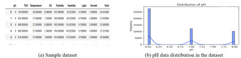
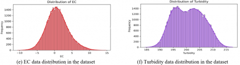
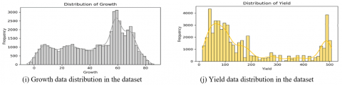
The first and foremost step in the implementation procedure is the data collection. Here, sensors such as pH sensor, EC sensor, temperature sensor, total dissolved salts (TDS) sensor, turbidity sensor, humidity sensor, and light sensor were deployed in the aeroponic lettuce growth tower. The data were collected from the growth tower at regular intervals of time, sample data is represented in the Figure 2. To easily understand the data distributions, data visualization techniques like bar charts (univariate data representation technique), correlogram (bivariate data analysis technique), and Andrews curve were utilized and implemented using the Python packages with the help of Python programming language.
From Figure 2 (a-j), the input parameters are represented individually with the help of bar plots.
Correlogram of the input dataset highlights the correlation between the input variables. Here, in Figure 2(l), the considered lettuce growth parameters were less correlated with the other parameters. This showcases that the parameters are independent of each other i.e. one cultivation parameter will not affect another parameter which is necessary for efficient lettuce growth and yield prediction.
Figure 2. Sample dataset and dataset visualization techniques
3.3.2 Data preprocessing
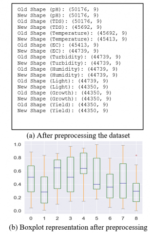
One of the most important steps in the machine learning implementation is the pre-processing of the dataset for efficient prediction output. Here, in the aeroponic lettuce crop yield prediction system, the outliers are the major cause of higher error rates and low prediction accuracy. Hence, the removal of the outlier’s mechanism is incorporated for effective prediction by the regression models. The dataset size is represented below before pre-processing as the old shape and after pre-processing as the new shape of the dataset.
Figure 3. Data preprocessing
The boxplot represents the dataset after pre-processing. The x-axis provides the different features of the lettuce growth dataset i.e. [0-8] is [pH to Yield] collected from the aeroponic vertical farming tower which is highlighted in Figure 3 (a) and (b).
3.3.3 Dataset splitting
Once the data is collected, pre-processed and ready for the implementation process, there is a necessary step called data partitioning or splitting of the data, before the data is fed into the ML model. In the case of the efficient implementation of the classification or regression model, the data has to be split into two: training data and testing data as shown in Figure 4.
Figure 4. Dataset splitting
3.3.4 Machine learning implementation: Model training and model testing
The actual work of the implementation phase begins now. A structured methodology is used to train and evaluate machine learning regression models for predicting aeroponic lettuce crop yields. The collected, analyzed and pre-processed datasets were fed into all four machine-learning models for training purposes. Once, the training of the models is done, next comes the testing phase. The test dataset is supplied to the trained machine learning models for testing the performance of the models. The testing scores were recorded and based on the produced results, the process called hyper-parameter tuning is carried out to achieve better results further. The detailed description of the results produced by the models was described in the results and discussions section.
4.1 System requirements
The system requirements that are essential to carry out the result analysis were the Anaconda Navigator, Jupyter Notebook with the Python programming language, and the desktop system or the personal computer or the laptop with the storage provided in the system or the laptop.
In this section, the detailed notes on the performance of different machine learning models were described elaborately. The best model was chosen based on the error rates and the prediction accuracy produced by the model, i.e. how accurately the regression model predicts the yield of the lettuce crop in the aeroponic environment.
4.2 Evaluation of the ML models using the performance metrics along with performance analysis
Performance metrics are the fundamentals used for assessing the performance of the machine learning regression models based on the produced prediction output from the actual values and interpreting the accuracy of the predictions. The most commonly used evaluation metrics in lettuce yield prediction analysis are listed below.
4.2.1 Mean squared error (MSE)
It is the average of the squared differences between the predicted values (xi) and the actual values (yi). It penalizes larger errors more heavily.
$M S E=\frac{1}{n} \sum_{i=1}^n\left(y_i-x_i\right)^2$ (9)
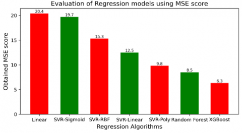
The MSE score of the implemented models is given in Table 2 and Figure 5.
Table 2. MSE scores
|
Regression Type |
MSE |
|
|
Linear (Multiple) |
20.4 |
|
|
Support Vector Regressor Kernels |
Sigmoid |
19.7 |
|
RBF |
15.3 |
|
|
Linear |
12.5 |
|
|
Poly |
9.8 |
|
|
Random forest |
8.5 |
|
|
XGBoost |
6.3 |
|
Figure 5. Graph for MSE score
All these regression models produce different error rates and linear regression shows less performance accuracy when compared to other regression algorithms.
4.2.2 Root mean squared error (RMSE)
It is the square root of the MSE. It provides the measure of the average magnitude of the errors in the predicted values, in the same units as the response variable.
$R M S E=\sqrt{M S E}$ (10)
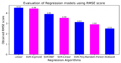
The RMSE score of the implemented models is given in Table 3 and Figure 6.
The XGBoost regression algorithm produced a minimum rmse score than the other regression algorithms. Next random forest regression algorithm produces an error rate less than the other five regression algorithms. The maximum rmse score is produced by the linear regression model.
Table 3. RMSE scores
|
Regression Type |
RMSE |
|
|
Linear (Multiple) |
4.516 |
|
|
Support Vector Regressor Kernels |
Sigmoid |
4.438 |
|
RBF |
3.911 |
|
|
Linear |
3.535 |
|
|
Poly |
3.13 |
|
|
Random forest |
2.915 |
|
|
XGBoost |
2.509 |
|
Figure 6. Graph for RMSE score of the utilized models
4.2.3 Mean absolute error (MAE)
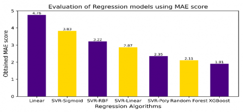
It computes the average absolute differences between the predicted (xi) and the actual values (yi), providing the measure of the average magnitude of errors. The MAE score is highlighted in Table 4 and Figure 7.
$M A E=\frac{1}{n} \sum_{i=1}^n\left(y_i-x_i\right)$ (11)
Table 4. MAE scores
|
Regression Type |
MAE |
|
|
Linear (Multiple) |
4.765 |
|
|
Support Vector Regressor Kernels |
Sigmoid |
3.832 |
|
RBF |
3.215 |
|
|
Linear |
2.867 |
|
|
Poly |
2.353 |
|
|
Random forest |
2.107 |
|
|
XGBoost |
1.906 |
|
Figure 7. MAE Scores of the utilized models
4.2.4 Mean absolute percentage error (MAPE)
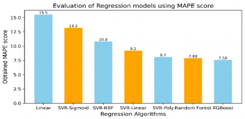
The MAPE expresses the errors as a percentage of the actual values, providing a relative measure of accuracy. Below presented Table 5 and Figure 8 highlights the obtained MAPE scores of the model.
$M A P E=\frac{1}{n} \sum_{i=1}^n\left(\frac{y_i-x_i}{y_i}\right) \times 100$ (12)
Table 5. MAPE scores
|
Regression Type |
MAPE |
|
|
Linear (Multiple) |
15.5 |
|
|
Support Vector Regressor Kernels |
Sigmoid |
13.2 |
|
RBF |
10.8 |
|
|
Linear |
9.2 |
|
|
Poly |
8.1 |
|
|
Random forest |
7.89 |
|
|
XGBoost |
7.581 |
|
4.2.5 Median absolute percentage error (MedAPE)
It is the median of the absolute percentage errors, making it less sensitive to outliers than MAPE.
$MedAPE=$ median $\left(\frac{y_i-x_i}{y_i}\right) \times 100$ (13)
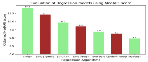
The MedAPE score of the implemented models is given in Table 6 and Figure 9:
Table 6. MedAPE scores
|
Regression Type |
MedAPE |
|
|
Linear (Multiple) |
14.2 |
|
|
Support Vector Regressor Kernels |
Sigmoid |
12.1 |
|
RBF |
9.7 |
|
|
Linear |
8.5 |
|
|
Poly |
6.9 |
|
|
Random forest |
6.3 |
|
|
XGBoost |
4.8 |
|
Figure 9. MedAPE scores of the utilized models
4.2.6 Root mean square logarithmic error (RMSLE)
It is the measure of the average difference between the logarithm of the predicted (xi) and the actual values (yi). It is particularly useful when the target variable has a wide range.
$R M S L E=\sqrt{\frac{1}{n} \sum_{i=1}^n\left[\left(1+y_i\right)-\log \left(1+x_i\right)\right]^2}$ (14)
Table 7. RMSLE scores
|
Regression Type |
RMSLE |
|
|
Linear (Multiple) |
1.876 |
|
|
Support Vector Regressor Kernels |
Sigmoid |
1.83 |
|
RBF |
1.76 |
|
|
Linear |
1.4 |
|
|
Poly |
1.253 |
|
|
Random forest |
1.176 |
|
|
XGBoost |
1.03 |
|
The RMSLE score of the implemented models was given in Table 7 and Figure 10:
Figure 10. RMSLE scores of the utilized models
4.2.7 R-squared metrics (Coefficient of determination)
R-squared metrics represent the proportion of the variance in the independent variable that is predictable from the independent variable. Usually, this metric ranges between 0 and 1. A higher R-squared value indicates a better fit of the model to the data.
$R^2=\left[1-\frac{\sum_{i=1}^n\left(y_i-\hat{y}_l\right)^2}{\sum_{i=1}^n\left(y_i-\underline{y}\right)^2}\right]$ (15)
Table 8. R-squared scores
|
Regression Type |
R-Squared |
|
|
Linear (Multiple) |
0.574 |
|
|
Support Vector Regressor Kernels |
Sigmoid |
0.676 |
|
RBF |
0.679 |
|
|
Linear |
0.768 |
|
|
Poly |
0.792 |
|
|
Random forest |
0.8154 |
|
|
XGBoost |
0.8948 |
|
Figure 11. R-squared scores of the utilized models
The R-squared score of the implemented models is given in Table 8 and Figure 11.
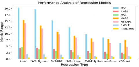
4.3 Comparative analysis of the performance metrics
The performance analysis of all the utilized ML models has been done in this sub-section. Various results produced were depicted in the Table 9 and Figures 12, 13.
Figure 12. Performance graph of the utilized regression models
All these models are compared individually only with my collected dataset. Based on the results produced (refer Table 9, Figure 12 and Figure 13) by linear regression, Support Vector Regressor with their kernels: sigmoid, linear, radial basis function (RBF) and polynomial, random forest and XGBoost regression, it is observed that there is a consistent improvement in the predictive performance and decrease in the error metrics respectively. It should be noticed that a higher value of 0.89 R-squared metrics is shown by the XGBoost regression model.
Figure 13. Accuracy of the utilized models
4.4 Prediction graphs
The graphs that showcase the predictive performance of the supervised and unsupervised machine learning classification and regression models by describing the complex relationships between the original (actual) values and the predicted values are termed prediction graphs. These graphs are used to perform a comprehensive analysis of various prediction algorithms to depict the efficacy of each algorithm separately. These graphs, not only highlight the individual strengths of each model but also contribute valuable insights for understanding the applicability of each model in predicting the complex relationships between the variables or parameters within the dataset.
Table 9. Consolidated evaluation metrics of the ML models
|
Regression Type |
MSE |
RMSE |
MAE |
MAPE |
MedAPE |
RMSLE |
R-Squared |
Prediction Accuracy in % |
|
|
Linear (Multiple) |
20.4 |
4.516 |
4.765 |
15.5 |
14.2 |
1.876 |
0.574 |
64.92 |
|
|
Support Vector Regressor Kernels |
Sigmoid |
19.7 |
4.438 |
3.832 |
13.2 |
12.1 |
1.83 |
0.676 |
68.51 |
|
RBF |
15.3 |
3.911 |
3.215 |
10.8 |
9.7 |
1.76 |
0.679 |
71.46 |
|
|
Linear |
12.5 |
3.535 |
2.867 |
9.2 |
8.5 |
1.4 |
0.768 |
78.74 |
|
|
Poly |
9.8 |
3.13 |
2.353 |
8.1 |
6.9 |
1.253 |
0.792 |
83.647 |
|
|
Random forest |
8.5 |
2.915 |
2.107 |
7.89 |
6.3 |
1.176 |
0.8154 |
87.538 |
|
|
XGBoost |
6.3 |
2.509 |
1.906 |
7.581 |
4.8 |
1.03 |
0.8948 |
92.865 |
|
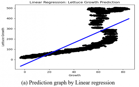
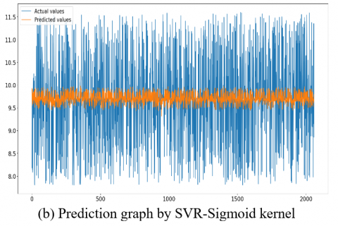
Figure 14. Prediction Graphs of the utilized models
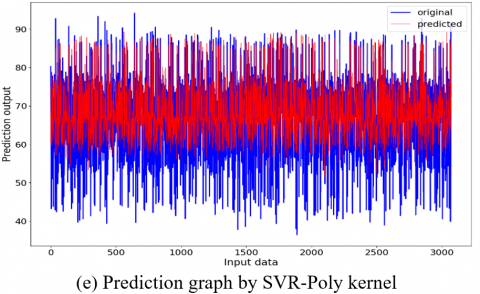
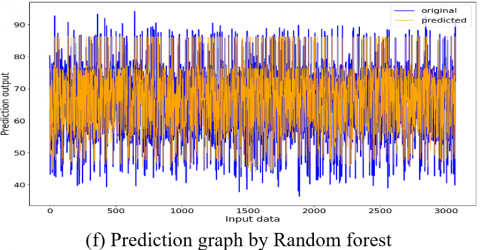
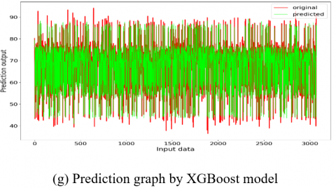
In this research work, Figure 14 (a) linear regression prediction graph highlights the linear relationship between the input parameters (actual values) and the output parameter (predicted values). From Figure 14, it is clear that the prediction accuracy gradually increases from support vector kernel- sigmoid, rbf, linear to polynomial kernel. These kernels exhibit distinctive patterns across each kernel which represents the average fit of the dataset and enhances the model’s ability to capture the non-linearities. Next comes the random forest and the XGBoost regressors that showcase remarkable accuracy, illustrating their robustness to outliers and noise by capturing the complex relationships within the dataset.
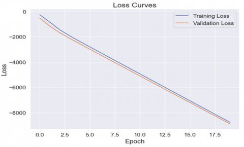
4.5 Choosing the best model using the training and validation loss curves
In simple terms, both these curves: the training loss curve and validation loss curves are crucial in machine learning regression as these curves showcase the generalization ability of the ML model on the unseen data i.e., the model should have the capability to generate the same type of output produced on the seen data (to predict the lettuce crop yield in our case) when it is exposed to the unseen dataset from the external environment.
Figure 15. Training and validation loss
In summary, the purpose of the study was to optimize lettuce crop growth by integrating precision agriculture practices with intelligent techniques. Also, the results comprehensively analyzed the performance of several machine learning regression models in the context of a vertical aeroponic farming system to make accurate predictions of lettuce production. We have gained valuable insights into their effectiveness in handling the complex interactions between environmental variables such as pH, EC, temperature, total dissolved salts (TDS), turbidity, humidity, light and growth in days that are inherent to aeroponic cultivation as a result of our in-depth analysis and comparison of models such as linear regression, support vector regression, and random forest regression. This was accomplished through rigorous analysis and comparison of these models.
According to the findings of our research, XGBoost surpasses the others in terms of error rates, accuracy and predictive power, demonstrating its potential as an excellent option for the prediction of lettuce production in aeroponic vertical farming. However, it is crucial to note that there are multiple aspects of agricultural systems and the selection of the most appropriate model may change depending on certain environmental conditions. This is something that has to be acknowledged.
This research work makes a significant contribution to the expanding body of knowledge in the field of precision agriculture, specifically the aeroponics indoor farming systems by providing practical recommendations on the application of machine learning regression models to the problem of maximizing the output of lettuce grown in aeroponic conditions. The research work enhances crop prediction in vertical farming systems, paving the way for future research and technology interventions to improve agricultural practices, reduce environmental impact, and enhance crop production. It also encourages competition in crop markets by incorporating diversification and crop rotation strategies, minimizing resource usage and promoting short-term growth while minimizing pests, diseases, and climatic variability.
The future development of the Aeroponic Lettuce Yield Prediction System is focused on enhancing its accuracy and reducing errors. This involves investigating various factors such as environmental conditions, nutrient levels, plant growth patterns, and more. In addition, the team plans to employ advanced machine learning techniques like ensemble learning and data augmentation to optimize model performance. Real-time sensor data integration and leveraging pre-trained models are also part of the roadmap to further boost prediction capabilities. To make the system easy to use for farmers and operators, an intuitive interface with clear visualizations and actionable insights will be implemented.
[1] Chandra, S., Khan, S., Avula, B., Lata, H., Yang, M.H., ElSohly, M.A., Khan, I.A. (2014). Assessment of total phenolic and flavonoid content, antioxidant properties, and yield of aeroponically and conventionally grown leafy vegetables and fruit crops: A comparative study. Evidence-based Complementary and Alternative Medicine, 2014: 253875. https://doi.org/10.1155/2014/253875
[2] Jiang, J.A., Liao, M.S., Lin, T.S., Huang, C.K., Chou, C.Y., Yeh, S.H., Lin, T.T., Fang, W. (2018). Toward a higher yield: A wireless sensor network-based temperature monitoring and fan-circulating system for precision cultivation in plant factories. Precision Agriculture, 19: 929-956. https://doi.org/10.1007/s11119-018-9565-6
[3] Jensen, M.H. (1997). Hydroponics. HortScience HortSci, 32(6): 1018-1021. https://doi.org/10.21273/HORTSCI.32.6.1018
[4] Velazquez-Gonzalez, R.S., Garcia-Garcia, A.L., Ventura-Zapata, E., Barceinas-Sanchez, J.D.O., Sosa-Savedra, J.C. (2022). A review of hydroponics and the technologies associated with medium and small-scale operations. Agriculture, 12(5): 646. https://doi.org/10.3390/agriculture12050646
[5] Lakhiar, I.A., Gao, J., Syed, TN., Chandio, F.A., Buttar, N.A. (2018). Modern plant cultivation technologies in agriculture under controlled environment: A review on aeroponics. Journal of Plant Interactions, 13(1): 338-352. https://doi.org/10.1080/17429145.2018.1472308
[6] Castro Zunti, R., Chae, K.J., Choi, Y., Jin, G.Y., Ko, S.B. (2021). Assessing the speed-accuracy trade-offs of popular convolutional neural networks for single-crop rib fracture classification. Computerized Medical Imaging and Graphics, 91: 101937. https://doi.org/10.1016/j.compmedimag.2021.101937
[7] Wang, Y., Choi, E.J., Choi, Y., Zhang, H., Jin, G.Y., Ko, S.B. (2020). Breast cancer classification in automated breast ultrasound using a multiview convolutional neural network with transfer learning. Ultrasound in Medicine & Biology, 46(5): 1119-1132. https://doi.org/10.1016/j.ultrasmedbio.2020.01.001
[8] Wang, Y., Zhang, H., Chae, K.J., Choi, Y., Jin, G.Y., Ko, S.B. (2020). Novel convolutional neural network architecture for improved pulmonary nodule classification on computed tomography. Multidimensional Systems and Signal Processing, 31: 1163-1183. https://doi.org/10.1007/s11045-020-00703-6
[9] Lakhiar, I.A., Jianmin, G., Syed, T.N., Chandio, F.A., Buttar, N.A., Qureshi, W.A. (2018). Monitoring and control systems in agriculture using intelligent sensor techniques: A review of the aeroponic system. Journal of Sensors, 2018: 1-18. https://doi.org/10.1155/2018/8672769
[10] Barker, D.G., Pfaff, T., Moreau, D., Groves, E., Ruffel, S., Lepetit, M., Journet, E.P., et al. (2006). Growing M. truncatula: Choice of substrates and growth conditions. The Medicago truncatula handbook, 1-26.
[11] Tipwong, W., Chongjarearn, Y., Sirikham, A., Preutisrunyanont, O. (2022). A novel determination of an appropriate clustering quantity of a water-soluble NPK nutrient measuring system based on K-means and SOM methods. In 2022 International Electrical Engineering Congress (IEECON), pp. 1-4. https://doi.org/10.1109/iEECON53204.2022.9741588
[12] Rajendiran, G., Rethnaraj, J. (2023). Smart aeroponic farming system: Using IoT with LCGM-Boost regression model for monitoring and predicting lettuce crop yield. International Journal of Intelligent Engineering & Systems, 16(5): 251-262. https://doi.org/10.22266/ijies2023.1031.22
[13] Garzón, J., Montes, L., Garzón, J., Lampropoulos, G. (2023). Systematic review of technology in aeroponics: Introducing the technology adoption and integration in sustainable agriculture model. Agronomy, 13(10): 2517. https://doi.org/10.3390/agronomy13102517
[14] Gowtham, R., Jebakumar, R. (2023). A machine learning approach for aeroponic lettuce crop growth monitoring system. In International Conference on Intelligent Sustainable Systems, pp. 99-116. https://doi.org/10.1007/978-981-99-1726-6_9
[15] Isik, I. (2023). Heart disease prediction with feature selection based on metaheuristic optimization algorithms and electronic filter model. Arabian Journal for Science and Engineering, 1-14. https://doi.org/10.1007/s13369-023-08515-z
[16] Agarwal, D. (2024). A machine learning framework for the identification of crops and weeds based on shape curvature and texture properties. International Journal of Information Technology, 16(2): 1261-1274. https://doi.org/10.1007/s41870-023-01598-9
[17] Surianarayanan, C., Kunasekaran, S., Chelliah, P.R. (2024). A high-throughput architecture for anomaly detection in streaming data using machine learning algorithms. International Journal of Information Technology, 16(1): 493-506. https://doi.org/10.1007/s41870-023-01585-0
[18] Shibli, A.R., Fatima, N., Sarim, M., Masroor, N., Bilal, K. (2023). Machine learning-based predictive modeling of student counseling gratification: A case study of Aligarh Muslim University. International Journal of Information Technology, 16: 1909-1915. https://doi.org/10.1007/s41870-023-01620-0
[19] Franchetti, B., Ntouskos, V., Giuliani, P., Herman, T., Barnes, L., Pirri, F. (2019). Vision-based modeling of plant phenotyping in vertical farming under artificial lighting. Sensors, 19(20): 4378. https://doi.org/10.3390/s19204378
[20] Lee, U., Chang, S., Putra, G.A., Kim, H., Kim, D.H. (2018). An automated, high-throughput plant phenotyping system using machine learning-based plant segmentation and image analysis. PloS one, 13(4): e0196615. https://doi.org/10.1371/journal.pone.0196615
[21] Moshou, D., Pantazi, X.E., Kateris, D., Gravalos, I. (2014). Water stress detection based on optical multisensor fusion with a least squares support vector machine classifier. Biosystems Engineering, 117: 15-22. https://doi.org/10.1016/j.biosystemseng.2013.07.008
[22] Alejandrino, J., Concepcion, R., Lauguico, S., Tobias, R.R., Almero, V.J., Puno, J.C., Bandala, A., Dadios, E., Flores, R. (2020). Visual classification of lettuce growth stage based on morphological attributes using unsupervised machine learning models. In 2020 IEEE Region 10 Conference (TENCON), pp. 438-443. https://doi.org/10.1109/TENCON50793.2020.9293854
[23] Gowtham, R., Jebakumar, R. (2023). Analysis and prediction of lettuce crop yield in aeroponic vertical farming using logistic regression method. In 2023 International Conference on Sustainable Computing and Data Communication Systems (ICSCDS), pp. 759-764. https://doi.org/10.1109/ICSCDS56580.2023.10104763
[24] Mamatha, V., Kavitha, J.C. (2023). Machine learning-based crop growth management in greenhouse environment using hydroponics farming techniques. Measurement: Sensors, 25: 100665. https://doi.org/10.1016/j.measen.2023.100665
[25] Obu, U., Sarkarkar, G., Ambekar, Y. (2021). Computer vision for monitor and control of vertical farms using machine learning methods. In 2021 International Conference on Computational Intelligence and Computing Applications (ICCICA), pp. 1-6. https://doi.org/10.1109/ICCICA52458.2021.9697152
[26] Rajendiran, G., Rethnaraj, J. (2023). Lettuce crop yield prediction analysis using random forest regression machine learning model in aeroponics system. In 2023 Second International Conference on Augmented Intelligence and Sustainable Systems (ICAISS), pp. 565-572. https://doi.org/10.1109/ICAISS58487.2023.10250535