Abdelouafi Boukhris*![]() | Antari Jilali
| Antari Jilali![]() | Hiba Asri
| Hiba Asri![]()
© 2024 The authors. This article is published by IIETA and is licensed under the CC BY 4.0 license (http://creativecommons.org/licenses/by/4.0/).
OPEN ACCESS
Crop diseases present a major threat to agricultural output, disrupting both the quantity and quality of production. Disease diagnosis remains a challenge for farmers, primarily due to limited knowledge and the need for specialized agricultural engineering expertise. To solve these problems, a new technique named the Autoencoder Latent Space-Neural Network (ALS-NN) was introduced in this study. It combines the strengths of autoencoders and neural networks to find crop diseases. Data processing is the first step of the methodology, and then data compression into a latent space follows. This compressed data serves as the input for the neural network, facilitating efficient crop disease classification. This approach capitalizes on the autoencoder's capacity for dimensionality reduction, data compression, and encoding, which is particularly beneficial when handling high-dimensional data. The reduced data dimensionality enables the neural network to process the information more efficiently. The ALS-NN model, by compressing data, focuses on the crucial information for the classification process, thereby enhancing computational speed and reducing the number of trained parameters. This results in time efficiencies during disease detection operations, mitigating the detrimental effects of diseases on crop yields. The integration of autoencoders and neural networks forms a potent strategy for disease detection, leveraging the autoencoders' capabilities for dimensionality reduction, anomaly detection, and feature learning, coupled with the classification and generalization abilities of neural networks. This hybrid approach can potentially lead to more precise, efficient, and interpretable disease detection system. PlantVillage is used with 10 crop types. We used the first part of autoencoder (The encoder) to compress images into Latent space; for classification, the result is subsequently fed into a neural network. Our model (ALS-NN) achieved 90% for test accuracy and 90% for validation accuracy.
neural network, autoencoder, latent space, encoder, deep learning
Crops are susceptible to various types of diseases which can effectively reduce production and negatively affect the agriculture economies. The problem of crop diseases is a significant and ongoing challenge in agriculture worldwide. Crop diseases can have catastrophic impacts on food production, leading to decreased yields, economic losses for farmers, and potential food shortages. These diseases are caused by different pathogens, including fungi, bacteria, viruses, and pests, which can infect a wide range of crops, from staple grains like wheat and rice to fruits like apples and citrus. Effective disease management is important to guarantee food security and sustainable agricultural applications.
Morocco is an agricultural country and produces several types of crops like tomato, potato, wheat, and pepper. That’s why we worked on tree types of crops which are: Peppers, Potatoes and Tomatoes, and eight types of diseases which are: bacterial spot which affect pepper, potato early and light blight and tomato diseases (target spot, mosaic virus, yellow leaf curl, bacterial spot and early blight). To address these issues, we must detect early and automatically crop diseases. Many research works presented varied state-of-the-art systems for crop diseases identification using machine learning and deep learning algorithms. Nandhini and Ashokkumar [1] uses DenseNet-121 for plant leaf disease identification, Shadin et al. [2] use convolutional neural network and Inception V3 COVID-19 diagnosis from chest X-ray images, Khan et al. [3] use SqueezeNet to classify diseases in citrus fruits and the accuracy was 96%, Bharathi and Sonai [4] uses convolution encoder method to detect leaf disease and the accuracy was 98%.
The state-of-the-art techniques are time consuming and use a high trainable parameters number, so a machine with high computational power is required. So, we need a novel model which can reduce the training time significantly and the number of training parameters.
The main contribution of our novel model is shown as follows:
(1) Data processing: after loading data from PlantVillage dataset, we resize all images and normalize them which can accelerate the convergence rate and improve the robustness of our proposed method.
(2) We built our variational autoencoder to encode the prepared data by Encoder, which can represent our data in low dimension called Latent Space or Bottleneck. This step compresses our data to speed up the training of our network.
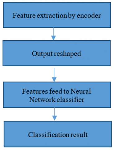
(1) We reshaped all compressed data to use them for our neural network.
(2) The Encoder output serves as the input for our deep neural network.
(3) Deep neural network identifies crop disease.
We used TensorFlow to build our model that could identify crop disease with good accuracy using the dataset PlantVillage. We have tree steps in our proposed model. The first step is data processing, the PlantVillage dataset is preprocessed by resizing images, cutting and normalization of data to improve the model accuracy Khamparia et al. [5]. Second step, we built our variational autoencoder to encode the dataset images and project all images in Latent Space. The third step, we train our neural network with the features extracted by our encoder. We used Adam optimizer algorithm for training which can enhance the learning efficiency of our model and leads to faster convergence of loss function. For ten kinds of diseases the model accuracy achieved 90% which demonstrates the effectiveness of our proposed model.
Several methods have already been used to accurately identify crop diseases through image classification. In all these methods, they have used several image processing methods like SVM, Neural Network (NN), K-mean algorithms and so on.
Bharathi and Sonai proposed a system to detect crop leaf disease using convolutional encoder architecture. They combined variational autoencoder for data extraction and convolutional neural networks for classification, this method named V-Convolution encoder network reached an accuracy of 98% after 150 epochs and with a convolution filter of 3*3.
Another work has been done by Khamparia et al. [5] where they used a convolutional neural network based autoencoder for crop leaf diseases detection, they have proposed hybrid technique to detect leaf diseases combining CNN and autoencoders. The dataset used contains 900 images. The accuracy of this approach reached 97.5% after 100 epochs.
Using five CNN architectures, Sanga et al. [6] proposed a banana disease identification system. They found that ResNet-152 outperformed all other architectures and the accuracy was 99.2%.
Chohan et al. [7] used Inception and VGG-19 architecture for plants disease identification using PlantVillage dataset. They found that VGG-19 outperformed Inception V3 with accuracy of 95% and 98% for testing and training respectively.
Mohameth et al. [8] combined various architectures to detect plant disease. For features extraction they used CNN architectures and for classification they employed k-Nearest Neighbor and Support Vector Machine (SVM) classifiers. The experiment shows that SVM and CNN combined reached an accuracy of 98% which outperformed all others.
Another similar work, for plant disease identification, has been done by Tiwari et al. [9] which combined various CNN architectures for features extraction, such as VGG-16, VGG19 and Inception V3, and classifiers like NN, SVM, KNN and Logistic Regression. After experiment, they observed that combining Logistic Regression with VGG-19 reached an accuracy of 97.8%.
Sibiya and Sumbwanyambe [10] use CNN for maize disease classification, Türkoğlu and Hanbay [11] combined three classifiers K-Nearest Neighbor, Extreme Learning Machine, and Support Vector Machines with state-of-the-art model (SqueezeNet, ResNet-50, ResNet-101, Inception-v3, InceptionResNetv2, and GoogLeNet) for plant disease recognition. Too et al. [12] presented a comparative study to select the best deep learning model for crop disease detection.
Pardede et al. [13] combined Convolutional Autoencoder (CAE) with SVM for corn and potato diseases identification. They used CAE architecture for features extraction and SVM for classification. Using PlantVillage dataset this proposed work achieved an accuracy of 87.01% and 80.42% for potato and corn diseases identification respectively. Ferentinos [14] use five CNN architecture to detect plant disease. Table 1 summarizes various research work using PlantVillage dataset.
Table 1. Some of the proposed works by the authors
|
Name |
Year |
Proposed Work |
Result |
|
Nandhini and Ashokkumar [1] |
2022 |
DenseNet-121 |
|
|
Shadin et al. [2] |
2021 |
CNN and InceptionV3 |
|
|
Khan et al. [3] |
2021 |
SqueezeNet |
|
|
Bharathi and Sonai [4] |
2022 |
variationalautoencoder combined with CNN |
98% |
|
Khamparia et al. [5] |
2020 |
CNN+Autoencoder [15] |
97.5 % |
|
Sanga et al. [6] |
2020 |
ResNet-152 |
99.2% |
|
Chohan et al. [7] |
2020 |
VGG-19 |
98% |
|
Mohameth et al. [8] |
2020 |
Combination of SVM and ResNet-50. |
98% |
|
Tiwari et al. [9] |
2020 |
Combination of Logistic Regression and VGG-19. |
97.8% |
|
Pardede et al. [13] |
2018 |
Convolutional Autoencoder (CAE) combined with SVM |
87.01% |
Most of these works mentioned above had a high training time. That’s why we are motivated to strive towards building a model that can reduce the training time and detect crop disease with a good classification accuracy as much as possible.
The significant advantage of ALS-NN is training time reduction and the number of training parameters is also reduced.
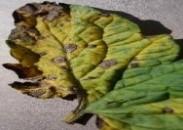
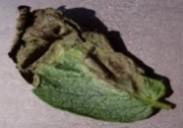
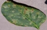
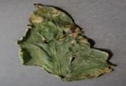
The first task of this step is loading data from the PlantVillage dataset, we collected images of ten crop diseases which are mostly affected diseases in Morocco. These are Potato Early blight, Late blight, Tomato Target Spot, Tomato mosaic virus, Tomato Yellow Leaf Curl Virus, Tomato Bacterial spot, Tomato Early blight. Examples of our dataset are displayed in Table 2 with disease name. The PlantVillage comprises a total of 54,303 images of leaves, which are further categorized into 38 different groups based on factors like the plant species and the presence of diseases. The dataset is usually organized into subfolders or directories, with each subfolder representing a specific plant disease or plant type. Within each subfolder, you will find images of plants belonging to that category. For example, there might be subfolders named "Tomato_Healthy," "Tomato_Early_Blight," "Potato_Late_Blight," and so on. Here's a simplified example of how the dataset might be structured:
PlantVillage_Dataset/
Tomato_Healthy/
image1.jpg
image2.jpg
...
Tomato_Early_Blight/
image1.jpg
image2.jpg
...
Potato_Late_Blight/
image1.jpg
image2.jpg
...
...
The dimension of each image is 256*256 and all images are typically stored in common image formats, such as JPEG or PNG.
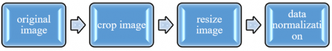
To speed up our model and achieve a good accuracy we must process data. The first step in data processing is image cropping without reducing images quality. Second step is image resizing to have the desired size of our model which is 60x60 pixel. We also used some data augmentation techniques like random flipping and horizontal and vertical translation. After that we normalize the data to speed up the rate of convergence and for similarity distribution of data. Figure 1 illustrates the steps of data processing.
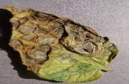
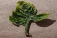
Table 2. PlantVillage dataset samples
|
Infected Images |
Disease Name |
|
Tomato Early blight |
|
|
Potato Late blight |
|
|
Pepperbell Bacterial spot |
|
|
Tomato Bacterial spot |
|
|
Potato Early blight |
|
|
Tomato Yellow Leaf |
Figure 1. 4 Steps to process data
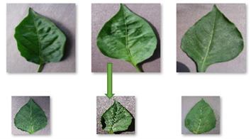
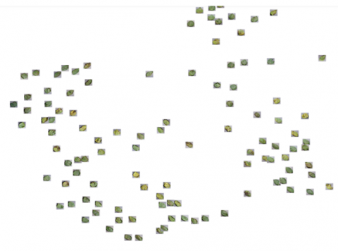
Figure 2 illustrates some data examples after cropping and resizing images:
Figure 2. Leaf images after cropping and resizing operation
We will discuss in this section the techniques used to design our novel model. Section 4.1 offers a fundamental concept of the Autoencoder and Neural Network. In section 4.2 we detailed our hybrid system. Section 4.3 provides the experimental setup to implement our novel system.
4.1 Algorithms used
This part outlines Vanilla Autoencoder and Deep Neural Network architecture.
4.1.1 Autoencoder
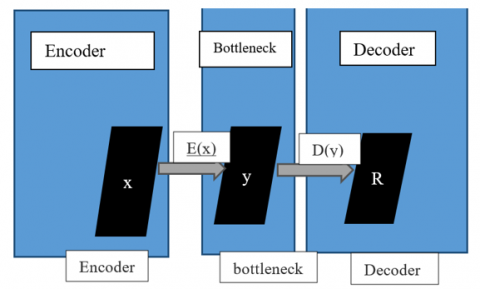
Autoencoder is a deep learning algorithm used on feature selection and extraction, based on unsupervised learning, and uses backpropagation algorithms to learn the weight parameters of the network. The output and input vectors have the same dimensionality because the network reconstructs its own inputs after training process. Figure 3 shows the pipeline of an autoencoder:
Figure 3. Pipeline of an autoencoder
Autoencoder compress data into lower representation named bottleneck or code and tries to reconstruct the output from the bottleneck. An autoencoder have three components: Encoder, code (or bottleneck or Latent-Space) and Decoder. The objective of the Encoder is to compress data into low dimension named code or Latent-Space (or bottleneck). Encoder is a Neural Network which contains many layers; the last layer is the bottleneck layer. We assume that we have N layers; The equation bellow (1) shows the operation of each Encoder layer:
$X_{e i+1}=f_{e_i}\left(W_{e_i}^T X_{e_i}+b_{e_i}\right) \forall i=0,1,2, \ldots, N$ (1)
For the ith Encoder layer:
Xei: is the input; Xei+1: the result; Wei: the weight; bei: the bias; fei: the activation function.
In general, the Encoder can be represented by the mathematical function bellow:
$z=f(W x+b)$ (2)
where, Z is the latent dimension (code), f is the activation function, W and b are weight and bias respectively.
The decoder reconstructs the input based on latent space. The input of the Decoder is the output of bottleneck layer (code). The Decoder can be represented by the following equation:
$X_{d i+1}=f_{d_i}\left(W_{d_i}^T X_{d_i}+b_{d_i}\right) \forall i=0,1,2, \cdots, N$ (3)
For the ith Decoder layer:
Xdi: the input; Xdi+1: the result; Wdi: the weight; bdi: the bias; fdi: the activation function.
In general, the Decoder can be represented by the mathematical function bellow:
$x^{\prime}=f^{\prime}\left(W^{\prime} z+b^{\prime}\right)$ (4)
The difference between the reconstructed data XR and the original data XO is called Reconstruction Loss (RL). To minimize the RL, we used backpropagation algorithm to train the autoencoder. To compute the RL, we can use two loss functions which are BCE and MSE. The mathematical equations for these two-loss functions shown in (5) and (6):
$\operatorname{MSE}\left(X^O, X^R\right)=\frac{1}{D} \sum_{j=1}^D\left(X_j^O-X_j^R\right)^2$ (5)
$B C E\left(X^O, X^R\right)=-\frac{1}{D} \sum_{j=1}^D X_j^O \cdot \log X_j^R+\left(1-X_j^O\right) \cdot \log \left(1-X_j^R\right)$ (6)
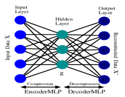
Vanilla autoencoder proposed by LeCun et al. [16] contain only one hidden layer with a number of neurons less than the number of neurons in the input and output layer. The hidden layer is considered as a bottleneck layer which restricts and minimizes the information that would be stored. The main goal of Vanilla autoencoder is to learn how to develop a compressed input at the Latent Space layer. Figure 4 bellow illustrates the architecture of Vanilla autoencoder:
Figure 4. Architecture of vanilla autoencoder
Vanilla autoencoder:
A vanilla autoencoder, often referred to simply as an "autoencoder," is a kind of artificial neural network employed for unsupervised learning and dimensionality reduction. It's called "vanilla" to distinguish it from more complex variations like convolutional autoencoders or recurrent autoencoders.
Here's a breakdown of the components and purpose of a vanilla autoencoder:
·Encoder: is the first part of the autoencoder. Encodes data into a lower-dimensional representation. This lower-dimensional representation is often referred to as the "encoding" or "latent space.".
·Bottleneck Layer: The bottleneck layer, which is part of the encoder, is where the dimensionality reduction occurs. The number of neurons is fewer than the number of neurons in the input layer. This forces the network to capture the most essential features of the input data while discarding less important details.
·Decoder: The decoder is the second part of the autoencoder. It takes the encoded data and attempts to recreate the original input as closely as possible.
·Loss Function: calculates the dissimilarity between the reconstructed output and the original input. The autoencoder is trained to minimize this loss.
The primary purpose of a vanilla autoencoder is dimensionality reduction and feature learning. By training the network to compress and then reconstruct the data, it learns to capture crucial features in the data. This can be useful in various applications, such as:
·Data Compression: Autoencoders can be used to compress data, reducing storage or transmission requirements.
·Anomaly Detection: When the reconstructed output significantly deviates from the input, it can indicate anomalies or outliers in the data.
·Feature Learning: Autoencoders extract features from data, which can be useful in tasks like image denoising, text generation, and more.
·Image and Signal Processing: Autoencoders are applied in image and signal denoising, inpainting, and super-resolution tasks.
·Preprocessing for Supervised Learning: Autoencoders can be employed to preprocess data for subsequent supervised learning tasks, improving the performance of classifiers or regression models.
Overall, a vanilla autoencoder is a fundamental neural network architecture used for representation learning, dimensionality reduction, and various applications in unsupervised learning scenarios.
This work deals with crop images, so we use Vanilla autoencoder to get the compressed data representation before the step of classification. This operation of data compression reduces the number of extracted features which can significantly reduce the training time of our hybrid system and reduces the classification time.
4.1.2 Neural network
Deep learning models are trained on large volumes of data involving numerous computations to perform predictions. Its architecture mimics human brain structure. Deep learning architecture contains a computational unit called “perceptron” which receives signals and transfers the input to the output signals. The perceptron stacks many layers which are essential to understand the input data. The architecture of perceptron mimics the structure of neurons in the brain, this architecture is named artificial neural networks. Each perceptron performed by the following steps: (1) weighted sum is calculated: the inputs (x1,x2….xn) are multiplied by the respective weight (w1,w2,…..wn) and summed at each node plus a bias term b (2) activation function: before sending the results to the next layer it convert the output into a wanted non-linear format, the input of step 1 is passed to the activation function (tan hyperbolic, sigmoid…).
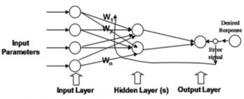
Neural networks contain units which are organized into input, hidden and output layers as shown in Figure 5. Shallow networks contain one hidden layer, the nodes within each layer are linked to nodes in neighboring layers. The computations in steps 1 and 2 occur for all neurons in the neural network, we talk about forward propagation. The results of forward propagation are compared, by the output layer, to the truth labels and adjust the weights if they have difference between results (predicted values) and truth labels. This process is called backpropagation, and the basics of this process can be summarized in 5 steps: (1) the neural network tries to reduce an objective function. (2) the network takes the derivative of total error, i.e., difference between predicted values and actual. This derivative is named gradient of the layer. (3) based on the gradient obtained in step 2, the weights are updated using the same gradient or a factor of it (called learning rate). (4) the process is repeated for each layer (5) values of gradients from previous layer can be used in next layer to make the gradient computation more efficient.
Figure 5. Neural network architecture
Noted that after one pass forward propagation and backpropagation the network layer’s weight is changed. The Gradient minimizes the overall error, so parameters number are converging to a low value and this convergence is named gradient descent.
Deep neural networks contain several hidden layers. Deep learning can be applied to various problems like classification, NLP, pattern recognition, predictive analysis, etc. Deep learning outperforms its predecessors.
The first model of deep learning was introduced in 1943 is the McCulloch-Pitts [17]. Based on the neural networks, the first computer model was created to mimic the neocortex of human brain [18]. The theory of Hebbian, employed in biological systems, was introduced [19] after the MCP model. After that, Frank Rosenblatt was created the “perceptron” the first electronic device in 1957 [19] based on MCP neuron. There are two types of perceptron’s:
·Perceptron with single layer which can only works with linear separation of data points (linearly separable patterns).
·Multilayer perceptron or know as feed forward neural network which contain two or more layers with more processing power.
In 1969, researchers indicate that neural networks couldn’t learn a basic XOR function [20], this phase know as AI-winter which AI didn’t get more interest and funding. At the end of AI winter, a backpropagation algorithm was introduced in 1970 [21] by Werbos. Backpropagation learning algorithms uses errors for training deep learning models, this technique was applied to neural networks in 1980. The difference between DNNs (deep neural networks) and earlier generation of machine learning techniques is the Automated feature extraction. In 1980 Kunihiko proposed the “neocognitron” [22] a hierarchical and multilayered neural network which inspired the convolutional neural networks, this network has been used for Japanese handwritten character recognition. In 1986, the Recurrent neural networks (RNN) were proposed. In 1990, LeNet [23] is the earliest convolutional neural networks which is trained and used to identify the handwritten digits in MNIST data set. In 2006, Deep Belief Network (DBN) was proposed by Hinton [24]. DBN is a deep generative network composed of several layers of stochastic latent variables, DBN is based on reinforcement learning and contains a stacked layer of RBM (Restricted Boltzmann Machine).
In contrast with shallow learning model (which contain few processing layers), deep learning contains deeper number of processing layers. Shallow architectures can’t be used for non-linear and complex functions.
Neural Network:
Often referred to as an artificial neural network (ANN), inspired from the structure of the human brain is a computational system. It is used for different tasks, such as regression and classification of data. Neural networks (NN) contain neurons organized in layers (input layer, one or more hidden layers, output layer).
Here's an overview of the key components and concepts related to NN:
1. Neurons (Nodes): Each neuron receives one or more inputs, processes them, and produces an output. Nodes are arranged into layers (input, output and one or more hidden layers).
2. Weights and Biases: Neurons apply weights to their inputs, and these weights determine the strength of the connections between neurons. In addition, each neuron has a bias term that can be adjusted to control its activation. Weight and bias values are learned during the training process.
3. Activation Function: is applied to the input weighted sum and biases to determine the neuron output; it can influence the network's learning capacity and behavior. Common activation functions include the sigmoid, ReLU (Rectified Linear Unit), and tanh functions.
4. Feedforward Propagation: In feedforward propagation, information travels through the network from the input to the output layer. In each layer, units apply the activation function to their inputs and pass the results to the next layer. This process generates predictions or outputs.
5. Loss Function: Measures the difference between the predicted output and the actual target values. The goal during training is to minimize this loss, typically using optimization techniques like gradient descent.
6. Backpropagation: updates the weights and biases in the network to minimize the loss. It involves calculating the loss gradients without modifying the model's parameters and adjusting those parameters in the direction that reduces the loss.
7. Hidden Layers: Neural networks can have one or more hidden layers. These layers contain neurons that capture and transform features from the input data. Deep neural networks, or deep learning models, have many hidden layers and are capable of learning complex patterns.
8. Training Data: Neural networks require labeled training data to learn the input and output relationships. The network learns from this data by adjusting its weights and biases during training.
9. Overfitting: Neural networks can be susceptible to overfitting, which signifies they might exhibit strong performance on the training data but poorly on unseen or new data. Methods like dropout, regularization, and cross-validation are used to mitigate overfitting.
10. Applications: Neural networks are used in image recognition, autonomous vehicles, and many more. Different network architectures and configurations are tailored to specific tasks.
Table 3. Examples of methods using NN to detect crop disease
|
Author |
Types of NN |
Diseases |
Accuracy |
|
Ferentinos et al. [14] |
VGG |
|
65.59% |
|
Lee et al. [25] |
CNN |
1269 tea disease images |
|
|
Amara et al. [26] |
LeNet |
three kinds of banana diseases |
99.71% |
|
Wang et al. [27] |
VGG16, VGG19, GoogLeNet and ResNet50 |
apple leaf black rot |
90.4% with VGG16 |
|
Fujita et al. [28] |
four-layer CNN |
cucumber diseases |
82.3% |
|
Abdulridha et al. [29] |
RBF, MLP |
Laurel wilt (Lw) disease |
98% |
|
Mohanty et al. [30] |
AlexNet and GoogleNet |
|
99.35% |
Neural networks are very popular in recent years, especially deep neural networks, due to their capability to learn intricate patterns and representations. They are at the core of many breakthroughs in artificial intelligence and have transformed industries such as healthcare, finance, and technology.
Table 3 illustrates the contributions of authors according to different Neural Networks for plant disease identification.
4.2 Proposed work
We propose a new technique to detect crop disease combining Autoencoder architecture and neural network. The idea is to compress all images using the Encoder; the output is called Latent space of autoencoder (or Bottleneck) which contains all unique features extracted by the Encoder. The Latent space represents data into low dimensional in vector form. We then used neural network architecture for classification; the input of this NN is the compressed data that we have got by our Encoder. After training, our algorithm achieves 90% accuracy which is a satisfactory outcome.
The entire tactic of crop disease classification is divided into three steps: after data processing, the Encoder extracts features, and we use neural network for classification.
4.2.1 Autoencoder for data compression
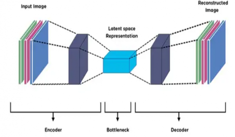
Autoencoder can extract a compressed representation of an input. It’s used for dimensionality reduction which is an approach to filter just the essential features of our crop data. Autoencoder is an unsupervised neural network used for automatic feature extraction from data. The autoencoder architecture is illustrated in the Figure 6.
Figure 6. Autoencoder architecture
We have three parts of autoencoder: Encoder, Latent space (Bottleneck) and Decoder. The encoder extracts essential feature from data and Decoder attempt to rebuild the original data based on compressed data in latent space vector. The output of autoencoder is the same as input with some loss.
In this paper we use just the first part of Autoencoder: Encoder and Latent space representation, the output is then reshaped to be inputted into neural network. Our novel proposed method has not been introduced in any previous research study.
The experiment demonstrates that Neural Network is the most effective classifier compared with other algorithms like CNN [31].
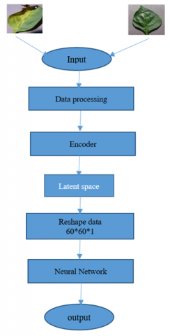
The architecture of our approach is illustrated in the Figure 7 below:
Figure 7. Overview of our proposed method
4.2.2 Neural network for classification
The Encoder compress data into latent space vector that contains all unique features from input data, we use then the NN as classifier. The training steps is illustrated in Figure 8 below:
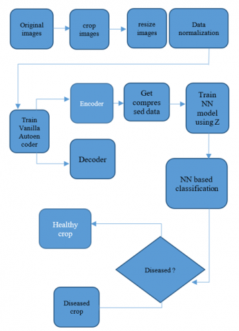
Figure 9 illustrates all steps of the proposed model.
We have three steps in the process of creating our novel model: the first step is to process data; we crop and resize images with size of 62*62 pixels. Resizing images can significantly speed up the model training. Then Vanilla autoencoder is created to minimize the dimensionality of data from 256*256 to 32*32, so we get the compressed data. Our autoencoder has three layers, we have used Adam optimizer and MSE function. Figure 10 illustrates the architecture of Vanilla autoencoder.
Figure 8. Training sequence of neural network classifier
Figure 9. Flowchart to explain our novel method
Figure 10. Architecture of Vanilla autoencoder
Table 4. Parameters used in NN
|
|
Neurons |
Input_Dimensions |
Weight Initializer |
Function |
|
Layer number 1 |
10 |
8 |
Uniform |
Rectified linear unit |
|
Layer number 2 |
6 |
- |
Uniform |
Rectified linear unit |
|
Layer number 3 |
1 |
|
Uniform |
sigmoid |
In this paper, we don’t use the Decoder of our autoencoder which try reconstructing the original. The loss function is mean squared error (MSE). The MSE formula is illustrated in Eq. (7):
$M S E=\frac{1}{n} \sum_{i=1}^n\left(y_{i-} \widetilde{y}_l\right)^2$ (7)
where, $y$ is the input crop image and $\tilde{y}$ represent the reconstructed image, while $n$ is the number of crops images.
After the operation of dimensionality reduction made by Vanilla autoencoder, the result of the Bottleneck layer serves as the input of our Neural Network classifier.
Table 4 above illustrates all parameters used in a NN.
4.3 PlantVillage dataset
In this paper, the dataset used is PlantVillage. We trained our model for three types of crops: Potato, Pepper, and Tomato and 8 types of crop diseases. Figure 11 illustrates examples of PlantVillage crop images:
We extracted crop images from 10 folders of PlantVillage dataset, the image size after extraction is 12080 and the extracted labels was: ['Pepper-bell-Bacterial-spot', 'Pepper-bell-healthy', 'Potato-Early-blight', 'Potato-Late-blight', 'Potato-healthy', 'Tomato-Bacterial-spot', 'Tomato-Early-blight', 'Tomato-Target-Spot', 'Tomato-Yellow-Leaf-Curl- Virus', 'Tomato_mosaic_virus']. The shape of our data is 12080*60*60*3 and 12080*10 for labels. 80% of the data is used for training the model, while the remaining 20% is reserved for testing. Thus, we have 9664 crop images for training dataset and 2416 crop images for testing dataset.
Figure 11. Images from PlantVillage dataset
4.4 Platform requirement
In this paper we used Jupyter Notebook, TensorFlow and Python version 3.8. The operating system used is windows 10 64 bits with a graphic card NVIDIA GEFORCE GTX and a RAM capacity of 12 GO. We also used a Core i7 processor.
The optimizer used for Vanilla autoencoder is Adam [32] and the loss function is MSE, we trained this algorithm with batch size of 32 and only seven epochs. We trained Neural network using binary cross-entropy (BCE) and Adam optimizer with five epochs and batch size of 32.
The choice of the Adam optimizer algorithm for training neural networks is a common and popular one for several compelling reasons:
1. Adaptive Learning Rates: Adam, which stands for "Adaptive Moment Estimation," adjusts the learning rate during training for each parameter individually. This adaptability is crucial because it helps the model converge faster and more reliably. It dynamically scales the learning rates based on the gradients of each parameter, ensuring that small and large updates are made appropriately. Adam utilizes estimations of both the first and second moments of the gradient to adjust the weight learning rate dynamically. For a random variable, the moment is calculated as follow:
$m_n=E\left[X^n\right]$ (8)
m: moment, X: random variable.
2. Momentum and RMSprop Combination: Momentum helps the optimizer navigate through flat regions and accelerates convergence, while RMSprop helps control the learning rates for each parameter based on the magnitude of recent gradients. The combination of these two techniques often results in faster convergence and better optimization.
3. Low Memory Requirements: Adam maintains exponentially moving averages of the gradients and squared gradients, which requires relatively low memory compared to some other optimization algorithms. This is advantageous when dealing with large models or when training on hardware with limited memory. To calculate the moments, Adam uses exponentially moving averages based on the gradients calculated from the current mini batch:
$m_t=\beta_1 m_{t-1}+\left(1-\beta_1\right) g_t$ (9)
$v_t=\beta_2 v_{t-1}+\left(1-\beta_2\right) g_t^2$ (10)
m and v: moving averages.
g: the gradient.
4. Consistent Performance: While no optimizer is universally the best for every problem, Adam tends to provide consistently good performance across a variety of tasks. It has become a good choice in the deep learning community.
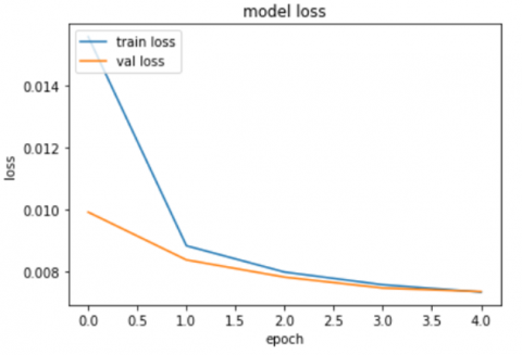
The first operation in our method is data processing, which we crop and resize all dataset images. Then we feed the new dataset in our autoencoder to compress data. After only 5 epochs, the loss of autoencoder reached 73 10-4; Figure 12 below shows the loss of our Encoder, while Figure 13 illustrates an overview of compressed data.
Figure 12. Training loss and validation loss for vanilla autoencoder
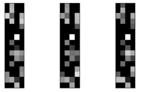
The overview of the compressed images is show in Figure 13:
Figure 13. Compressed images by the encoder
Visualize latent space data:
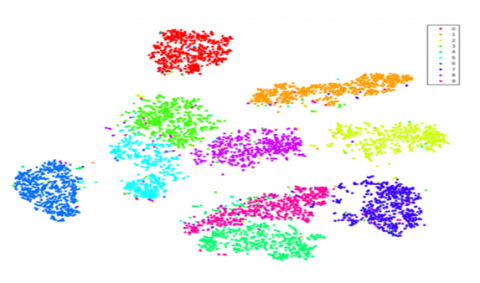
To visualize latent space data, we can use T-SNE technique to project our data into autoencoder Latent space. Figure 14 below shows the projection of our data into Latent space of autoencoder:
Figure 14. Projection of data into latent space
T-SNE is a technique for dimensionality reduction employed in machine learning and data visualization. It's particularly useful for visualizing data in a lower-dimensional space without losing important data.
Here's how T-SNE works:
1. High-Dimensional Input Data: t-SNE takes as input a dataset with a high number of dimensions, such as data points with many features.
2. Pairwise Similarities: It begins by computing pairwise similarities between data points. Typically, t-SNE uses the Gaussian distribution to measure the similarity between points, with closer points having higher similarities.
3. Probabilities: These similarities are used to create probability distributions over pairs of points. In the high-dimensional space, the probability is based on the similarities computed in step 2.
4. Minimizing Divergences: The T-SNE objective is to find a mapping that minimizes the divergence between these two probability distributions. This is achieved, in low-dimensional space, using an optimization process that adjusts the positions of the points.
5. Gradient Descent: is used in the low-dimensional space to minimize the divergence between the two probability distributions by adjusting the positions of the points.
6. Preservation of Structure: The optimization process continues until the low-dimensional representation aligns well with the high-dimensional data, saving the relationships and the structure of data.
One key characteristic of t-SNE is that it tends to group similar data points closely together in the low-dimensional space, which makes it excellent for visualizing clusters or patterns in the data. However, it's important to note that t-SNE is not suitable for dimensionality reduction for other machine learning tasks; it's primarily used for visualization.
Figure 15 below depicts the application of T-SNE on the MNIST dataset. The MNIST dataset is known for containing images of handwritten digits, making it a popular choice for tasks such as digit classification. T-SNE is used as a technique to visualize and cluster the data points within this dataset, providing insights into the distribution and relationships between different handwritten digits. Figure 15 illustrates T-SNE on mnist dataset.
In summary, T-SNE is a powerful tool for visualizing data by projecting it into a lower-dimensional area while preserving the underlying structure and relationships, making it a valuable technique for exploratory data analysis and pattern recognition.
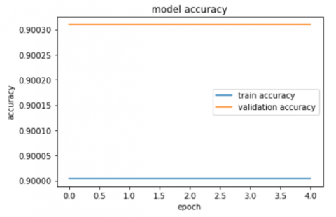
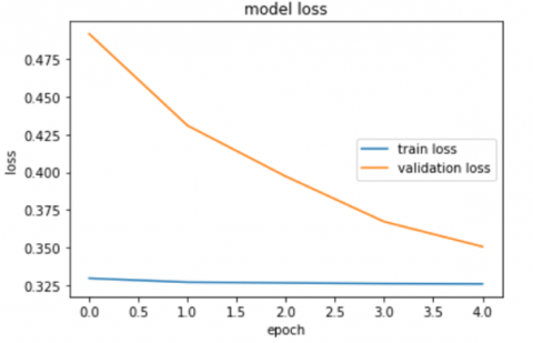
The second step of our method is to build neural network for binary classification. The Encoder output is the input of the neural network with three layers. After five epochs our model reached 90% and 89% for training and validation accuracy respectively. Figure 16 and Figure 17 illustrates the accuracy and the loss of our classifier respectively.
Figure 15. Illustration of T-SNE on mnist dataset
Figure 16. Training and validation accuracy
Figure 17. Representation of the neural network loss
Based on training time, we will compare our method with state-of-the-art methods such as CNN, Resnet152, and VGG19. As we can see in Table 5, our proposed method outperforms all other method and has training time less than 95 second unlike all compared methods.
Table 5. Benchmarks based on training time
|
Methods |
Training Time (per second) |
Number of Epochs |
Batch Size |
|
Neural network model |
22.014 |
5 |
30 |
|
Autoencoder model |
30.81 |
7 |
30 |
|
The proposed method |
52.824 |
- |
30 |
|
CNN [33] |
159.14 |
7 |
30 |
|
Resnet-152 [34] |
1281 (21 minutes20 seconds) |
7 |
30 |
|
VGG-19 [35] |
8.77 |
7 |
30 |
|
AlexNet [36] |
850 (14 minutes 10 seconds) |
7 |
30 |
|
GoogLeNet (Inception V1) [37] |
3716.42 (61.94 minutes) |
7 |
30 |
|
Inception V 3 [38] |
825.87 (14 minutes) |
7 |
30 |
|
VGG 16 [39] |
913.73 (15 minutes) |
7 |
30 |
|
DenseNet121 [40] |
791.99 (13 minutes) |
7 |
30 |
|
SqueezeNet [41] |
152.23 |
7 |
30 |
Table 5 illustrates the comparison of training time between state-of-the-art methods and the proposed work (batch size= 30, epochs = 7).
As we can see in Table 5above, the proposed method ALS-NN (Autoencoder Latent Space – Neural network) identifies crop disease in less time than other works, after only 22.014 second the classifier neural network (NN) can identify accurately crop disease after 5 epochs only while CNN and ResNet-152 exceeds 100 seconds. So, our novel method outperforms other works, and it is less time consuming.
The accuracy comparison is illustrated in Table 6. As illustrated, our proposed technique outperforms all these algorithms after only 5 epochs (batch size = 30, epochs = 7).
Table 6. Accuracy benchmark
|
Methods |
Accuracy |
Loss |
|
The proposed model |
0.90 |
0.3252 |
|
Resnet-152 |
0.89 |
0.32 |
|
AlexNet |
0.90 |
0.0000e+00 |
|
GoogleNet (Inception V1) |
0.90 |
Nan |
|
Inception V 3 |
0.895 |
0.2988 |
|
VGG 16 |
0.9651 |
0.0890 |
|
DenseNet121 |
0.90 |
0.0000e+00 |
|
SqueezeNet |
0.2078 |
2.13 |
|
CNN |
0.87 |
0.2838 |
|
VGG-19 |
0.10 |
0.0000e+00 |
As illustrated in Table 6, the proposed method achieved 90% testing accuracy which is more than Resnet-152, VGG and CNN (with three layers). The validation accuracy of ALS-NN method is 90% which is a good accuracy compared with other techniques like VGG19 with validation accuracy 10%, and ResNet-152 with validation accuracy 90%, and CNN with validation accuracy 86% but after 7 epochs.
On the other hand, ALS-NN is trained using less parameters compared with VGG, Resnet159 and CNN networks. Table 7 below shows a comparative study of our methods and other techniques based on a number of trainable parameters.
As illustrated in Table 7, our method is trained with less parameters compared with VGG, Resnet-152 and CNN with less than 90 000 parameters for Vanilla autoencoder and only 163 parameters for NN classifier. To reach the same accuracy as our method, Resnet-152 needs more than 8 million trained parameters, so the proposed system outperformed the state-of-the-art systems based on trained parameters.
Significance of Results:
Our proposed model can be used in the agriculture area to speed up the process of crop disease identification which can increase crop yield by identifying and addressing crop disease promptly. So, farmers maintain healthier crops leading to increased yield. This is vital for food production to address the needs of an expanding global population. Our model can enable precise and targeted treatment by identifying diseases timely which can significantly reduce the need for chemical pesticides and fungicides, leading to cost savings for farmers and decreased environmental impact.
The use of ALS-NN can improve resource management with accurate disease identification, so farmers can allocate resources more efficiently. They can focus on the areas of their fields that need attention, saving time and resources. By reducing crop losses and optimizing resource use, our model ALS-NN can lead to cost savings for farmers. This is especially crucial for small-scale farmers and those in developing regions like Morocco. Our model is a good tool for farmers to tackle disease outbreaks effectively, maximize crop yields, and contribute to global food security.
Table 7. Benchmark based on number of trainable parameters between ALS-NN and other works
|
Method |
Number of Trainable Parameters |
Testing Accuracy |
Validation Accuracy |
|
CNN |
2,685,898 |
87% |
86% |
|
ALS-NN (our method) |
Autoencoder: 87,139 NN classifier: 163 |
90% |
90% |
|
VGG 19 |
263,169 |
10.01% |
10% |
|
Resnet-152 |
8,203,010 |
89.99% |
90% |
|
AlexNet |
28,846,051 |
90% |
90% |
|
GoogLeNet (Inception V1) |
|
90% |
90% |
|
Inception V 3 |
40,644,769 |
89.5% |
90% |
|
VGG 16 |
14,714,688 |
96.51% |
- |
|
DenseNet121 |
6,954,881 |
90% |
90% |
|
SqueezeNet |
727,632 |
20.78% |
21.98% |
The Internet of things plays a significant role in smart agriculture; IoT sensors can provide more information about crops which can positively affect crop production by monitoring environmental factors. Using IoT we can expect an increase of production with low cost by monitoring temperature, humidity, fertilizer, and soil efficiency.
Certainly, IoT has played a crucial role in smart agriculture, enabling farmers to monitor and manage their operations more efficiently. Here are some specific examples of how IoT has been used in agriculture and the impact it has had:
1. Precision Agriculture: IoT sensors are used for data collection (temperature or soil moisture…). This data helps farmers to take precise decisions about irrigation and fertilization.
2. Weather and Environmental Monitoring: Collect data like precipitation, humidity, and temperature. This information is vital for optimizing planting, irrigation management, and mitigating weather-related risks.
3. Crop Health Monitoring: using drones with cameras and IoT sensors. The data and captured images are analyzed to identify signs of disease.
4. Automated Irrigation: the system of irrigation is controlled based on IoT. This prevents over-irrigation, conserves water, and reduces energy costs.
5. Supply Chain Management: IoT helps in tracking the movement of crops and produce from farm to market. Sensors on storage containers monitor temperature and humidity to ensure perishable goods safety.
6. Livestock Feed Management: Smart feeders use IoT technology to dispense the right amount of feed for animals, reducing waste and ensuring optimal nutrition.
7. Farm Equipment Maintenance: IoT sensors on tractors and other farming machinery monitor performance and send alerts when maintenance is needed. This proactive approach reduces downtime and improves operational efficiency.
8. Labor Efficiency: IoT can help with labor management by tracking worker activity and optimizing work schedules and assignments.
The impact of IoT in agriculture has been substantial:
·Increased Productivity: IoT enables data-driven decision-making, resulting in higher crop yields, healthier livestock, and more efficient resource use.
·Resource Conservation: IoT helps reduce water and energy consumption by optimizing irrigation, reducing wastage, and promoting sustainable practices.
·Cost Reduction: By improving efficiency, IoT lowers operational costs, making farming more profitable.
·Sustainability: IoT supports sustainable agriculture by minimizing the environmental impact of farming practices.
·Improved Quality and Safety of agricultural products.
·Risk Mitigation: Early disease detection and weather monitoring allow farmers to take proactive measures, reducing crop and livestock losses.
In summary, IoT has revolutionized agriculture by giving farmers real-time information and control over various aspects of their operations. The impact is evident in increased productivity, resource efficiency, cost reduction, and overall sustainability.
In this paper we can monitor temperature and humidity in agriculture field through sensors using Raspberry Pi 3 model B+. The camera is connected to Raspberry Pi to capture crop images and use our proposed algorithm ALS-NN to identify crop diseases.
7.1 Concept of IoT
Internet of things (IoT) describes a system where the world is connected to Internet using several sensors. IoT is a vision where all objects (vehicles, furniture, roads, etc..) are controllable, locatable, and recognizable via the Internet.
Using IoT can improve accuracy, efficiency and economic benefit and reduce human intervention [42].
7.1.1 Raspberry Pi
The Raspberry Pi is a compact single-board computer used for small networking operations and computing. It’s one of the important elements in the field of IoT. Using the Internet, Raspberry Pi can connect remote location controlling devices with automation system. In this paper we used Raspberry Pi version 3 B+, it has quad-core has quad-core ARM Cortex-A53 CPU of 900 MHz, and 1GB LPDDR2 SDRAM. It has 4 usb ports, Ethernet port, HDMI port, video camera interface, display interface DCI, and SD card slot. Here are some reasons why the Raspberry Pi 3 Model B+ might be chosen over other options:
·Performance: It offers a significant boost in performance compared to its predecessors.
·Built-in Wireless Connectivity: The Model B+ comes with built-in dual-band Wi-Fi (2.4GHz and 5GHz) and Bluetooth 4.2. This integrated wireless connectivity simplifies connectivity and communication, which is important for many IoT and networked projects.
·Availability and Community Support: The Raspberry Pi 3 Model B+ benefits from a large and active user community, ensuring easy access to tutorials, documentation, and community support. The availability of resources and expertise is a major advantage for both beginners and experienced users.
·Cost-Efficiency: Raspberry Pi boards are known for their cost-effectiveness. The Model B+ offers a good balance of performance and features for its price, making it an attractive choice for projects with budget constraints.
·Compatibility: The Model B+ maintains compatibility with many of the existing Raspberry Pi accessories, including cases, power supplies, and HATs (Hardware Attached on Top). This can save time and money when transitioning from a previous Raspberry Pi model.
·GPIO Pins: It comes with a 40-pin GPIO header, which is important for hardware and DIY projects that require interfacing with sensors, motors, and other external components.
·Energy Efficiency: It is relatively energy-efficient, consuming only a modest amount of power. This can be important for projects where power consumption is a consideration.
·Operating System Support: The Model B+ enjoys wide operating system support, including various flavors of Linux and even Windows 10 IoT Core, making it versatile and compatible with a variety of software applications.
7.1.2 Temperature sensor
DS18B20 temperature sensor is used to measure temperature. Waterproof probe based on a DS18B20 allowing temperature measurement from -55 to +125°C. It is connected to a microcontroller via digital input.
7.1.3 Humidity sensor
This sensor measures the water content in soil and transfers it to Raspberry Pi (our microcontroller) to act of switching water pump on/off.
7.1.4 Power supply
Raspberry Pi 12.5W Micro USB Power Supply with 5.1V / 2.5A DC output.
7.1.5 Camera Raspberry Pi
A 5MP (5 Megapixels) camera for Raspberry Pi. Easy to install, an ideal solution for designing a Webcam, IP Camera, or CCTV Camera from the Raspberry Pi. It has a number of pixels 2592*1944 with sensor size of 3.67*2.74 mm.
Temperature, humidity, and camera sensors are commonly chosen for agricultural monitoring systems because they provide critical data that can significantly impact crop and livestock management. Here's why these specific sensors are commonly used:
1. Temperature Sensors:
·Crop Health: Temperature affects plant growth and development. Monitoring temperature helps farmers assess the suitability of their environment for specific crops. Different crops have specific temperature requirements for optimal growth.
·Frost and Freeze Protection: Monitoring temperature is essential to protect crops from frost and freezing temperatures. When temperatures drop below critical levels, automated systems can activate heaters or fans to safeguard crops.
·Energy Efficiency: Temperature data allows for the efficient use of heating and cooling systems. This reduces energy consumption and lowers operational costs.
2. Humidity Sensors:
·Irrigation Management: Humidity levels are closely related to the need for irrigation. Monitoring humidity helps in determining when and how much to irrigate. It prevents over- or under-watering, promoting healthy crop growth.
·Disease Prevention: Certain plant diseases thrive in humid conditions. Monitoring humidity can help in disease prediction and management. Farmers can take preventive measures when humidity levels are conducive to disease development.
·Storage and Preservation: In post-harvest storage, humidity control is crucial to prevent spoilage and maintain the quality of agricultural products. Sensors help maintain the optimal storage environment.
3. Camera Sensors:
·Crop Health Assessment: Cameras capture images of crops, allowing for visual assessment of their health and growth. ALS-NN models can be used to analyze images for crop disease identification.
·Pest and Weed Detection: Cameras can detect the presence of pests and weeds, enabling farmers to take timely action. This reduces the need for chemical treatments and minimizes crop damage.
·Quality Control: Cameras in packing and processing facilities help in quality control by ensuring that agricultural products meet the desired standards. They can detect defects and sort produce accordingly.
·Research and Data Collection: Images collected from cameras can be valuable for research and historical data analysis. They provide a visual record of the development and health of crops over time.
These sensors are chosen to produce real-time information that is critical for decision-making in agriculture. By monitoring temperature, humidity, and using cameras for visual data, farmers can improve crop management, minimize risks, and optimize resource usage. These sensors are integral to the shift towards data-driven precision agriculture, where decisions are made based on accurate and timely information, ultimately leading to better yields and sustainability in farming.
7.2 Proposed system model
To monitor crop healthiness, we used an intelligent system with various sensors which can collect information from the fields accurately. The camera connected to Raspberry Pi takes pictures of crops and sends them to our proposed system ALS-NN to identify crop disease.
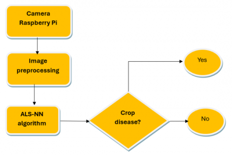
Figure 18 below illustrate how we can identify crop disease with camera of Raspberry Pi and our system:
Figure 18. Using camera Raspberry Pi and our proposed method to identify crop disease
The Raspberry Pi microcontroller is the core component of this system. It controls the working of each device connected to it. The important device connected to Raspberry Pi is camera with 5 Megapixels:
(1) A camera is fitted which will capture pictures of the crop.
(2) This image is sent to our system to be analyzed.
(3) After image processing, we used our proposed algorithm ALS-NN to identify crop disease.
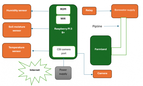
Figure 19. Blog diagram for smart agriculture
Figure 19 illustrates the block diagram of proposed system model.
Crop disease identification is a challenging task, much research used deep learning and neural network to identify crop diseases. However, the downside of these methods is that they are time consuming and trained with millions of parameters which need performed computer. To address these issues, the proposed method ALS-NN used two networks, the first network is Vanilla autoencoder and Neural Network (NN). The first network compress data using the Encoder and feeds this output to the second network for classification. The autoencoder reduces extracted features number, without losing the important features, which also reduces the training time of our system which is the main contribution of this paper. The ALS-NN model works by compressing the data to utilize only the most critical information during the classification process. Vanilla Autoencoder is used for data compression by using the Encoder which is the first half of Autoencoder. The encoder takes high dimensional input data and transforms it into lower-dimensional representation without losing the important information. The encoder ultimately compresses data, and the result is called bottleneck, which represents a compact and informative representation of the original data. The compressed data is classified using neural network. This compression significantly speeds up the model and reduces the parameters number which outperform the state-of-the-art model. By combining Autoencoder and Neural Network [43] technologies effectively, we achieve a fast model with fewer parameters. As a result, disease detection operations are much quicker, which helps mitigate the negative impact of these plant diseases on crop yields.
Our system attained a testing accuracy of 90% and a validation accuracy of 90%. This system uses a few numbers of trained parameters (163 for Neural Network, 87139 for autoencoder). The implementation of the ALS-NN model can enhance resource management through precise disease identification. This allows farmers to allocate their resources more efficiently, as they can concentrate their efforts on the specific field’s areas. This not only saves time but also conserves valuable resources, resulting in more effective and sustainable farming practices.
[1] Nandhini, S., Ashokkumar, K. (2022). An automatic plant leaf disease identification using DenseNet-121 architecture with a mutation-based henry gas solubility optimization algorithm. Neural Computing and Applications, 34: 5513–5534. https://doi.org/10.1007/s00521-021-06714-z
[2] Shadin, N.S., Sanjana, S., Lisa, N.J. (2021). COVID-19 diagnosis from chest X-ray images using convolutional neural network (CNN) and InceptionV3. In 2021 International Conference on Information Technology (ICIT), Amman, Jordan, pp. 799-804. https://doi.org/10.1109/ICIT52682.2021.9491752
[3] Khan, E., Rehman, M.Z.U., Ahmed, F., Khan, M.A. (2021). Classification of diseases in citrus fruits using SqueezeNet. In 2021 International Conference on Applied and Engineering Mathematics (ICAEM), Taxila, Pakistan, pp. 67-72. https://doi.org/10.1109/ICAEM53552.2021.9547133
[4] Bharathi, I., Sonai, V. (2022). Image-based crop leaf disease identification using convolution encoder networks. In Machine Learning and Data Mining-Annual. https://doi.org/10.5772/intechopen.106989
[5] Khamparia, A., Saini, G., Gupta, D., Khanna, A., Tiwari, S., de Albuquerque, V.H.C. (2020). Seasonal crops disease prediction and classification using deep convolutional encoder network. Circuits, Systems, and Signal Processing, 39: 818-836. https://doi.org/10.1007/s00034-019-01041-0
[6] Sanga, S., Mero, V., Machuve, D., Mwanganda, D. (2020). Mobile-based deep learning models for banana diseases detection. arXiv preprint arXiv:2004.03718. https://arxiv.org/abs/2004.03718
[7] Chohan, M., Khan, A., Chohan, R., Katpar, S.H., Mahar, M.S. (2020). Plant disease detection using deep learning. International Journal of Recent Technology and Engineering, 9(1): 909-914. https://doi.org/10.35940/ijrte.A2139.059120
[8] Mohameth, F., Bingcai, C., Sada, K.A. (2020). Plant disease detection with deep learning and feature extraction using plant village. Journal of Computer and Communications, 8(6): 10-22. https://doi.org/10.4236/jcc.2020.86002
[9] Tiwari, D., Ashish, M., Gangwar, N., Sharma, A., Patel, S., Bhardwaj, S. (2020). Potato leaf diseases detection using deep learning. In 2020 4th International Conference on Intelligent Computing and Control Systems (ICICCS), Madurai, India, pp. 461-466. https://doi.org/10.1109/ICICCS48265.2020.9121067
[10] Sibiya, M., Sumbwanyambe, M. (2019). A computational procedure for the recognition and classification of maize leaf diseases out of healthy leaves using convolutional neural networks. AgriEngineering, 1(1): 119-131. https://doi.org/10.3390/agriengineering1010009
[11] Türkoğlu, M., Hanbay, D. (2019). Plant disease and pest detection using deep learning-based features. Turkish Journal of Electrical Engineering and Computer Sciences, 27(3): 1636-1651. https://doi.org/10.3906/elk-1809-181
[12] Too, E.C., Yujian, L., Njuki, S., Yingchun, L. (2019). A comparative study of fine-tuning deep learning models for plant disease identification. Computers and Electronics in Agriculture, 161: 272-279. https://doi.org/10.1016/j.compag.2018.03.032
[13] Pardede, H.F., Suryawati, E., Sustika, R., Zilvan, V. (2018). Unsupervised convolutional autoencoder-based feature learning for automatic detection of plant diseases. In 2018 International Conference on Computer, Control, Informatics and its Applications (IC3INA), Tangerang, Indonesia, pp. 158-162. https://doi.org/10.1109/IC3INA.2018.8629518
[14] Ferentinos, K.P. (2018). Deep learning models for plant disease detection and diagnosis. Computers and Electronics in Agriculture, 145: 311-318. https://doi.org/10.1016/j.compag.2018.01.009.
[15] Napte, K., Mahajan, A. (2022). Deep learning based liver segmentation: A review. Revue d'Intelligence Artificielle, 36(6): 979-984. https://doi.org/10.18280/ria.360620
[16] LeCun, Y., Bengio, Y., Hinton, G. (2015). Deep learning. Nature, 521: 436–444. https://doi.org/10.1038/nature14539
[17] McCulloch, W.S., Pitts, W. (1943). A logical calculus of the ideas immanent in nervous activity. Bulletin of Mathematical Biophysics 5, 4: 115-133.
[18] Schmidhuber, J. (2015). Deep learning in neural networks: An overview. Neural Networks, 61: 85-117. https://doi.org/10.1016/j.neunet.2014.09.003.
[19] Rosenblatt, F. (1958). The perceptron: A probabilistic model for information storage and organization in the brain. Psychological Review, 65(6): 386-408. https://psycnet.apa.org/doi/10.1037/h0042519.
[20] Minsky, M., Papert, S.A. (1969). Perceptrons: An introduction to computational geometry, expanded edition. Cambridge, MA, USA: MIT Press, p. 258.
[21] Werbos, P. (1974). Beyond regression: New tools for prediction and analysis in the behavioral sciences. PhD thesis, Committee on Applied Mathematics, Harvard University, Cambridge, MA.
[22] Fukushima, K. (1980). Neocognitron: A self-organizing neural network model for a mechanism of pattern recognition unaffected by shift in position. Biological Cybernetics, 36(4): 193-202. https://doi.org/10.1007/BF00344251.
[23] Yu, N., Jiao, P., Zheng, Y. (2015). Handwritten digits recognition base on improved LeNet5. In the 27th Chinese Control and Decision Conference (2015 CCDC), pp. 4871-4875. https://doi.org/10.1109/CCDC.2015.7162796.
[24] Hinton, G.E. (2009). Deep belief networks. Scholarpedia, 4(5): 5947.
[25] Lee, S.H., Wu, C.C., Chen, S.F. (2018). Development of image recognition and classification algorithm for tea leaf diseases using convolutional neural network. In 2018 ASABE Annual International Meeting (p. 1). American Society of Agricultural and Biological Engineers. https://doi.org/10.13031/aim.201801254
[26] Amara, J., Bouaziz, B., Algergawy, A. (2017). A deep learning-based approach for banana leaf diseases classification. Datenbanksysteme für Business, Technologie und Web (BTW 2017)-Workshopband.
[27] Wang, G., Sun, Y., Wang, J. (2017). Automatic image-based plant disease severity estimation using deep learning. Computational Intelligence and Neuroscience, 2017: 2917536. https://doi.org/10.1155/2017/2917536
[28] Fujita, E., Kawasaki, Y., Uga, H., Kagiwada, S., Iyatomi, H. (2016). Basic investigation on a robust and practical plant diagnostic system. In 2016 15th IEEE International Conference on Machine Learning and Applications (ICMLA), pp. 989-992. https://doi.org/10.1109/ICMLA.2016.0178
[29] Abdulridha, J., Ehsani, R., De Castro, A. (2016). Detection and differentiation between laurel wilt disease, phytophthora disease, and salinity damage using a hyperspectral sensing technique. Agriculture, 6(4): 56. https://doi.org/10.3390/agriculture6040056
[30] Mohanty, S.P., Hughes, D.P., Salathé, M. (2016). Using deep learning for image-based plant disease detection. Frontiers in Plant Science, 7: 1419. https://doi.org/10.3389/fpls.2016.01419
[31] Patil, A., Rane, M. (2021). Convolutional neural networks: an overview and its applications in pattern recognition. Information and Communication Technology for Intelligent Systems: Proceedings of ICTIS 2020, 1: 21-30. https://doi.org/10.1007/978-981-15-7078-0_3
[32] Kingma, D.P., Ba, J. (2014). Adam: A method for stochastic optimization. arXiv preprint arXiv:1412.6980. https://arxiv.org/abs/1412.6980.
[33] Soufi, O., Belouadha, F.Z. (2022). Study of deep learning-based models for single image super-resolution. Revue d'Intelligence Artificielle, 36(6): 939-952. https://doi.org/10.18280/ria.360616
[34] Shafiq, M., Gu, Z. (2022). Deep residual learning for image recognition: A survey. Applied Sciences, 12(18): 8972. https://doi.org/10.3390/app12188972
[35] Nguyen, T.H., Nguyen, T.N., Ngo, B.V. (2022). A VGG-19 model with transfer learning and image segmentation for classification of tomato leaf disease. AgriEngineering, 4(4): 871-887. https://doi.org/10.3390/agriengineering4040056
[36] Chen, H.C., Widodo, A.M., Wisnujati, A., Rahaman, M., Lin, J.C.W., Chen, L., Weng, C. E. (2022). AlexNet convolutional neural network for disease detection and classification of tomato leaf. Electronics, 11(6): 951. https://doi.org/10.3390/electronics11060951
[37] Sharma, S., Kumar, H. (2022). Detection and classification of plant diseases by Alexnet and GoogleNet deep learning architecture. International Journal of Scientific Research & Engineering Trends, 8(1): 218-223.
[38] Jenipher, V.N., Radhika, S. (2022). An automated system for detecting rice crop disease using CNN inception V3 transfer learning algorithm. In 2022 Second International Conference on Artificial Intelligence and Smart Energy (ICAIS), Coimbatore, India, pp. 88-94. https://doi.org/10.1109/ICAIS53314.2022.9742999
[39] Thakur, P.S., Sheorey, T., Ojha, A. (2023). VGG-ICNN: A lightweight CNN model for crop disease identification. Multimedia Tools and Applications, 82(1): 497-520. https://doi.org/10.1007/s11042-022-13144-z
[40] Dubey, N., Bhagat, E., Rana, S., Pathak, K. (2022). A novel approach to detect plant disease using DenseNet-121 neural network. In Smart Trends in Computing and Communications: Proceedings of SmartCom 2022, pp. 63-74. https://doi.org/10.1007/978-981-16-9967-2_7
[41] Setiawan, W., Ghofur, A., Rachman, F.H., Rulaningtyas, R. (2021). Deep convolutional neural network alexnet and squeezenet for maize leaf diseases image classification. Kinetik: Game Technology, Information System, Computer Network, Computing, Electronics, and Control. https://doi.org/10.22219/kinetik.v6i4.1335
[42] Szegedy, C., Liu, W., Jia, Y., Sermanet, P., Reed, S., Anguelov, D., Erhan, D., Vanhoucke, V., Rabinovich, A. (2015). Going deeper with convolutions. In Proceedings of the IEEE Conference on Computer Vision and Pattern Recognition, Boston, MA, USA, pp. 1-9. https://doi.org/10.1109/CVPR.2015.7298594
[43] Lachouri, C.E., Mansouri, K., Lafifi, M.M. (2022). Greenhouse climate modeling using fuzzy neural network machine learning technique. Revue d'Intelligence Artificielle, 36(6): 925-930. https://doi.org/10.18280/ria.360614