Mudassar H. Naikwadi*![]() | Kishor P. Patil
| Kishor P. Patil![]()
© 2023 IIETA. This article is published by IIETA and is licensed under the CC BY 4.0 license (http://creativecommons.org/licenses/by/4.0/).
OPEN ACCESS
In wireless communications, cognitive radio (CR) technology has significantly enhanced radio spectrum efficiency. Spectrum sensing is a key process in CR along with other major functions namely spectrum decision, sharing and mobility. Minimizing the processing delays, energy consumption of these functions and enhancing spectrum utilization is a major challenge. Spectrum inference has been proposed as a viable solution to overcome these problems. Many machine learning-based spectrum inference techniques using artificial neural networks (ANNs) and deep neural networks have been proposed in literature. In this paper we aimed to determine whether hybrid deep neural network based spectrum inference model outperform single model in time and frequency domains for spectrum occupancy dataset. Radial basis function (RBF) neural network tend to excel in extracting spatial features of spectrum data whereas bidirectional long short-term memory (BiLSTM) work very well for temporal dependencies of this data. Spectrum dataset exhibit both short-and-long term temporal/spectral dependencies. In this paper we have proposed spectrum inference based on a hybrid deep neural network RBF and BiLSTM. The proposed algorithm has been simulated using real time spectrum measurement data with time dimension ranging from (1 to 7 days), spectral range (0.7 GHz to 2.7 GHz) across three geographically varying locations Pune, Solapur and Kalaburagi in India. Hybrid deep neural network integration of RBF and BiLSTM is built, tested and compared with single models LSTM, BiLSTM for accuracy and speed. The hybrid method has outperformed single models to achieve Precision, Recall, F1 scores of 0.9959, 0.9575, 0.9763 respectively and training time improvement of 57.60% for GSM and whole band in frequency and time dimensions.
artificial intelligence, cognitive radio networks, deep learning, deep neural networks, hybrid deep neural networks, machine learning, spectrum inference
Wireless communication is a vital means of communication. It uses radio spectrum which is a limited natural resource. Due to exponential growth in wireless services and applications spectrum has become scarce. Studies have also reported inefficient spectrum management due to static allocation policies. To overcome this dynamic spectrum access has been proposed as solution. Cognitive Radio (CR) is an enabling technology for dynamic spectrum access. It is an intelligent radio which efficiently manages spectrum between primary user and secondary users [1].
CRs exhibit four major functions spectrum sensing, spectrum decision, spectrum sharing and spectrum mobility [2]. Spectrum sensing is at the core of these four functions to determine unused vacant bands. However, the available spectrum sensing techniques hinder CR performance due to inevitable sensing time delays, high energy consumption and slow speed. To overcome these deficiencies spectrum inference has been proposed as novel technique to predict unused bands using historical spectrum occupancy data. It has become popular amongst researchers due to its pro activeness and widening of sensing scope in different bands across different locations [3].
Machine learning and deep learning algorithms based on artificial neural networks (ANN) are being employed for implementing spectrum inference in CRs. Multi Layer Perceptron (MLP), Radial Basis Function (RBF), Long Short Term Memory (LSTM) have been used for implementing spectrum inference. 6G CRNs major emphasis is on intelligence and spectrum inference compliments this approach. It is a realm where communication meets Artificial Intelligence (AI). Machine learning techniques applied to cognitive radios have been detailed by Bkassinyin et al. [4]. Arivudainambi et al. [5] have reported enhanced prediction accuracy and decrease in sensing time with spectrum inference using ML technique. Classical statistical occupancy prediction and ML based spectrum occupancy prediction has been detailed by Eltom et al. [6] Supervised and unsupervised ML algorithms for spectrum occupancy prediction have been analyzed by Azmat et al. [7].
Shrestha and Mahmood [8] have presented a comprehensive review of deep learning architectures, trainings, issues and implementations. Yu et al. [9] proposed spectrum prediction LSTM model validated by real-world spectrum dataset with taguchi method. Aygul et al. [10] has proposed composite 2D LSTM model for spectrum inference by harnessing correlations in the measured data. Siami-Namini et al. [11] has compared the performance and behavioral analysis of LSTM and BiLSTM and reported better predictions compared to LSTMs by almost 38% error rate reduction. A hybrid approach combining ANNs and deep neural networks has been employed in many fields. Hybrid approach has been employed by Fathi et al. [12] for stock price prediction. Riyaz et al. [13] has developed a deep neural network prediction model for heart disease with a novel ensemble technique. Kowsher et al. [14] deeply integrated BiLSTM-ANN and LSTM-ANN and reported performance improvements than single BiLSTM, LSTM and ANN models. Patil and Adhiya [15] have addressed automated evaluation of short descriptive answers using Siamese stacked BiLSTM model. Wang et al. [16] has proposed long short-term memory time forecasting with back propagation method and has reported 1% to 2% rise in prediction accuracy compared to LSTM.
In this study the dataset is a complex time series featuring different telecommunication bands and has both short as well as long term dependencies. RBFN networks have capability to model complex nonlinear data, in high dimensional data with good degree of accuracy. It also achieves fast inference with fast training as radial basis function simplifies computations. BiLSTM networks work well for data with complex dependencies over long intervals. It employs dual training for better extraction of context in data. Combining RBFN and BiLSTM can help model temporal, spectral dependencies and nonlinear patterns collectively in our dataset. Since RBFNs excel in meaningful extraction of features of complex data and BiLSTMs effectively capture context and dynamicity in dataset. Hence these advantages complement each other for a comprehensive learning and can deliver benefits of accurate fast prediction for spectrum dataset. So a hybrid model combining these two networks has been chosen for research in this paper.Hybrid deep neural network model can significantly enhance cognitive capability and adaptability of 6G CRNs. Especially in spectrum inference this approach can lead to increase in spectrum awareness, optimal decisions for spectrum access, better optimization of network parameters. This can lead to overall improvements in efficiency, reliability, security and capabilities of 6G CRNs.
To our knowledge till now nobody has investigated the use of RBF with BiLSTM for spectrum occupancy dataset. Major research questions to be addressed included:
• Does RBF neural network model outperform MLP neural network in terms of prediction accuracy for time and frequency dimensions of spectrum data?
• If yes, then can hybridization of RBF with either LSTM or BiLSTM further enhance accuracy over existing techniques?
• Can this model deliver enhanced prediction accuracy with high speed?
In this paper we have tried to address these research questions by conducting several simulation experiments on real world spectrum occupancy dataset we have measured in our previous spectrum measurement campaigns detailed in the study [17] and validated the results for performance evaluation with existing techniques proposed in literature. Our major contributions include:
• We have designed and developed a multi-dimensional hybrid approach/algorithm by combining RBF and BiLSTM deep neural networks.
• The developed algorithm has been tested and validated against standalone techniques using a real world dataset in frequency range (0.7GHz to 3GHz) captured across three different sites with varying teledensity and durations ranging from 1 to 7 days. The time span under consideration encompasses variations like holiday and busy working days telecom traffic.
• We have investigated both GSM band and entire wide band in both time and frequency dimensions to validate the results of developed algorithm with existing ones and found that our algorithms outperforms the performance in terms of enhanced prediction accuracy and improved speed.
The rest part of paper has been presented as, Section 2 discusses the system modeling and the algorithms employed. Here we outline and define the performance metrics used for evaluation. Section 3 discusses the proposed methodology for spectrum prediction analysis of GSM band and entire band in both time and frequency dimensions. Section 4 we present the results followed by performance evaluation and comparison with existing techniques. Section 5 presents the conclusion with future directions in this research.
2.1 System model
In this paper we have used real time spectrum dataset collected from our previous spectrum measurement campaigns. This dataset features radio signal power spectral density values measured in dBm at frequency resolution of 200 KHz from 700 MHz to 2.7 GHz. This interval of 200 KHz represents a channel, collection of all such channels for a telecom service represent a band. After data pre processing we first convert the signal power data in time/frequency domain to a binary occupancy matrix using thresholding technique described in the study [17, 18]. This matrix is used to compute band wise spectrum occupancy.
In spectrum inference, spectrum occupancy states are predicted over frequency range based on the measured occupancy data in time and frequency domain. Each measured frequency point is considered to be representing a frequency channel with busy and free channel state given by following hypothesis Eq. (1):
$y=\left\{\begin{aligned} n, & \mathcal\,{H}_0: { Channel \,is \,free } \\ H x+n, & \,\mathcal{H}_1: { Channel \,is \,occupied }\end{aligned}\right.$ (1)
where, x denotes transmitted signal, n represents noise, $\mathcal{H}$ represents channel matrix and y denotes received signal.
Let Ot(k),f(n) represent multi-dimensional spectrum occupancy of telecommunication bands in two dimensions with time instant t(k) and frequency f(n). Following Eq. (2), shows hypothesis for classifying a channel band as occupied and free using real time measured Power Spectral Density (PSD) Pγ value in dBm and comparing with the decision threshold γ:
$O_{t(k), f(n)}= \begin{cases}0, & \mid \quad P_\gamma<\gamma \\ 1, & \mid \quad P_\gamma>\gamma\end{cases}$ (2)
Eq. (3) shows calculation of average occupancy of each spectrum band, N is the total number of the measured frequencies in complete band, K denotes the number of corresponding time samples at this frequency:
$O=\frac{1}{K N} \sum_{k=1}^K \sum_{n=1}^N O_{t(k), f(n)}$ (3)
The dataset generated is a multi-dimensional time/frequency occupancy matrix [18]. This data exhibits temporal and spectral correlation. Study has revealed short term dependency in terms of channel vacancy durations and long term dependencies with respect to service rate congestions [17]. These features can be used with the dataset for training, testing and validating machine learning, deep learning and hybrid deep learning models for inferring spectrum.
2.2 Artificial neural network based machine learning models
Multi-layer Perceptron (MLP) artificial neural networks employ single input/output layer and multiple hidden layers. It uses activation functions like sigmoid, tanh (hyperbolic tangent function) tanh, ReLU (Rectified Linear Unit) to learn complex patterns in the data. It uses back propagation algorithm and adjusts its weights and biases for error minimization via gradient descent. It has a complex structure and is difficult to interpret due to large number of parameters involved. It can suffer over fitting easily when handling high dimensional spectrum data and becomes computationally expensive when dealing with large datasets like spectrum data.
2.2.1 Radial basis function neural network (RBFNN)
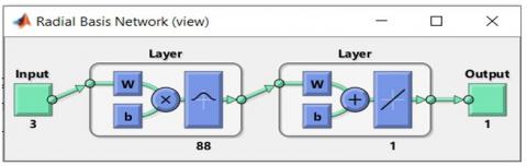
RBF neural networks are feed forward neural networks in structure same as MLP network. It has only one hidden layer as shown in Figure 1. This hidden layer forms the feature vector. A non-linear transfer function called radial basis is applied to the feature vector to increase dimension before being fed for classification.As shown in Figure 1, nodes of hidden layer do radial basis transformation. Here hidden layer outputs are linearly combined with hidden layer outputs to generate final output value. The neural activation function for RBFNN is given by Eq. (4):
$\varphi(x)=e^{-\beta\left\|x-c_i\right\|^2}$ (4)
where, $\beta=\frac{1}{2 \sigma_j^2}$.
Figure 1. Structure of radial basis function neural network
where, $\|.\|$ is the Euclidean norm, c denotes center and σ is a width parameter. The output of a node k of the output layer is given by Eq. (5):
$y_k=\sum_{j=1}^n w_{j k} \varphi_j(x)$ (5)
where normally, Least Mean Square (LMS) algorithm is employed for error minimization by continuous updating weights. Network training is terminated when error condition meets decision threshold criteria. Testing and validation of network is then done for newly updated weights.
RBF networks have been chosen for this study since they tend to be effective in dealing with dataset where data points tend to cluster around a center point. In spectrum data the occupancy tends to cluster in downlink, uplink and center frequencies. RBF networks tend to generalize better and quickly due to their abilities to focus around local clusters. This is an added advantage which makes them less susceptible to over fitting. In RBF networks initially numbers of radial basis functions are determined with their corresponding centers. In this case clustering algorithm like k-means may be used. The next step is to measure closeness of input data with the established center. This is done using a gaussian activation radial basis function. Here weights are determined using least square estimation or gradient descent. Training includes optimization of centers, widths of radial basis functions and weights.
2.2.2 LSTM neural network
LSTM based on Recurrent Neural Network (RNN) architecture deals excellently with data which is temporally correlated; it cannot handle long term time dependency in practice. Basic LSTM cell unit comprises of three gates namely input (i), output (o) and forget (f). These gates have control over what is being read, written and stored in the cell unit. Additionally candidate cell unit (g) is used to add information to cell. An LSTM layer has an output state (called hidden state) and intermediate cell state. LSTM cell unit shown in Figure 2 retains information from past states. At every time step LSTM layer adds or deletes information using gates. In this way long-term dependencies amongst different time steps are learned for time series or sequence data.
Different weights involved in learning include W (Input Weights), R (Recurrent Weights) and b (Bias).
$\boldsymbol{W}=\begin{gathered}W_i \\ W_f \\ W_g\end{gathered}, \, \boldsymbol{R}=\begin{gathered}R_i \\ R_f \\ R_g\end{gathered}, \,\boldsymbol{b}=\begin{gathered}b_i \\ b_f \\ b_g\end{gathered}$,
For every time step t cell state is given by Eq. (6):
$c_t=f_t \odot c_{t-1}+i_t \odot g_t$ (6)
where, ⊙ being the Hadamard product.
For time step t the hidden state is given by Eq. (7):
$\mathrm{h}_{\mathrm{t}}=\mathrm{O}_{\mathrm{t}} \odot \sigma_{\mathrm{c}}\left(\mathrm{c}_{\mathrm{t}}\right)$ (7)
where, σc is the state activation function normally hyperbolic tangent function (tanh).
The formulae’s used for computation at different gates are shown in Table 1.
Figure 2. LSTM cell unit
Table 1. Mathematical formulae for computation at gates
|
Component |
Formula |
|
Input gate |
it=σg(Wi xt+Ri ht −1+bi) |
|
Forget gate |
ft=σg(Wf xt+Rf ht−1+bf) |
|
Cell candidate |
gt=σc(Wg xt+Rght−1+bg) |
|
Output gate |
ot=σg(Woxt+Roht−1+bo) |
where, σg is gate activation function normally sigmoid function $\varphi(x)=\frac{1}{1+e^{-x}}$.
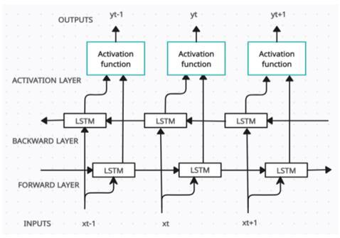
2.2.3 BiLSTM neural network
Individual ANNs like MLP and RBF are prone to vanishing gradient problems when subjected to long sequential data. They are inefficient to capture long term dependencies. To overcome this LSTM/BiLSTM networks are particularly designed to learn from long sequence data. They have memory cell gate units to remember long term dependencies and forget gate mechanism to discard redundant information. This mechanism of selectively remembering and discarding information makes these networks efficient for long datasets like spectrum data. MLP and RBF are suitable for dataset where data points are independent of each other but in case of spectrum dataset where data is sequential a recurrent neural network like LSTM and BiLSTM can offer better results. With this intuition these deep neural networks have been investigated for their performance for spectrum dataset.
Figure 3. BiLSTM network
Better training can beachievedin Bidirectional LSTM (BiLSTM) model by two way information flow one from past and another from future. The immediate advantage of such capability is additional training to enhance prediction accuracy. In Figure 3, a model structure for BiLSTM is shown with different layers and Input/Output.
2.3 Methodology
2.3.1 Proposed methodology
ANNs excel in extracting spatial features of data whereas RNN work very well for temporal dependencies. A hybrid approach thus tends to learn more information and has a better representation. ANNs can generalize data patterns effectively and RNNs can extract contextual information in long sequential data. The spectrum dataset has short term dependencies given by channel vacancy durations and have long term dependencies across locations, services given by service congestion rates [17]. In this work the hybridization of ANN and RNN is being motivated by intrinsic characteristics of data dependencies in spectrum dataset both short term and long term. Our research questions are aimed at determining whether it is possible to produce hybrid models that outperform single models with different domains and types of datasets.
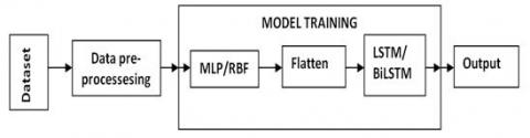
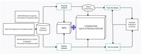
LSTM and BiLSTM are proven algorithms in many applications domains. Here we investigate use of a hybrid model based on these networks for spectrum occupancy inference. We have investigated deep integration of two major recurrent neural networks namely LSTM and BiLSTM to build a hybrid model with RBF. In our proposed model Hybrid RBF-BiLSTM (Hyb R-BiLSTM) has been further analyzed to investigate its competitiveness with existing classical neural networks MLP, RBF, HNN and deep neural networks LSTM, BiLSTM, Hybrid MLP-LSTM (Hyb M-LSTM) and Hybrid MLP-BiLSTM (Hyb M-BiLSTM). The proposed methodology is as illustrated in Figure 4.
Figure 4. Methodology of the proposed Hybrid model
Figure 5. Hybrid R-BiLSTM based spectrum occupancy prediction model architecture
In order to hybridize two different neural network architectures we use a Flatten mechanism to convert the MLP/RBF output to a single featured vector data to be processed by fully connected layer of LSTM/BiLSTM. This mechanism basically reshapes the data vectors to match the mini batch dimensions of underlying layers. The evaluation metrices under consideration includes F1 score, RMSE (Root Mean Square Error), Recall and Precision. This proposed Hybrid R-BiLSTM based spectrum occupancy prediction model architecture is as seen in Figure 5.
The detail steps for predicting future spectrum occupancy states in time and frequency dimensions are outlined in the proposed algorithms. In the first algorithm we train our model with RBFNN model as the first step and then combine the result in second algorithm with Hybrid BiLSTM based prediction.
2.3.2 Proposed algorithms
Algorithm 1: To design a radial basis function network for spectrum inference in cognitive radio network
Input: Historical spectrum occupancy data in time and frequency dimensions with feature vectors
Output: RBFN neural network
Load dataset with feature vectors frequency wise
RBFN Simulation steps
Algorithm 2: To design a hybrid RBFN based BiLSTM network for spectrum inference in cognitive radio network
Input: Historical spectrum occupancy data in time and frequency dimensions with feature vectors
Output: Predicted spectrum occupancy states
Start
#Import predesigned RBFN network from Algorithm 1
#Database creation
#Training
#Testing
#Error & Accuracy Performance Analysis
Stop
2.3.3 Performance metrics for evaluation and comparison
Confusion matrix is used here for quantifying accuracy with performance metrics f1-score, precision and recall. To compare error performance following metrics given by Eqs. (8-10) have been computed.
Mean Absolute Error (MAE):
$M A E=\frac{1}{n} \sum_{\text {sum }}|y-\hat{y}|$ (8)
where, y is true output value and $\hat{y}$ is predicted output value.
Mean Square Error (MSE):
$M S E=\frac{1}{n} \sum_{i=1}^n\left(y_i-\widehat{y}_l\right)^2$ (9)
Root Mean Squared Error (RMSE):
$R M S E=\sqrt{\frac{1}{n} \sum_{i=1}^n\left(y_i-\widehat{y}_l\right)^2}$ (10)
3.1 Dataset generation
3.1.1 Measurement locations and set up
Our spectrum measurement setup comprised of a discone antenna (AOR DA5000), Rohde & Schwarz R&S FSH3 spectrum analyzer and data processing/analysis machine (laptop/PC). Our dataset comprises of spectrum occupancy information measured as Power Spectral Density (PSD) values in dBm across time (ranging from 24 hours to 7 days) and frequency dimensions (0.7 GHz to 2.7 GHz/200KHz resolution) measured across three geographically varying locations (Pune, Solapur, Kalaburagi in India). We intend to cover all telecommunication bands (GSM900, GSM1800, IMT-3G, LTE (2100, 2300)), broadcasting and wireless services, Broadband Wireless Access (BWA), ISM band etc. Out of the entire dataset 70% has been used for training, 20% for testing and 10% for validation of model.
Figure 6. MLP network
3.1.2 Noise thresholding
The noise measurements for threshold calculations were carried out for 2 hours with 50Ω matching load termination. Three popular decision thresholding techniques in literature namely Max Noise, m-dB and PFA noise. After doing competitive analysis of these three techniques PFA thresholding with 1% probability of false alarm setting was selected as threshold viz -91.343dBm, -91.903dBm and -91.616dBm respectively for Pune, Solapur and Kalaburagi.
3.2 ANN based spectrum occupancy prediction
3.2.1 Design of MLP, RBFNN and HNN neural networks
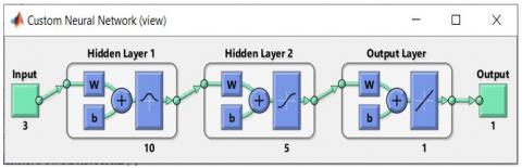
Initially we have used artificial neural networks namely MLP, RBF and HNN (Hybrid Neural Network) for spectrum occupancy prediction [19]. The designed neural networks have been depicted in Figures 6, 7 and 8.
Figure 7. RBF network
Figure 8. Hybrid neural network
The model parameters under considered for spectrum prediction as shown in Table 2.
Table 2. Simulation parameters
|
Parameter |
Value |
|
No. of neurons in first layer |
10 |
|
No. of neurons in the second layer |
05 |
|
No. of hidden layers |
02 |
|
Learning function |
Resilient backpropagation |
|
Learning rate |
0.01 |
|
No. of epochs |
1000 |
|
Achievable goal |
1e-2 |
|
Minimum gradient |
0.000001 |
|
Performance function |
RMSE |
Table 3. Performance comparison of MLP, RBF and HNN neural networks
|
Parameter |
MLP |
RBF |
HNN |
|
No of neurons in first layer |
10 |
88 |
10 |
|
No of neurons in second layer |
5 |
1 |
5 |
|
No of neurons in third layer |
-- |
-- |
1 |
|
No of hidden layers |
2 |
2 |
3 |
|
Accuracy |
75.78% |
100.00% |
84.61% |
Table 4. Confusion matrix for MLP and RBF neural networks
|
|
MLP |
RBF |
HNN |
|||
|
Actual |
Predicted |
Predicted |
Predicted |
Predicted |
||
|
Busy |
Idle |
Busy |
Idle |
Busy |
Idle |
|
|
Busy |
251 (TP) |
84 (FN) |
252 (TP) |
0 (FN) |
252 (TP) |
54 (FN) |
|
Idle |
1 (FP) |
15 (TN) |
0 (FP) |
99 (TN) |
0 (FP) |
45 (TN) |
3.2.2 ANN performance analysis
The error performance comparison of three networks has been summarized in Tables 3 and 4 above. RBF Neural Network shows best performance than MLP and Hybrid Neural Network. The analysis of network performance has been performed by confusion matrix using True positives (TP), True negatives (TN), False Positives (FP) and False Negatives (FN) values
The performance evaluation metrics pecision (π), recall (ψ) and F1- score are defined as follows:
$\pi=\frac{\xi}{\xi+v}, \psi=\frac{\xi}{\xi+\mu}, F_1$ score $=2 \times \frac{\pi \times \psi}{\pi+\psi}$
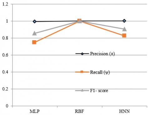
here, ξ (true positive), υ (false positive) and μ (false negative). Major performance metrics precision, recall and F1 score have been computed and listed in Table 5. Thus RBFNN has the best performance with all scores reaching the best values as seen in Figure 9.
Table 5. Performance metrics for ANNs
|
Sr. No |
Parameter |
MLP |
RBF |
HNN |
|
1 |
Precision (π) |
0.996 |
1 |
1 |
|
2 |
Recall (ψ) |
0.7492 |
1 |
0.8253 |
|
3 |
F1- score |
0.8551 |
1 |
0.9043 |
1) Precision (π)=$\frac{T P}{T P+F P}=0.996,1,1$
2) Recall (ψ)=$\frac{T P}{T P+F N}=0.7492,1,0.8253$
3) F1- score=$2 \times \frac{\pi \times \psi}{\pi+\psi}=0.8551,1,0.9043$
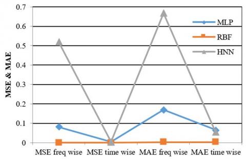
Error Performance graphs in Figures 10-11 and error computations Table 6 clearly depict that RBF Neural Networks outperform MLP and HNN for both time and frequency wise GSM 900 band prediction. These results motivate us to incorporate RBFNN as a hybrid component for proposed Hybrid Deep Neural Network based prediction.
Table 6. Performance metrics for ANNs
|
ANN Technique |
GSM 900 Band (890MHz to 960MHz) |
|||||
|
Frequency Dimension |
Time Dimension |
|||||
|
MSE |
MAE |
RMSE |
MSE |
MAE |
RMSE |
|
|
MLP |
0.0808 |
0.17 |
5.3241 |
0.0047 |
0.0654 |
2.3384 |
|
RBF |
9.56E-06 |
0.0011 |
0.0579 |
9.96E-06 |
0.0019 |
0.1075 |
|
HNN |
0.5201 |
0.6665 |
13.5116 |
0.0033 |
0.0532 |
1.9677 |
Figure 9. Performance comparison of ANN networks
Figure 10. MSE and MAE performance of ANNs
3.3 Hybrid Deep Neural Network based prediction
3.3.1 LSTM and BiLSTM based prediction
Figure 11. RMSE performance of ANNs
Table 7. Simulation parameters
|
Parameter |
Value |
|
No. of features |
03 |
|
No. of Hidden Units |
100 |
|
Response variable |
01 |
|
Optimizer function |
‘adam’ |
|
Learning rate |
0.001 |
|
Maximum epochs |
50 |
|
Performance function |
RMSE |
|
Minimum batch size |
5 |
|
Execution environment |
cpu |
The described data set is now used for training and testing an LSTM and BiLSTM networks. For training and validation of network the model parameters considered for hybrid deep neural network based spectrum prediction are as shown in Table 7.
3.3.2 Spectrum occupancy prediction
Both signal power and band occupancy can be predicted with LSTM/BiLSTM neural network predictor. Figure 12 shows plots of occupancy (duty cycle) being plotted against GSM900 band frequency range 890 MHz to 960 MHz. Here spectrum occupancy plot of the measured data is compared and plotted with the predicted data. The trained model is saved and used for prediction of future signal strengths and occupancy. The predicted signal strengths and occupancy of GSM 900 band at Kondhwa, Pune.
3.3.3 Hybrid R-LSTM and Hybrid R-BiLSTM based prediction
The same data set is now used for training and testing proposed hybrid models Hybrid R-LSTM and Hybrid R-BiLSTM. The results in Figure 13 indicate far more improvement in prediction accuracy. This model combines the advantage of high prediction accuracy of RBFNN after integration with BiLSTM model known for its high prediction accuracy due to forward and backward training capability.
Figure 12. LSTM and BiLSTM GSM900 band occupancy prediction
3.3.4 Network performance analysis
Initially out of total 320 spectrum data points there are 71 Idle (unoccupied) states and 249 Busy (occupied) states for GSM900 band data at Kondhwa Pune location. Using this data confusion matrix in Table 8 is computed for spectrum occupancy data. The sequence length taken into consideration is 31.
Figure 13. Hyb R-LSTM and Hyb R-BiLSTM spectrum occupancy prediction
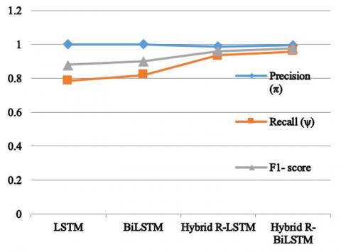
The performance metrics are tabulated in Table 9 and plotted in Figure 14 below.
Figure 14. Performance comparison of hybrid networks
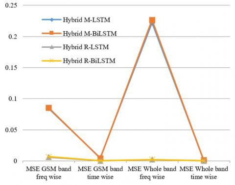
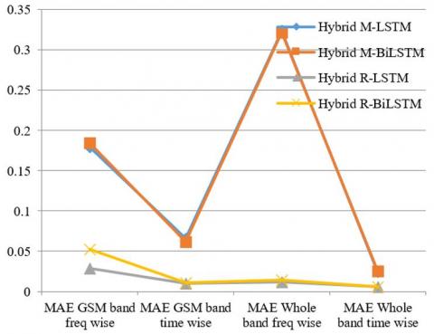
3.3.5 Error performance evaluation and comparison
The error performance comparison of proposed models has been summarized in Table 10. The proposed Hybrid RBF-BiLSTM Neural Network outperforms all other models for both GSM band and Whole band considering time as well as frequency dimension wise predictions. The results have been illustrated graphically in Figures 15-17. Finally the training time in Table 11 and comparison plot Figure 18 depicts improvement in computational speed with the proposed Hyb R-BiLSTM model requiring relatively low training time compared to classical LSTM and BiLSTM with approximately 57% improvement in computation speed.
Table 8. Confusion matrix for LSTM neural networks
|
Channel State/Network |
LSTM |
BiLSTM |
Hybrid R-LSTM |
Hybrid R-BiLSTM |
||||
|
Busy |
Idle |
Busy |
Idle |
Busy |
Idle |
Busy |
Idle |
|
|
Busy |
249 (TP) |
68 (FN) |
249 (TP) |
55 (FN) |
246 (TP) |
17 (FN) |
248 (TP) |
11 (FN) |
|
Idle |
0 (FP) |
3 (TN) |
0 (FP) |
16 (TN) |
3 (FP) |
54 (TN) |
1 (FP) |
60 (TN) |
Table 9. Performance metrics of hybrid networks
|
Sr. No |
Parameter |
LSTM |
BiLSTM |
Hybrid R-LSTM |
Hybrid R-LSTM |
|
1 |
Precision (π) |
1 |
1 |
0.9879 |
0.9959 |
|
2 |
Recall (ψ) |
0.7854 |
0.8190 |
0.9354 |
0.9575 |
|
3 |
F1- score |
0.8798 |
0.9005 |
0.9609 |
0.9763 |
Table 10. Error performance metrics of hybrid networks
|
|
GSM 900 Band (890MHz to 960MHz) |
Whole Band (700MHz to 2.7GHz) |
||||||||||
|
Frequency dimension |
Time dimension |
Frequency dimension |
Time dimension |
|||||||||
|
MSE |
MAE |
RMSE |
MSE |
MAE |
RMSE |
MSE |
MAE |
RMSE |
MSE |
MAE |
RMSE |
|
|
Hybrid M-LSTM |
0.0846 |
0.1792 |
5.2045 |
0.0047 |
0.0657 |
2.2978 |
0.2221 |
0.3238 |
47.6002 |
8.24E-04 |
0.0239 |
1.2354 |
|
Hybrid M-BiLSTM |
0.0855 |
0.1843 |
5.2311 |
0.0041 |
0.0617 |
2.1625 |
0.2264 |
0.3218 |
48.0629 |
9.50E-04 |
0.0252 |
1.327 |
|
Hybrid R-LSTM |
0.0059 |
0.0288 |
1.3686 |
1.60E-04 |
0.0101 |
0.4246 |
2.10E-03 |
0.0117 |
4.6438 |
5.60E-05 |
0.0056 |
0.3221 |
|
Hybrid R-BiLSTM |
0.0067 |
0.0524 |
1.4657 |
1.76E-04 |
0.0107 |
0.4454 |
2.20E-03 |
0.0142 |
4.7177 |
5.48E-05 |
0.0056 |
0.3187 |
Table 11. Performance evaluation of LSTM neural network
|
Technique |
Training Time GSM Band (in seconds) |
Training Time Whole Band (in seconds) |
||
|
Freq dimension |
Time dimension |
Freq dimension |
Time dimension |
|
|
LSTM |
48 |
156 |
3051 |
273 |
|
BiLSTM |
73 |
249 |
6426 |
413 |
|
Hybrid R-LSTM |
47 |
159 |
1783 |
264 |
|
Hybrid R-BiLSTM |
79 |
253 |
2724 |
435 |
Figure 15. MSE comparison plots of hybrid networks
Figure 16. MAE comparison plots of hybrid networks
Figure 17. RMSE comparison plots of hybrid networks
Figure 18. Training time comparison plots of hybrid
In this paper, we have proposed a hybrid deep neural network model combining RBF and BiLSTM neural networks for spectrum inference in cognitive radio network. We tested the performance of this model on our real world spectrum dataset for GSM 900 band (890 MHz to 960 MHz) and entire band (700 MHz to 2.7 GHz) in both time and frequency dimensions.
We compared the performance of this hybrid model with single models like LSTM and BiLSTM. We studied the influence of dataset for both time and frequency dimensions and noted that hybrid model outperforms both single models. We compared performance of hybrid model and single models for precision, recall, F1 score and error performance with metrics MSE, MAE, RMSE. We found that this hybrid approach gives high prediction accuracy and optimal speed.
Our experiments reveal that hybrid approach gives better results for spectrum inference than individual single model approach for spectrum dataset. We have also observed that the effectiveness of this hybrid approach also depends on domain of spectrum dataset.
This hybrid approach can be further enhanced to include spatial dimensions to delve further deep into spectrum dataset. In future this technique can be optimized with a modular approach to fit the requirements of different telecommunication bands. In conclusion hybrid deep neural network can significantly enhance the capabilities of spectrum inference in CRNs.
[1] Mitola, J., Maguire, G.Q. (1999). Cognitive radio: making software radios more personal. IEEE Personal Communications, 6(4): 13-18. https://doi.org/10.1109/98.788210.
[2] Haykin, S. (2005). Cognitive radio: brain-empowered wireless communications. IEEE Journal on Selected Areas in Communications, 23(2): 201-220. https://doi.org/10.1109/JSAC.2004.839380.
[3] Ding, G., Jiao, Y., Wang, J., Zou, Y., Wu, Q., Yao, Y.D., Hanzo, L. (2017). Spectrum inference in cognitive radio networks: Algorithms and applications. IEEE Communications Surveys & Tutorials, 20(1): 150-182. https://doi.org/10.1109/COMST.2017.2751058
[4] Bkassiny, M., Li, Y., Jayaweera, S.K. (2012). A survey on machine-learning techniques in cognitive radios. IEEE Communications Surveys & Tutorials, 15(3): 11361159. https://doi.org/10.1109/SURV.2012.100412.00017.
[5] Arivudainambi, D., Mangairkarasi, S., Varun Kumar, K.A. (2022). Spectrum prediction in cognitive radio network using machine learning techniques. Intell. Autom. Soft Comput, 32(3): 1525-1540.
[6] Eltom, H., Kandeepan, S., Evans, R.J., Liang, Y.C., Ristic, B. (2018). Statistical spectrum occupancy prediction for dynamic spectrum access: A classification. EURASIP Journal on Wireless Communications and Networking, 2018: 1-17. https://doi.org/10.1186/s13638-017-1019-8.
[7] Azmat, F., Chen, Y., Stocks, N. (2015). Analysis of spectrum occupancy using machine learning algorithms. IEEE Transactions on Vehicular Technology, 65(9): 6853-6860. https://doi.org/10.1109/TVT.2015.2487047.
[8] Shrestha, A., Mahmood, A. (2019). Review of deep learning algorithms and architectures. IEEE Access. https://doi.org/10.1109/ACCESS.2019.2912200.
[9] Yu, L., Chen, J., Ding, G. (2017). Spectrum prediction via long short term memory. In 2017 3rd IEEE International Conference on Computer and Communications (ICCC), pp. 643-647. https://doi.org/10.1109/CompComm.2017.8322623
[10] Aygül, M.A., Nazzal, M., Sağlam, M.İ., da Costa, D.B., Ateş, H.F., Arslan, H. (2020). Efficient spectrum occupancy prediction exploiting multidimensional correlations through composite 2D-LSTM models. Sensors, 21(1): 135. https://doi.org/10.3390/s21010135.
[11] Siami-Namini, S., Tavakoli, N., Namin, A.S. (2019). The performance of LSTM and BiLSTM in forecasting time series. In 2019 IEEE International conference on big data (Big Data), pp. 3285-3292. https://doi.org/10.1109/BigData47090.2019.9005997.
[12] Fathi, A.Y., El-Khodary, I.A., Saafan, M. (2023). A hybrid model combining discrete wavelet transform and nonlinear autoregressive neural network for stock price prediction: An application in the Egyptian exchange. Revue d'Intelligence Artificielle, 37(1): 15-21. https://doi.org/10.18280/ria.370103.
[13] Riyaz, L., Butt, M.A., Zaman, M. (2022). A novel ensemble deep learning model for coronary heart disease prediction. Revue d'Intelligence Artificielle, 36(6): 825-832. http://doi.org/10.18280/ria.360602
[14] Kowsher, M., Tahabilder, A., Sanjid, M.Z.I., Prottasha, N.J., Uddin, M.S., Hossain, M.A., Jilani, M.A.K. (2021). LSTM-ANN & BiLSTM-ANN: Hybrid deep learning models for enhanced classification accuracy. Procedia Computer Science, 193: 131-140. https://doi.org/10.1016/j.procs.2021.10.013
[15] Patil, S., Adhiya, K.P. (2023). Evaluation of short answers using domain specific embedding and Siamese stacked BiLSTM with contrastive loss. Revue d'Intelligence Artificielle, 37(3): 719-726. https://doi.org/10.18280/ria.370320.
[16] Wang, X., Chen, Q., Yu, X. (2023). Research on spectrum prediction technology based on B-LTF. Electronics, 12(1): 247. https://doi.org/10.3390/electronics12010247.
[17] Naikwadi, M.H., Patil, K.P. (2022). A multi-dimensional real world spectrum occupancy data measurement and analysis for spectrum inference in cognitive radio network. International Journal of Communication Networks and Information Security, 14(2): 244-260.
[18] Naikwadi, M., Patil, K. (2020). A real time radio spectrum measurement campaign for machine learning based spectrum inference in cognitive radio network. In ICDSMLA 2020: Proceedings of the 2nd International Conference on Data Science, Machine Learning and Applications, pp. 449-457. https://doi.org/10.1007/978-981-16-3690-5_38.
[19] Shirgan, S.S., Bombale, U.L. (2020). Hybrid neural network based wideband spectrum behavior sensing predictor for cognitive radio application. Sensing and Imaging, 21: 1-21. https://doi.org/10.1007/s11220-020-00293-4.